UH-511-1029-03 SLAC-PUB-10000 Dilepton rapidity distribution in the Drell-Yan process at NNLO in QCD

Abstract

We compute the rapidity distribution of the virtual photon produced in the Drell-Yan process through next-to-next-to-leading order in perturbative QCD. We introduce a powerful new method for calculating differential distributions in hard scattering processes. This method is based upon a generalization of the optical theorem; it allows the integration-by-parts technology developed for multi-loop diagrams to be applied to non-inclusive phase-space integrals, and permits a high degree of automation. We apply our results to the analysis of fixed target experiments.

The production of lepton pairs in hadronic collisions, known as the Drell-Yan (DY) process drellyan , was the first application of parton model ideas beyond deep inelastic scattering. Due to its clean theoretical interpretation in terms of quark-antiquark annihilation into a vector boson, and large event rates, the DY process has been studied extensively, and will continue to be investigated at both the Tevatron and the LHC. The DY process provides valuable information about parton distribution functions (pdfs), enables measurements of the production rates and masses of $W$ and $Z$ bosons, and furnishes a sensitive test for many varieties of new physics, such as the additional gauge bosons that appear in many extensions of the Standard Model. It will also be used for the more prosaic purpose of monitoring partonic luminosities at the LHC.

Despite the importance of the DY process and the significant amount of work devoted to its description, the calculation of higher order QCD corrections has proceeded slowly. The next-to-leading order (NLO) QCD corrections to the total cross section, and the $x_{F}$ and rapidity distributions, were calculated nearly 25 years ago alt ; the NNLO corrections to the total cross section were obtained eleven years later Hamberg:1990np . No complete calculation of the NNLO QCD corrections to any differential distribution has been performed, although partial results exist Rijken:1994sh .

Recently, the NNLO virtual corrections to several interesting hard scattering processes in QCD have been computed glover ; however, the calculation of real emission contributions, required for complete NNLO predictions, is still in progress. These contributions entail a careful analysis of perturbative multiparticle final states in generic hard scattering events. While it is certainly useful to solve this problem in complete generality, it is also useful to study specific examples, especially those most urgently needed in experimental analyses. It is possible to develop alternative methods of calculation which can be used to compute basic differential distributions. In Refs. Anastasiou:2002yz ; Anastasiou:2002qz it was shown how to combine the optical theorem with multi-loop computational methods to compute phase space integrals. In this Letter we present a non-trivial application of these ideas; we compute the rapidity distribution of the virtual photon produced in the DY process through NNLO in perturbative QCD.

We shall apply our results to the production of lepton pairs in proton-proton ($pp$) collisions at center-of-mass energies accessible to fixed target experiments. The most recent measurements come from Fermilab experiment E866/NuSea, which measured the dimuon production cross section in $pp$ and proton-deuteron collisions at $\sqrt{s}\approx 40~{}{\rm GeV}$ for muon invariant masses in the interval $4-16~{}{\rm GeV}$ Webb:2003ps . These experiments are sensitive to both the $x\to 1$ components of the valence quark distribution functions and the moderate $x$ components of the sea quark distribution functions of the proton. Neither of these kinematic configurations are well constrained by other data, so the E866 measurements provide valuable input to a global pdf fit. The precision of the E866 measurement is better than 10% per bin. Given the significant ($\sim 40$%) NLO corrections at such energies, the complete NNLO computation is required. Although in principle both photon and $Z$ boson exchanges contribute to this process, the $Z$ exchange component is suppressed by $M^{2}/M_{Z}^{2}$, where $M$ is the invariant mass of the lepton pair. This effect is approximately 1% for the relevant invariant masses, and will be neglected in our analysis.

The NNLO calculation is quite challenging technically. Existing techniques for computing phase-space integrals are incapable of handling problems of this complexity. We introduce here a powerful new method: we extend the optical theorem in such a way that the calculation of differential distributions becomes possible using techniques developed for multi-loop calculations. To achieve this, we represent the rapidity constraint by an effective “propagator.” This propagator is constructed so that when the imaginary part of the forward scattering amplitude is computed using the optical theorem, the “mass-shell” constraint for the “particle” described by this propagator is equivalent to the rapidity constraint in the phase space integration. We then use the methods described in Ref. Anastasiou:2002yz for computing inclusive cross sections, keeping the fake particle propagator in the loop integrals, and deriving the rapidity distribution as the imaginary part of the forward scattering amplitude.

The production of a lepton pair in a high-energy hadronic collision occurs in two distinct steps: first the quarks and gluons from the colliding hadrons annihilate to create a highly virtual time-like photon; then the photon decays into a pair of leptons. In the center-of-mass frame, the two colliding hadrons have momenta $P_{1,2}=\sqrt{s}/2\left(1,{\bf 0}_{\perp},\pm 1\right)$. A virtual photon of invariant mass $M$ produced in the collision has momentum $P_{\gamma}=\left(E,{\bf p}_{\perp},p_{z}\right)$. Its energy and momentum are related by the “mass-shell” condition $E^{2}-{\bf p}_{\perp}^{2}-p_{z}^{2}=M^{2}$, while its rapidity is defined as $\displaystyle Y=\frac{1}{2}\ln\left(\frac{E+p_{z}}{E-p_{z}}\right).$

We first compute the partonic hard scattering cross sections, and then convolute them with the pdfs of the colliding hadrons. The partonic rapidity distributions for the hard scattering of partons $i,j$, with momentum $p_{1}=x_{1}P_{1}$ and $p_{2}=x_{2}P_{2}$ respectively, are obtained by integrating the hard scattering matrix elements over the phase-space of the final state particles with the rapidity and mass of the virtual photon kept fixed:

$$\frac{{\rm d}\sigma_{ij}}{2e^{2Y}{\rm dY}}=\int{\rm d}\Pi_{f}|{\cal M}_{ij}|^{2}\delta\left(e^{2Y}-\frac{E+p_{z}}{E-p_{z}}\right).$$ (1)

The rapidity constraint can be rewritten using the incoming parton momenta as

$$\delta\left(e^{2Y}-\frac{E+p_{z}}{E-p_{z}}\right)=e^{-2Y}\delta\left(\frac{P_{\gamma}\cdot[p_{1}-up_{2}]}{P_{\gamma}\cdot p_{1}}\right),$$ (2)

where $u=\frac{x_{1}}{x_{2}}e^{-2Y}$. The simple Lorentz boost properties of the rapidity are helpful at NNLO. In comparison to the total cross section computation, only one additional dimensionless variable, $u$, is introduced. Computation of the distribution in $x_{F}=2p_{z}/\sqrt{s}$, for example, would require two new variables.

At leading order in $\alpha_{s}$, the production of the virtual photon occurs through the annihilation of a $q\bar{q}$ pair. Only the virtual photon is produced in the collision, rendering the phase-space integrations trivial. At higher orders in $\alpha_{s}$, inelastic channels contribute. At ${\cal O}(\alpha_{s})$, for example, we must consider also $q\bar{q}\to\gamma^{*}g$ and $qg\to q\gamma^{*}$. It is still quite simple to perform these phase space integrations using standard techniques. At higher orders, however, this approach becomes impractical, so we adopt instead the method of Ref. Anastasiou:2002qz , which can be applied efficiently at NNLO.

We first represent the $\delta$-function in Eq. (2) as the imaginary part of an effective propagator:

$$\delta(x)\to\frac{1}{2\pi i}\left[\frac{1}{x-i0}-\frac{1}{x+i0}\right].$$ (3)

Next we map the constrained phase-space integrals onto forward scattering loop integrals Anastasiou:2002yz . We denote the difference of propagators with opposite $i0$ prescription, such as that shown in Eq. (3), by a cut propagator; final state particles on mass-shell are also represented by cut propagators. The $\delta$-function constraint (2) becomes an unconventional propagator, linear in the loop momentum.

At NLO, we must consider integrals of the following general form:

$$I(\nu_{1},\nu_{2},\ldots,\nu_{5})=\int\frac{{\rm d}^{d}k}{(2\pi)^{d}}\frac{1}{A^{\nu_{1}}_{1}\ldots A^{\nu_{5}}_{5}},$$ (4)

where $A_{1}=k^{2}-M^{2}\pm i0,~{}~{}~{}A_{2}=(k+p_{1})^{2},~{}~{}~{}A_{3}=(k+p_{1}+p_{2})^{2}\pm i0,A_{4}=(k+p_{2})^{2}$, and $A_{5}=k\cdot p_{1}-uk\cdot p_{2}\pm i0.$ The propagators $A_{1},A_{3}$ and $A_{5}$ should be “cut” according to Eq. (3), indicating that the corresponding particles are on-shell. The propagators $A_{1..5}$ are linearly dependent; we can therefore eliminate both $A_{2}$ and $A_{4}$ from the integrand in Eq. (4) by partial fractioning. Partial fractioning produces integrals with either $\nu_{1},\nu_{3}$ or $\nu_{5}$ equal to zero. When the cutting rule (3) is applied, such integrals vanish. All phase-space integrals of the form of Eq. (4) can be reduced to a single “master” integral, $I(1,0,1,0,1)$. The fact that only partial fractioning relations are required to perform this reduction is specific to NLO; we will discuss a more general reduction technique when we consider the NNLO corrections.

We compute the virtual corrections to the leading order production process $q\bar{q}\to\gamma^{*}$ in the standard fashion, since the rapidity constraint leaves this calculation unaffected. After combining the real and virtual corrections and performing the collinear factorization, we arrive at the LO and NLO results for the partonic rapidity distributions alt , which we present here for completeness.

We write the partonic differential cross section for the process $i+j\to\gamma^{*}X$, renormalized in the ${\overline{\rm MS}}$ scheme, as

$$(1-z)\frac{{\rm d}\sigma_{ij}}{{\rm dY}}=\eta^{(0)}_{ij}+\left(\frac{\alpha_{s}}{\pi}\right)\eta^{(1)}_{ij}+\left(\frac{\alpha_{s}}{\pi}\right)^{2}\eta^{(2)}_{ij}+{\cal O}(\alpha_{s}^{3}),$$ (5)

where $\alpha_{s}=\alpha_{s}(M)$ is the strong coupling constant assuming $n_{f}$ massless quark flavors, renormalized at the scale $M$. The factorization scale is also set equal to $M$; the dependence on both the renormalization and the factorization scales can be restored by using the renormalization group invariance of the hadronic cross section.

At the lowest order in $\alpha_{s}$, the virtual photon can be produced only in the collision of a quark and antiquark of the same flavor. Therefore,

$$\eta^{(0)}_{ij}=Q_{q}^{2}\left(\delta_{iq}\delta_{\bar{q}j}+\delta_{i\bar{q}}\delta_{qj}\right)\delta(1-z)\left(\delta(y)+\delta(1-y)\right),$$ (6)

where $z=M^{2}/\hat{s}$, $\hat{s}$ is the partonic Mandelstam invariant and $y=(u-z)/(1-z)/(1+u)$.

At NLO, the $q\bar{q}$ channel receives ${\cal O}(\alpha_{s})$ corrections, and the $qg$ and $\bar{q}g$ channels contribute. We find

$$\frac{\eta^{(1)}_{q\bar{q}}}{Q_{q}^{2}}={8\over 3}{z^{2}\over 1+z}\biggl{\{}[\delta(y)+\delta(1-y)]\biggl{[}\delta(1-z)(2\zeta_{2}-4)$$

$$+4\biggl{[}{\ln(1-z)\over 1-z}\biggr{]}_{+}-2(1+z)\ln(1-z)-{1+z^{2}\over 1-z}\ln z$$

$$+1-z\biggr{]}+\biggl{(}1+{(1-z)^{2}\over z}y(1-y)\biggr{)}$$

$$\times\biggl{[}{1+z^{2}\over[1-z]_{+}}\biggl{(}{1\over y_{+}}+{1\over[1-y]_{+}}\biggr{)}-2(1-z)\biggr{]}\biggl{\}},$$ (7)

$$\frac{\eta^{(1)}_{qg}}{Q_{q}^{2}}={z^{2}\over 1+z}\biggl{\{}\delta(y)\biggl{[}[z^{2}+(1-z)^{2}]\ln\frac{(1-z)^{2}}{z}$$

$$+2z(1-z)\biggr{]}+\biggl{(}1+{(1-z)^{2}\over z}y(1-y)\biggr{)}$$

$$\times\biggl{[}[z^{2}+(1-z)^{2}]{1\over y_{+}}+2z(1-z)+(1-z)^{2}y\biggr{]}\biggl{\}}.$$ (8)

Results for the other channels are obtained by permuting partonic labels and changing $y\to 1-y$ in Eqs. (7, 8).

We now discuss the calculation of the NNLO contributions. The purely virtual correction to the rapidity distribution is the same as the virtual correction to the total cross section, and is straightforward to compute using standard techniques. We compute both the real-virtual and the real-real corrections using the method described above. However, to achieve a complete reduction to master integrals at NNLO we must supplement the partial fractioning identities with integration-by-parts (IBP) identities ibps typically used in the reduction of loop integrals. Our substitution of the rapidity constraint with an effective propagator facilitates the use of IBP identities in phase-space integrals. The combined system of equations reduces all required integrals to approximately thirty master integrals, which depend on two variables, $u$ and $z$. The equations are also used to construct differential equations satisfied by the master integrals, following Refs. Anastasiou:2002yz ; Gehrmann:1999as . Here, two first order inhomogeneous partial differential equations are derived for each integral. These equations are solved, and the boundary conditions obtained by considering simple kinematic limits.

At NNLO, the following partonic channels contribute: $q\bar{q}$, the scattering of a quark and anti-quark of the same flavor; $q(\bar{q})g$; $gg$; and $q_{i}q_{j}(\bar{q}_{j})$, the scattering of quarks (anti-quarks) of arbitrary flavor. The complete analytic results for the partonic cross sections are quite lengthy, and will be presented elsewhere.

Integrating the partonic cross sections over the virtual photon rapidity, we reproduce the ${\cal O}(\alpha_{s}^{2})$ correction to the total cross section computed in Ref. Hamberg:1990np . This provides a strong check on our result.

Finally, we must convolute the renormalized partonic cross sections with the partonic structure functions to obtain the experimentally measured cross section. We consider the doubly differential cross section ${\rm d}^{2}\sigma/{\rm d}M{\rm d}Y$:

$$\frac{{\rm d}^{2}\sigma}{{\rm d}M{\rm d}Y}=\frac{4\pi\alpha^{2}}{9M^{3}}\sum_{i,j}\int{\rm d}x_{1}{\rm d}x_{2}f_{i}(x_{1})f_{j}(x_{2})\frac{{\rm d}\sigma_{ij}(z,u)}{{\rm d}Y},$$

where $z=M^{2}/(sx_{1}x_{2})$, $u=(x_{1}/x_{2})e^{-2Y}$, and $\alpha$ is the electromagnetic coupling evaluated at the scale $M$; numerically, $\alpha^{-1}\approx 132$. We use a consistent set of pdfs and $\alpha_{s}$ at each order; the ‘NNLO’ set relies on an approximate set of NNLO splitting kernels martin .

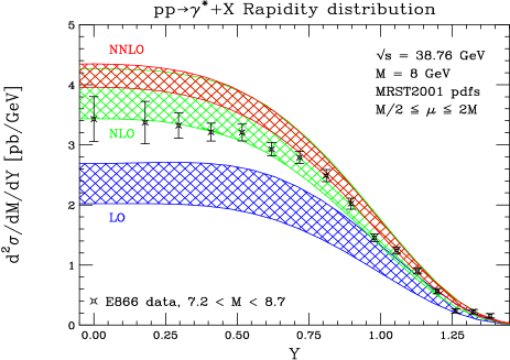
Figure 1: The CMS rapidity distribution of the lepton pair produced in $pp$ collisions at LO (lower band), NLO (middle band), and NNLO (upper band), for parameter choices relevant for fixed target experiments, along with E866 data. The upper (lower) edge of each band denotes the renormalization/factorization scale choice $\mu=M/2$ ($\mu=2M$).

In Fig. 1, we present the center-of-mass system (CMS) rapidity distribution of $M=8$ GeV lepton pairs produced in $pp$ collisions at $\sqrt{s}=38.76$ GeV, along with data from the fixed-target experiment E866/NuSea Webb:2003ps . We set the renormalization and factorization scales both equal to $\mu$. The LO, NLO, and NNLO results are shown as bands in the figure, indicating the variation of the cross sections between the scale choices $\mu=M/2$ and $\mu=2M$. The NLO and NNLO distributions become more sharply peaked at central rapidities; this is due primarily to the evolution of the parton distribution functions beyond leading order. The significant scale dependence of the NLO cross section, which reaches nearly 25% over the interval $M/2\leq\mu\leq 2M$, is reduced to approximately 10% at NNLO. The magnitude of the NNLO corrections depends upon the choice of $\mu$; typically, they increase the NLO result by approximately 5-15%. We note that the NNLO corrections are drastically reduced for the scale choice $\mu=M/2$. The NNLO corrections computed in the so-called “soft” approximation, which retains only those terms that are singular in the limit $z\to 1$, lead to a $\sigma_{\rm NNLO}$ which is lower than the result of the full calculation by approximately $20$% Rijken:1994sh .

The E866 data points are based on measured $x_{F}$ distributions Webb:2003ps , converted from $x_{F}$ to $Y$ with the aid of the $p_{\perp}$ distribution Webb:2003bj . A $\pm 6.5\%$ normalization error common to all data points is not shown. The data lie somewhat below the NNLO prediction at smaller $Y$, and rise to meet it at large $Y$, a trend also visible at other values of $M$. Recall that the antiquark distribution is derived partly from the DY process, fit to the NLO $x_{F}$ distribution. Fitting to our NNLO rapidity distribution instead may result in a smaller antiquark distribution function at moderate $x$. Further comparison with $pd$ as well as $pp$ data is in progress.

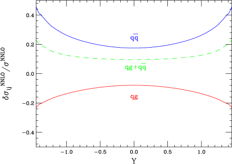
Figure 2: The NNLO corrections for the partonic channels $q\bar{q}$ and $qg$, normalized to the complete NNLO differential cross section, for $\sqrt{s}=38.76$ GeV, $M=8$ GeV, and $\mu=M$.

We now separate our result into its partonic components. The $q\bar{q}$ and $qg$ pieces contribute the majority of the result; the remaining channels are a factor of 50-100 smaller. The magnitude of the NNLO result is determined by a significant cancellation between the $q\bar{q}$ and $qg$ channels. We illustrate this cancellation by plotting the NNLO contributions of these channels, together with their sum, normalized to the complete NNLO differential cross section in Fig. 2. The sum of these channels also contributes a much flatter correction to the rapidity distribution than either piece individually. The $qg$ channel contributes a significant fraction of the complete differential cross section; combining both the NLO and NNLO $qg$ pieces, we find that they account for about 15% of the complete NNLO result for central rapidities, and nearly 40% for larger ($Y\geq 1$) rapidities. This indicates that the NNLO rapidity distribution is quite sensitive to the gluon content of the colliding protons.

Finally, we discuss the dependence of the perturbative K-factors upon rapidity. We define the K-factors as follows: $K^{\rm(N)NLO}(Y)=\sigma^{\rm(N)NLO}/\sigma^{\rm LO}$, and $K^{(2)}(Y)=\sigma^{\rm NNLO}/\sigma^{\rm NLO}$. We present them in Fig. 3. The significant variation of both $K^{\rm NLO}(Y)$ and $K^{\rm NNLO}(Y)$ with rapidity, a nearly 25% change from $Y=0$ to $Y=1$, illustrates that the LO result provides a poor approximation to the shape of the rapidity distribution, as does the LO result weighted by the NNLO K-factor computed from the inclusive cross section. However, the relative flatness of $K^{(2)}$ indicates that the NLO result does accurately predict the shape of the distribution; the NLO differential cross section weighted by $\sigma^{\rm NNLO}/\sigma^{\rm NLO}$, the ratio of NNLO and NLO inclusive cross sections, is valid at these energies to approximately 3-5%. This result appears rather promising, since it suggests a simple and fairly accurate way of incorporating NNLO corrections into NLO Monte Carlo event generators by renormalizing with constant $K$-factors. It remains to be seen, however, if the same conclusion is valid more generally.

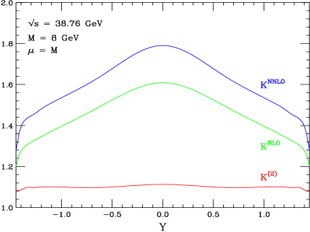
Figure 3: The K-factors $K^{\rm NLO}(Y)=\sigma^{\rm NLO}/\sigma^{\rm LO}$, $K^{\rm NNLO}(Y)=\sigma^{\rm NNLO}/\sigma^{\rm LO}$, and $K^{(2)}(Y)=\sigma^{\rm NNLO}/\sigma^{\rm NLO}$, for $\mu=M$.

In conclusion, we have described a calculation of the NNLO QCD corrections to the rapidity distribution in the Drell-Yan process. We have introduced a powerful new method for the calculation of differential quantities in perturbation theory. Although we have presented only a specific example of this technique, it is clear that this method is of more general applicability; the relation between differential distributions and forward scattering amplitudes described above enables the use of multi-loop technology for the calculation of a large class of phase space integrals. We are confident that this technique will be succesfully applied to compute other quantites of phenomenological interest.

Acknowledgments: This research is partially supported by the DOE under contracts DE-AC03-76SF00515 and DE-FG03-94ER-40833 and by the University of Hawaii startup grant. We thank Mike Leitch and Jason Webb for useful discussions. C. A. thanks the University of Hawaii for kind hospitality during the course of this work.

References

- (1) S.D. Drell and T.M. Yan, Phys. Rev. Lett. 25 (1970), 316.
- (2) G. Altarelli et al., Nucl. Phys. B157, 461 (1979).
- (3) R. Hamberg et al., Nucl. Phys. B 359, 343 (1991) [Erratum-ibid. B 644, 403 (2002)].
- (4) P.J. Rijken and W.L. van Neerven, Phys. Rev.D D51, 44 (1995).
- (5) E.W.N. Glover, hep-ph/0211412, and references therein.
- (6) C. Anastasiou et al., Nucl. Phys. B646, 220 (2002).
- (7) C. Anastasiou et al., arXiv:hep-ph/0211141.
- (8) J.C. Webb et al., arXiv:hep-ex/0302019.
- (9) F.V. Tkachov, Phys. Lett. B100, 65 (1981); K.G. Chetyrkin and F.V. Tkachov, Nucl. Phys. B192, 159 (1981).
- (10) T. Gehrmann and E. Remiddi, Nucl. Phys. B 580, 485 (2000).
- (11) A.D. Martin et al., Phys. Lett. B531 (2002) 216.
- (12) J.C. Webb, arXiv:hep-ex/0301031.