Squark Mixing in Electron-Positron Reactions

Abstract

Squark mixing plays a large role in the phenomenology of the minimal supersymmetric standard model, determining the mass of the lightest Higgs boson and the electroweak interactions of the squarks themselves. We examine how mixing may be investigated in high energy $e^{+}e^{-}$ reactions, both at LEP-II and the proposed linear collider. In particular, off-diagonal production of one lighter and one heavier squark allows one to measure the squark mixing angle, and would allow one to test the mass relations for the light Higgs boson. In some cases off-diagonal production may provide the best prospects to discover supersymmetry. In the context of the light bottom squark scenario, we show that existing data from LEP-II should show definitive evidence for the heavier bottom squark provided that its mass $m_{\tilde{b}_{2}}\leq 120$ GeV.

I Introduction

Scalar quarks, the supersymmetric partners of ordinary colored fermions, are an important ingredient in any theory which combines the standard model (SM) with supersymmetry (SUSY). These scalar partners of the quarks play a key role in the softening of quadratic divergences in the Higgs boson mass parameter induced by loops of quarks. This reduced sensitivity to the ultra-violet physics is the single most attractive feature of the minimal supersymmetric standard model (MSSM). Phenomenologically, scalar quarks (squarks) provide interesting signatures at colliders. They are color triplets, and so may be produced copiously in hadronic reactions. They also couple electroweakly, and thus may have spectacular decays involving leptons and weak bosons. In fact, as quarks in the SM are the fields which ‘bridge’ the strong and electroweak interactions, so squarks are the bridge between the supersymmetric analogues of the gauge sectors. As spin-0 fields, the angular distributions of their production and decay are often quite distinct from their spin-1/2 counterparts.

Each massive quark of the SM results from the marriage (through electroweak symmetry-breaking) of two Weyl fermions with very different electroweak characteristics. Each Dirac fermion is accompanied by two complex scalars, also with distinct electroweak interactions. The supersymmetric versions of the Yukawa interactions between the Higgs boson and the fermions mix this pair of scalars, leading to two mass eigenstates denoted $\tilde{q}_{1}$ and $\tilde{q}_{2}$. The amount of mixing, represented in terms of a mixing angle $\theta_{q}$, is typically proportional to the associated fermion’s mass, and the mixing is thus presumably largest for the third generation squarks.

Squark mixing plays an interesting role in the phenomenology of the MSSM. Perhaps foremost is the fact that the lightest MSSM Higgs boson, the one primarily responsible for electroweak symmetry-breaking, has a mass at tree level which is less than the $Z$ boson mass, considerably smaller than 114.5 GeV, the experimental bound from the CERN Large Electron Positron (LEP) facility lephiggs . This expectation would exclude the MSSM if it were not for the fact that the Higgs boson mass receives large radiative corrections which can lift the mass beyond the reach of the exclusion limits, to masses as large as about 135 GeV. These necessary corrections are provided largely by the top squarks and are enhanced by the squark mixing Carena:1995wu ,

$$m_{H} \simeq M_{Z}^{2}+\frac{3g^{2}m_{t}^{4}}{8\pi^{2}m_{W}^{2}}\left[\log\left(\frac{M_{S}^{2}}{m_{t}^{2}}\right)+x_{t}^{2}\left(1-\frac{x_{t}^{2}}{12}\right)\right].$$ (1)

In this expression, $m_{t}$ is the top quark mass, $M_{S}$ is a common scale of SUSY-breaking which describes the overall magnitude of the squark masses, and $x_{t}=(A_{t}-\mu\cot\beta)/M_{S}$ characterizes the off-diagonal entries in the squark mass matrix (and thus the amount of mixing; $x_{t}\propto\sin\theta_{t}\cos\theta_{t}$), with the largest Higgs boson masses realized for $x_{t}\sim\sqrt{6}$. Once the lightest Higgs boson and top squarks are discovered, a key test that the Higgs boson properties follow the MSSM paradigm will require careful measurement of the top squark masses and their mixing angle. When this dominant correction is understood, one begins to indirectly probe the remainder of the MSSM through the sub-dominant one-loop and dominant two-loop corrections to the Higgs boson mass Heinemeyer:1998jw .

The mixing angle determines the couplings of the squark mass eigenstates to the $W$ and $Z$ bosons. It can be determined efficiently if these couplings are measured. For instance, the rate of the reaction $e^{+}e^{-}\rightarrow\widetilde{q}_{1}^{*}\widetilde{q}_{2}$, production of one lighter and one heavier squark, is proportional to the amount of mixing, and a measurement of the rate is an excellent way to establish the value of the mixing angle. Off-diagonal production provides an interesting complement to other proposals Bartl:2000kw to measure the mixing angle at an electron-positron linear collider lcstudies . These measurements typically involve the cross section for top squark $\tilde{t}_{1}\tilde{t}^{*}_{1}$ pair production with various combinations of polarized $e^{+}$ and $e^{-}$ beams. Off-diagonal production provides an important cross-check of these other methods, and it does not rely on any particular polarization of the incoming beams. Even if the heavier squark mass is larger than half of the collider energy, precluding pair production of the heavier squarks, this method can still succeed and also allow one to measure the mass of the heavier squark.

This line of reasoning is indicative of a general feature of squark phenomenology. While hadron colliders generally offer the best prospects to discover squarks, due to copious production through the strong interactions, it is somewhat problematic to determine parameters in hadronic reactions. In hadron collisions, the primary means to study the electroweak properties of squarks is to examine squark decays. This task is challenging for a number of reasons. In many popular models of SUSY-breaking Abel:2000vs , the squark decay is dominated by a single channel (often into a quark and the lightest neutralino) dictated purely by kinematics, and not by couplings. The branching ratios of various decay modes are relatively insensitive to the squark mixing angle. Furthermore, the squark decay width, the quantity that actually depends on the coupling strength, is in almost all cases well below the experimental resolution and thus unmeasurable at hadron colliders.

This discussion illustrates the importance of squark mixing on the determination of bounds on squark masses from data at lepton colliders. A particular example is furnished by the scenario of light bottom squarks and light gluinos proposed in Ref. Berger:2000mp . In this scenario, the excess rate of bottom quark production at hadron colliders is explained by postulating a tree-level contribution from production of light gluinos which decay into a bottom quark and a bottom squark. Data indicate that the lifetime of the hypothesized light bottom squark must be less than 1 nanosecond Janot:2003cr ; in typical collider detectors, it does not have a significant missing energy signature nor does it produce tracks characteristic of heavy long-lived objects. The light bottom squark $\tilde{b}_{1}$ is assumed to decay hadronically, via R-parity violation, without a visible flavor tag necessarily. Its signals are extremely difficult to extract from backgrounds Berger:2000mp ; Berger:2002kc . Furthermore, a light bottom squark evades LEP-I data if one uses the freedom to select a mixing angle which renders its coupling to the $Z$ boson tiny Carena:2000ka . This essential requirement implies a non-zero mixing angle ($\sin^{2}\theta_{b}\sim 1/6$ ), and, therefore, the off-diagonal $Z$-$\widetilde{b}_{1}$-$\widetilde{b}_{2}$ coupling must be non-zero. Here $\tilde{b}_{2}$ denotes the heavier of two bottom squarks. One of the most promising (and potentially clear) signals of this scenario is furnished by $e^{+}e^{-}\rightarrow Z^{*}\rightarrow\widetilde{b}_{1}\widetilde{b}_{2}$. References to other work on the phenomenology of light bottom squarks and light gluinos may be found in Refs. Berger:2002kc ; Berger:2002vs .

In this article we consider off-diagonal squark production at $e^{+}e^{-}$ colliders. We compute tree-level cross sections and discuss likely decay modes. In Sec. II, we review the squark mass matrix and electroweak interactions. In Sec. III we compute the production cross sections for both bottom squarks and top squarks, showing the dependence on the masses and mixing angles. In Sec. IV we apply our results to the light gluino and bottom squark scenario at LEP-II, estimating for the first time the discovery potential of the heavier bottom squark to be greater than 5 standard deviations ($5\sigma$) provided $m_{\tilde{b}_{2}}\leq 120$ GeV. Alternately, the LEP-II data can exclude masses smaller than 130 GeV, if no signal is observed. We reserve Sec. V for conclusions.

II Squark Masses and Electroweak Interactions

In this section we briefly review the squark mass matrices, mixing angles, and electroweak interactions. The squark mass matrices are

$$\left(\widetilde{t}_{L}^{*}\widetilde{t}_{R}^{*}\right)\left(\begin{array}[]{cc}M_{L}^{2}+m_{t}^{2}+D_{L}&m_{t}(A_{t}-\mu\cot\beta)\\ m_{t}(A_{t}-\mu\cot\beta)&M_{t_{R}}^{2}+m_{t}^{2}+D_{R}\end{array}\right)\left(\begin{array}[]{c}\widetilde{t}_{L}^{*}\\ \widetilde{t}_{R}^{*}\end{array}\right)$$ (6)

for top squarks, and

$$\left(\widetilde{b}_{L}^{*}\widetilde{b}_{R}^{*}\right)\left(\begin{array}[]{cc}M_{L}^{2}+m_{b}^{2}+D_{L}&m_{b}(A_{b}-\mu\tan\beta)\\ m_{b}(A_{b}-\mu\tan\beta)&M_{b_{R}}^{2}+m_{b}^{2}+D_{R}\end{array}\right)\left(\begin{array}[]{c}\widetilde{b}_{L}^{*}\\ \widetilde{b}_{R}^{*}\end{array}\right)$$ (11)

for bottom squarks. Parameters $M_{L}$ and $M_{q_{R}}$ are the SUSY-breaking masses for left- and right-handed squarks, $A_{t}$ and $A_{b}$ are the (SUSY-breaking) trilinear interactions with the Higgs field, $\mu$ is the Higgsino mass parameter, $\tan\beta$ is the ratio of Higgs boson vacuum expectation values (VEVs), $m_{b}$ and $m_{t}$ are the bottom and top quark masses, and and $D_{L}$ and $D_{R}$ are $D$-terms, $D_{L}=m_{Z}^{2}\cos 2\beta(T_{3}-Q_{f}\sin^{2}\theta_{W})$, and $D_{R}=Q_{f}m_{Z}^{2}\sin^{2}\theta_{W}\cos 2\beta$, with $Q_{f}$ the quark charge, and $T_{3}$ its weak isospin. For simplicity, we neglect the possibilities of phases in the soft-breaking parameters; their inclusion is straight-forward.

Diagonalization of the matrices determines the squark mass eigenstates characterized by mixing angles $\theta_{q}$. The physical squarks are a mixture of the scalar partners of the left- and right-chiral quarks. The mass eigenstates are two complex scalars ($\tilde{q}_{1}$ and $\tilde{q}_{2}$), expressed in terms of left-handed (L) and right-handed (R) squarks, $\tilde{q}_{L}$ and $\tilde{q}_{R}$, as

$$|\tilde{q}_{1}\rangle=\sin\theta_{q}|\tilde{q}_{L}\rangle+\cos\theta_{q}|\tilde{q}_{R}\rangle,$$

$$|\tilde{q}_{2}\rangle=\cos\theta_{q}|\tilde{q}_{L}\rangle-\sin\theta_{q}|\tilde{q}_{R}\rangle,$$ (12)

where our convention is that $\widetilde{q}_{1}$ is the lighter of the two mass eigenstates. These angles may be expressed as

$$\sin 2\theta_{t} = \frac{2m_{t}(A_{t}-\mu\cot\beta)}{m_{\tilde{t}_{1}}^{2}-m_{\tilde{t}_{2}}^{2}},$$ (13a)

$$\sin 2\theta_{b} = \frac{2m_{b}(A_{b}-\mu\tan\beta)}{m_{\tilde{b}_{1}}^{2}-m_{\tilde{b}_{2}}^{2}}.$$ (13b)

It is worth emphasizing that the mixing terms in Eq. (11) are proportional to the quark masses, and thus the mixing is presumably largest for the third generation squarks. For this reason, we focus on scalar top and bottom quarks in the discussion below.

The electroweak interactions of the squarks are determined by the relative admixture of left- and right-chiral squark in the mass eigenstate. The coupling to the $SU(2)_{L}$ gauge bosons is only through the left-chiral component, whereas coupling to the $U(1)_{Y}$ boson is non-zero for both. After electroweak symmetry breaking (EWSB), the photon remains massless, and its gauge invariance is linearly realized. All squarks (of a given electric charge) couple equally to the photon with coupling strength given by $Q_{f}e$. The $Z$ boson couplings, on the other hand, are sensitive to the mixing angles,

$$g_{11} = \frac{e}{\sin\theta_{W}\cos\theta_{W}}\left[T_{3}\sin^{2}\theta_{q}-Q_{f}\sin^{2}\theta_{W}\right],$$

$$g_{12} = \frac{e}{\sin\theta_{W}\cos\theta_{W}}\left[T_{3}\sin\theta_{q}\cos\theta_{q}\right],$$

$$g_{22} = \frac{e}{\sin\theta_{W}\cos\theta_{W}}\left[T_{3}\cos^{2}\theta_{q}-Q_{f}\sin^{2}\theta_{W}\right],$$ (14)

where $g_{ij}$ refers to the coupling of the $Z$ boson with $\tilde{q}_{i}$ and $\tilde{q}_{j}$. As mentioned above, the coupling to the lighter squarks may be tuned to vanish for $\sin^{2}\theta_{b}\simeq 1/6$ (for bottom squarks) and $\sin^{2}\theta_{t}\simeq 1/3$ (for top squarks) Carena:2000ka , but in these limits, the off-diagonal couplings, and the heavy-heavy couplings are non-zero.

The couplings to the $W$ boson are

$$g^{W}_{11} = \frac{e}{\sqrt{2}\sin\theta_{W}}\sin\theta_{t}\sin\theta_{b};$$

$$g^{W}_{12} = \frac{e}{\sqrt{2}\sin\theta_{W}}\sin\theta_{t}\cos\theta_{b};$$

$$g^{W}_{21} = \frac{e}{\sqrt{2}\sin\theta_{W}}\cos\theta_{t}\sin\theta_{b};$$

$$g^{W}_{22} = \frac{e}{\sqrt{2}\sin\theta_{W}}\cos\theta_{t}\cos\theta_{b};$$ (15)

where now $g_{ij}$ refers to the coupling of $W$ to $\tilde{t}_{i}$ and $\tilde{b}_{j}$. Squark couplings to quarks and either charginos $\widetilde{\chi}^{\pm}$ or neutralinos $\widetilde{\chi}^{0}$ are straightforward, but somewhat more complicated by the mixing angles associated with the $\widetilde{\chi}^{\pm}$ and $\widetilde{\chi}^{0}$ mass eigenstates.

III Production Cross Sections

In this section, we examine the production of the off-diagonal pair of squarks $\tilde{q}_{1}$ and $\tilde{q}_{2}^{*}$ in the electron-positron annihilation process $e^{+}e^{-}\rightarrow\widetilde{q}_{1}\widetilde{q}^{*}_{2}$, illustrated in Fig. 1. The conjugate process $e^{+}e^{-}\rightarrow\widetilde{q}^{*}_{1}\widetilde{q}_{2}$ has the same cross section. Each reaction has a single Feynman diagram in which a $Z$-boson in exchanged in the $s$-channel. The unbroken gauge invariance of QED forbids the photon from contributing to off-diagonal squark production. For our purposes, it is enough to consider the tree-level production rates. Initial state radiation, and Yukawa and SUSY-QCD one-loop corrections are computed in Ref. Drees:1990te and can be typically as large as $\pm 15\%$ for some regions of parameter space.

III.1 $\bm{e^{+}e^{-}\to}$ $\widetilde{\bm{q}}$₁ $\widetilde{\bm{q}}$$\bm{{}^{*}_{2}}$

Figure 1: Feynman diagram for the process $e^{+}e^{-}\to\tilde{q}_{1}{\tilde{q}}^{*}_{2}$.

The amplitude for the process

$$e^{-}(k_{1})+e^{+}(k_{2})\to Z^{*}\to\tilde{b}_{1}(p_{1},m_{1})+\tilde{b}^{*}_{2}(p_{2},m_{2})$$ (16)

is expressed as

$$\mathcal{M} = g_{12}\bar{v}(k_{2})\gamma_{\mu}(g_{R}P_{R}+g_{L}P_{L})\bar{u}(k_{1})\frac{(p_{1}-p_{2})^{\mu}}{s-M_{Z}^{2}},$$ (17)

where $P_{L}=(1-\gamma_{5})/2$ and $P_{R}=(1+\gamma_{5})/2$. Specified are the four-momenta $k_{1}$ and $k_{2}$ of the incident $e^{-}$ and $e^{+}$, and $p_{1}$ and $p_{2}$ of the final squarks. The lepton couplings to the $Z$ are

$$g_{L} = \frac{e}{\sin\theta_{W}\cos\theta_{W}}\left(-\frac{1}{2}+\sin^{2}\theta_{W}\right);$$ (18a)

$$g_{R} = \frac{e}{\sin\theta_{W}\cos\theta_{W}}\left(\sin^{2}\theta_{W}\right).$$ (18b)

Taking the absolute square of the amplitude, summing over final spins and colors, and averaging over the initial spins, we obtain the differential cross section

$$\frac{d\sigma}{d\cos\theta^{*}} = \frac{r}{32\pi s}\overline{\sum}|\mathcal{M}|^{2}=\frac{3g^{2}_{12}(g_{L}^{2}+g_{R}^{2})}{128\pi s}\frac{r^{3}\sin^{2}\theta^{*}}{\left(1-M_{Z}^{2}/s\right)^{2}},$$ (19)

where

$$r = \frac{2|\mathbf{p}^{*}|}{\sqrt{s}}=\frac{1}{s}\sqrt{(s-m_{1}^{2}-m_{2}^{2})^{2}-4m_{1}^{2}m_{2}^{2}}.$$ (20)

Angle $\theta^{*}$ is the scattering angle of $\tilde{q}_{1}$ in the $e^{+}e^{-}$ center-of-mass frame, and ${\bf p^{*}}$ is its three-momentum. As expected for production of scalar particles, the energy dependence of the cross section is influenced by a $P$-wave threshold factor $\propto|\mathbf{p}^{*}|^{3}$, and the angular distribution varies as $\sin^{2}\theta^{*}$.

The rate integrated over the scattering angle is

$$\sigma = \frac{g^{2}_{12}(g_{L}^{2}+g_{R}^{2})}{32\pi s}\frac{r^{3}}{\left(1-M_{Z}^{2}/s\right)^{2}},$$ (21)

in which the dependence on the squark mixing angle $\theta_{q}$ is manifest in the proportionality to $\sin^{2}2\theta_{q}$ (in the factor of $g_{12}^{2}$) in Eq. (19). For reference, note that production of a $\tilde{q}_{1}$ or a $\tilde{q}_{2}$ pair proceeds through both photon and $Z$ exchange, and is not proportional to $\sin^{2}2\theta_{q}$, containing terms both sensitive and insensitive to the mixing angle.

III.2 Rates at a Linear Collider

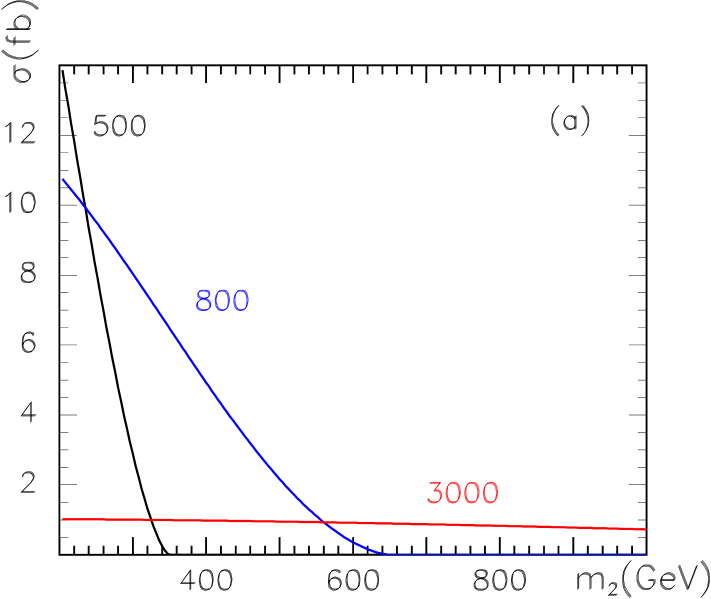
Figure 2: Cross section for the process $e^{+}e^{-}\to\tilde{t}_{1}{\tilde{t}}^{*}_{2}$ at center-of-mass energies 500, 800, and 3000 GeV, as a function of the mass of the heavier top squark and for mixing angle $\sin^{2}\theta_{t}=1/2$. The mass of the lighter top squark has been fixed to 150 GeV.

As discussed above, a key measurement at a future linear collider would be to verify the Higgs boson mass dependence on the supersymmetry-breaking parameters. This test would demonstrate that the MSSM is the effective theory at the weak scale, as opposed to some more general supersymmetric extension. As in most of the MSSM parameter space, the dominant corrections to the Higgs boson mass are from the top squarks, it is their electroweak properties that are most relevant. We envision (for illustrative purposes) a situation in which the Higgs boson has been discovered at the Large Hadron Collider through some combination of production and decay channels (see Ref. atlas:1999fr ), and the squarks have been produced through the strong interaction, dominantly $gg\rightarrow\tilde{t}_{1}^{*}\tilde{t}_{1}$ and $gg\rightarrow\tilde{t}_{2}^{*}\tilde{t}_{2}$. The squark masses and dominant decay channels are likely to be known, but the mixing angle (which plays no role in the tree-level production through the strong force) must be measured at a linear collider.

We consider, for reference, the light top squark to have a mass of 150 GeV, somewhat above the Fermilab Run I bounds Demina:1999ty , although the bounds themselves are sensitive to the details of how the top squark decays. In Fig. 2, we show the cross sections for $e^{+}e^{-}\rightarrow\tilde{t}_{1}^{*}\tilde{t}_{2}$ as a function of the heavier top squark mass, for a reference mixing angle of $\sin^{2}\theta_{t}=1/2$. We choose three center-of-mass energies: $\sqrt{s}=500$, $800$, and $3000$ GeV. The rate is doubled if the charge conjugate process is included. We see that rates are typically of order a few femtobarns (fb) for top squark masses within the range allowed by kinematics. A linear collider with hundreds of inverse fb of data could expect to produce (before cuts) hundreds of events, and the cross section could be measured at the few per cent level, provided experimental efficiencies are not extremely small and backgrounds not prohibitively large. Such questions must be answered in the context of specific top squark decay signatures and are not addressed in this work.

IV Light Bottom Squarks and LEP-II

As our second example, we consider bottom squark production and adopt parameters suggested in the light bottom squark scenario of Ref. Berger:2000mp . This scenario postulates that the excess rate of bottom quark production at hadron colliders arises from pair production of gluinos with masses on the order of 15 GeV. The gluinos subsequently decay to bottom quarks and the light bottom squarks, with masses of order the bottom mass. In order for such light scalar bottom quarks to be consistent with $Z$-pole data, the light bottom squarks must decouple from the $Z$, implying a non-trivial mixing angle $\sin^{2}\theta_{b}\sim 1/6$. Thus, the off-diagonal coupling to the $Z$ boson is necessarily non-zero.

The viability of the light bottom squark scenario has been questioned on the grounds that the heavier $\tilde{b}_{2}$ should have been detected at LEP-II. The argument is based on the evaluation of SUSY-QCD corrections to the $Zb\bar{b}$ vertex in Ref. Cao:2001rz within the context of the light bottom squark and light gluino scenario. These loop corrections contribute negatively to $R_{b}$, the ratio of the width for $Z\rightarrow b\bar{b}$ to the total hadronic width, and they increase in magnitude with the mass of $\tilde{b}_{2}$. To maintain consistency with data, the authors of Ref. Cao:2001rz argue that the mass of $\tilde{b}_{2}$ must be less than 125 (195) GeV at the $2\sigma$ ($3\sigma$) level. In an extension of this analysis, Cho claims that $\tilde{b}_{2}$ must be lighter than $180$ GeV at the $5\sigma$ level Cho:2002mt . A $\tilde{b}_{2}$ in the mass range $<200$ GeV could have been produced in association with a light $\tilde{b}_{1}$ at LEP-II energies, and since no claim of observation has been made, the authors of these studies suggest that LEP data disfavor the light bottom squark scenario. A heavier $\tilde{b}_{2}$ ($\gtrsim 200$ GeV) is allowed if $CP$-violating phases are present Baek:2002xf . Real decays such as $Z\rightarrow\tilde{b}_{1}\bar{b}\tilde{g}+\tilde{b}^{*}_{1}b\tilde{g}$ contribute positively to $R_{b}$ Cheung:2002na and soften these bounds to 160 (290) GeV at the $2\sigma$ ($3\sigma$) level Luo:2003uw . We remark that experimental searches for SUSY particles are model-dependent and a search of LEP-II data for a $\tilde{b}_{2}$ in the light bottom squark scenario has not yet been undertaken. The cross sections and discussion of decay modes in this paper may help to motivate such a search.

We begin with the predicted cross sections and event rates for production of $\tilde{b}_{1}\tilde{b}^{*}_{2}$ pairs at energies explored at the CERN LEP collider. For the large heavy bottom squark masses that we consider, LEP-II is unable to pair-produce heavy bottom squarks, and off-diagonal production is the only viable option. We then discuss decay of $\tilde{b}_{2}$, the heavier of the two bottom squarks. We consider the dominant decay mode $\tilde{b}_{2}\rightarrow b\tilde{g}$, and we evaluate the total width for this decay as a function of $m_{2}$, the mass of $\tilde{b}_{2}$. Subsequently, taking gluino decay into account, we present and evaluate the amplitude for the full three-body decays $\tilde{b}^{*}_{2}\rightarrow b\bar{b}\tilde{b}^{*}_{1}$ and $\tilde{b}^{*}_{2}\rightarrow\bar{b}\bar{b}\tilde{b}_{1}$. The Majorana nature of the gluino permits final states in which there can be bottom quarks of the same sign (i.e., $bb$ or $\bar{b}\bar{b}$) as well as the $b\bar{b}$ configurations expected in SM situations. The overall process, $e^{+}e^{-}\rightarrow\tilde{b}_{1}\tilde{b}^{*}_{2}$, followed by $\tilde{b}_{2}$ decay leads to a four-parton final state.

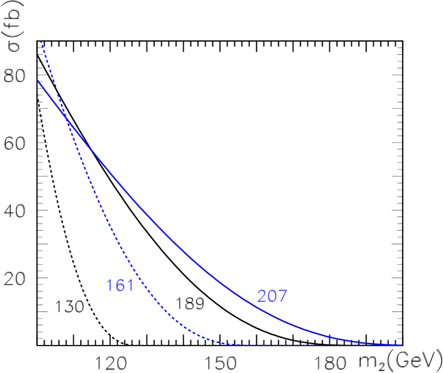
Figure 3: Cross section for the process $e^{+}e^{-}\to\tilde{b}_{1}{\tilde{b}}^{*}_{2}$ at center-of-mass energies 130, 161, 189, and 207 GeV, as a function of the mass $m_{2}$ of the heavier bottom squark. The mass of the lighter bottom squark is $m_{1}=3.5$ GeV, and $\sin^{2}\theta_{b}=1/6$.

IV.1 Cross Sections and Event Rates

Selecting center-of-mass energies spanning those at which data were accumulated at the CERN LEP-II facility, we show the cross section for $\tilde{b}_{1}{\tilde{b}}^{*}_{2}$ production as a function of the mass $m_{2}$ in Fig. 3. In this illustrative calculation, the mass $m_{1}$ of the lighter bottom squark is $m_{1}=3.5$ GeV, and $\sin^{2}\theta_{b}=(2/3)\sin^{2}\theta_{W}\simeq 1/6$. Focusing on the energy dependence at $m_{2}=100$ GeV, we notice that the cross section grows with center-of-mass energy $\sqrt{s}$ from 130 to 161 GeV and then falls as energy increases. This behavior may be traced to the combined influences of the $|\mathbf{p}^{*}|^{3}$ threshold suppression and the usual $1/s$ dependence at large $s$.

Multiplying by the accumulated integrated luminosities per experiment BolekClara at LEP-II, we use our cross sections to compute the predicted number of events produced as a function of $m_{2}$. These results are shown in Fig. 4. Below LEP-II center-of-mass energy 189 GeV, the integrated luminosities were too small to have produced an appreciable sample of events for the process of interest to us. In order to translate the event rates in Fig. 4 into limits on the observability of $\tilde{b}_{2}$, we must discuss likely decay modes, experimental efficiencies, and backgrounds. Decays are discussed in the next subsection. Here we remark simply that if at least 5 events are deemed necessary, the raw event rates in Fig. 4 suggest that a bottom squark with mass greater than 140 GeV will have escaped detection at LEP-II. We present more rigorous estimates below.

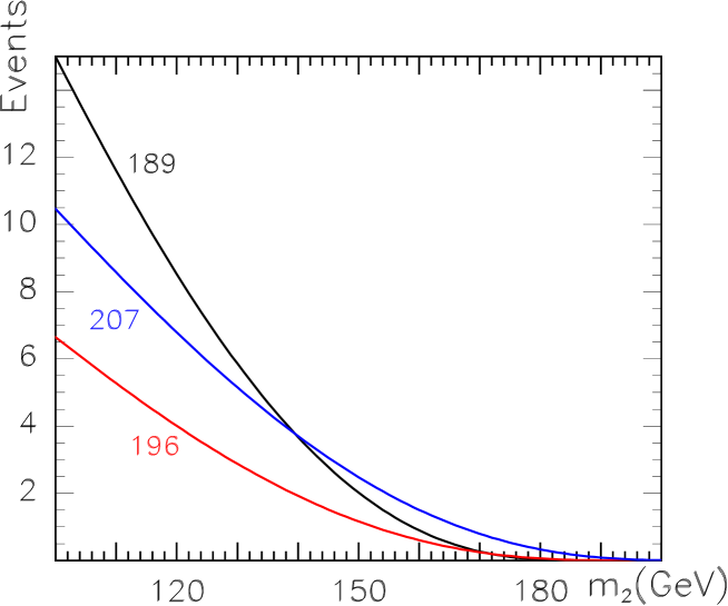
Figure 4: Number of events from $e^{+}e^{-}\to\tilde{b}_{1}{\tilde{b}}^{*}_{2}$ at center-of-mass energies 189, 196, and 207 GeV as a function of the mass $m_{2}$ of the heavier bottom squark. The mass of the lighter bottom squark is $m_{1}=3.5$ GeV, and $\sin^{2}\theta_{b}=1/6$.

IV.2 $\widetilde{b}_{2}$ Decay

In a scenario in which the gluino $\tilde{g}$ is lighter than $\tilde{b}_{2}$, the most likely decay process is $\tilde{b}_{2}\rightarrow b\tilde{g}$. As derived below, both the $\tilde{b}_{2}$ and $\tilde{g}$ widths are narrow compared to their masses, and thus the description of the three-body decay $\tilde{b}_{2}\rightarrow bb\tilde{b}_{1}$ in two sequential steps, $\tilde{b}_{2}\rightarrow\tilde{g}b$ followed by $\tilde{g}\rightarrow b\tilde{b}_{1}$ is an accurate one. The width for $\tilde{b}_{2}\rightarrow\tilde{g}b$, in the $m_{b}=0$ limit, is

$$\Gamma(\tilde{b}_{2}\rightarrow\tilde{g}b) = \frac{2\alpha_{s}(m_{2})}{3}\>m_{2}\>\left(1-\frac{m^{2}_{\tilde{g}}}{m^{2}_{2}}\right)^{2}.$$ (22)

In this expression, $m_{\tilde{g}}$ denotes the gluino mass. In the limit $m_{2}\gg m_{b},m_{\tilde{g}}$, the width grows linearly with $m_{2}$, as expected. To estimate the magnitude of $\Gamma(\tilde{b}_{2}\rightarrow\tilde{g}b)$, we adopt a gluino mass within the range obtained in the light gluino and light bottom squark scenario: $12<m_{\tilde{g}}<16$ GeV. The full width is more than an order of magnitude smaller than the mass $m_{2}$, as expected since the relative size is controlled by $\alpha_{s}(m_{2})\sim 0.1$. For example, choosing $m_{2}=150$ GeV and $m_{\tilde{g}}=15$ GeV, we find $\Gamma_{\tilde{b}_{2}}\simeq 10$ GeV. In our subsequent treatment of the process $e^{+}e^{-}\rightarrow\tilde{b}_{1}\tilde{b}^{*}_{2}$, with $\tilde{b}^{*}_{2}\rightarrow b\bar{b}\tilde{b}^{*}_{1}$ or $\tilde{b}^{*}_{2}\rightarrow\bar{b}\bar{b}\tilde{b}_{1}$, we are justified in adopting the narrow width approximation for $\tilde{b}^{*}_{2}$, factorizing the production and decay.

In the light gluino and light bottom squark scenario, the gluino decays with 100% branching fraction into a bottom quark and and a light bottom squark. However, since the gluino is Majorana in nature, it may decay into either a bottom quark or a bottom anti-quark: $\tilde{g}\rightarrow b\tilde{b}^{*}_{1}$ or $\tilde{g}\rightarrow\bar{b}\tilde{b}_{1}$. As an intermediate step in our full calculation of the width for the three-body decay of $\tilde{b}_{2}$, we first evaluate the width for on-shell gluino decay. The decay width for the two-body subprocess $\tilde{g}\rightarrow b\tilde{b}$ is

$$\Gamma_{\tilde{g}}\equiv\Gamma(\tilde{g}\to b\tilde{b}_{1}^{*})+\Gamma(\tilde{g}\to\bar{b}\tilde{b}_{1}) = \frac{\alpha_{s}(m_{\tilde{g}})}{4}\>m_{\tilde{g}},$$ (23)

where the small bottom and light bottom squark masses are neglected. For $m_{\tilde{g}}=15$ GeV, we find $\Gamma_{\tilde{g}}=0.6$ GeV. We note that corrections to this expression from the finite bottom quark and bottom squark masses are generally not negligible, and introduce a dependence on the squark mixing angle. However, in all cases $\Gamma_{\tilde{g}}\ll m_{\tilde{g}}$, and these corrections have little effect on the heavy bottom squark width or the distributions of the (highly boosted) gluino decay products from $\tilde{b}_{2}$ decays.

Table 1: The decay widths $\Gamma_{\textrm{LS}}$ and $\Gamma_{\textrm{OS}}$ in GeV obtained with $m_{\tilde{g}}$=15 GeV, $\sin^{2}\theta_{b}=1/6$, and $\alpha_{s}(m_{2})=$0.116, 0.112, 0.109 and 0.108 for $m_{2}=$100, 125, and 150, and 175 GeV, respectively. Also shown is the total $\Gamma_{\tilde{b}_{2}}$.

$m_{2}=$	100 GeV	125 GeV	150 GeV	175 GeV
$\Gamma_{\textrm{LS}}$	3.8 GeV	4.6 GeV	5.4 GeV	6.2 GeV
$\Gamma_{\textrm{OS}}$	3.6 GeV	4.5 GeV	5.4 GeV	6.2 GeV
$\Gamma_{\tilde{b}_{2}}$	7.4 GeV	9.1 GeV	10.8 GeV	12.4 GeV

IV.3 $\widetilde{\bm{b}}$$\bm{{}^{*}_{2}}$ $\to$ $b\bar{b}$ $\widetilde{\bm{b}}$$\bm{{}^{*}_{1}}$ and $\widetilde{\bm{b}}$$\bm{{}^{*}_{2}}$ $\to$ $\bar{b}\bar{b}$ $\widetilde{\bm{b}}$₁

Figure 5: Feynman diagram for the decay $\tilde{b}^{*}_{2}\to b\bar{b}\tilde{b}^{*}_{1}$.

Figure 6: Feynman diagrams for the decay $\tilde{b}^{*}_{2}\to\bar{b}\bar{b}\tilde{b}_{1}$.

In this subsection, we address the full three-body decay subprocesses $\tilde{b}^{*}_{2}\to b\bar{b}\tilde{b}^{*}_{1}$ and $\tilde{b}^{*}_{2}\to\bar{b}\bar{b}\tilde{b}_{1}$. The relevant Feynman diagram in the case of opposite sign ‘OS’ production ($b\bar{b}$) is shown in Fig. 5, and the two diagrams for like-sign ‘LS’ production in Fig. 6. For OS and LS decay, our kinematic notation is

OS $$: \tilde{b}_{2}^{*}(s_{2})\to b(p_{1})+\bar{b}(p_{2})+\tilde{b}_{1}^{*}(p_{\tilde{b}});$$ (24a)

LS $$: \tilde{b}_{2}^{*}(s_{2})\to\bar{b}(p_{1})+\bar{b}(p_{2})+\tilde{b}_{1}(p_{\tilde{b}}),$$ (24b)

where the quantities in parenthesis are 4-momenta. In evaluating the amplitudes for these decays, we must contend with the fact that the gluino goes onto its mass-shell within the physical region. To handle this singularity, we resum a class of contributions to the imaginary part of the gluino 2-point function to all orders, replacing the gluino propagator by a Breit-Wigner form, $p^{2}-m^{2}_{\tilde{g}}\rightarrow p^{2}-m_{\tilde{g}}^{2}+im_{\tilde{g}}\Gamma_{\tilde{g}}$, and we use the expressions for $\Gamma_{\tilde{g}}$ above. Explicit expressions for the matrix elements and decay widths are presented in the Appendix.

Defining

$$\Gamma_{\textrm{LS}} = \Gamma(\tilde{b}^{*}_{2}\to\tilde{b}_{1}+\bar{b}\bar{b}),$$ (25a)

$$\Gamma_{\textrm{OS}} = \Gamma(\tilde{b}^{*}_{2}\to\tilde{b}_{1}+b\bar{b}),$$ (25b)

we provide numerical values of these two widths in Table 1 for four interesting values of $m_{2}$, $m_{\tilde{g}}=15$ GeV, and $\sin^{2}\theta_{b}=1/6$. For comparison, we also present the inclusive $\tilde{b}_{2}$ width computed from the two-body decay matrix elements, Eq. (22). It is notable that the LS width is substantial in all cases, and is in fact slightly larger than the OS width for the lighter $\tilde{b}_{2}$ masses we consider. The sum of the LS and OS widths, obtained from the three-body decay amplitudes, equals to good accuracy the inclusive width obtained from the two-body decay process. In general, the decay widths may depend on the sign of the product $\cos\theta_{b}\sin\theta_{b}$, but this dependence is absent in the limit that $m_{b}$ and $m_{1}$ vanish.

Production of like-sign pairs, attributable directly to the Majorana nature of the gluino means that the subprocess of interest here generates apparent “time = zero” $B^{0}-\bar{B}^{0}$ flavor-anti-flavor mixing in $e^{+}e^{-}$ annihilation at LEP-II and linear collider energies. However, the $\tilde{b}_{2}^{*}\tilde{b}_{1}$ production process results in one or two jets in addition to the jets containing the $b$ and $\bar{b}$, and thus these events may not be included in a measurement of $B^{0}-\bar{B}^{0}$ mixing that focuses on $b\bar{b}$ production without additional radiation. The fraction of the decays that lead to like-sign pairs of $b$’s is

$$B_{\textrm{LS}} = \frac{\Gamma_{\textrm{LS}}}{\Gamma_{\textrm{LS}}+\Gamma_{\textrm{OS}}}\approx\frac{\Gamma(\tilde{g}\to\tilde{b}_{1}+\bar{b})}{\Gamma(\tilde{g}\to\tilde{b}_{1}+\bar{b})+\Gamma(\tilde{g}\to\tilde{b}^{*}_{1}+b)},$$ (26)

and from Table 1, we see that this ratio is close to $\frac{1}{2}$ for all of the heavy bottom squark masses of interest, with LS slightly dominant for smaller $\tilde{b}_{2}$ masses.

IV.4 Signatures and Discovery Potential at LEP-II

The overall process, $e^{+}e^{-}\rightarrow\tilde{b}_{1}\tilde{b}^{*}_{2}$, followed by $\tilde{b}_{2}$ decay leads to a four-parton final state. The light bottom squarks carry color and are expected to be observed as hadronic jets. Absent model-dependent assumptions about bottom squark decays, these jets may have no special flavor content. Our SUSY subprocess results therefore in a four-jet final state: with 2 $b$ jets and 2 $\widetilde{b}$ jets.

The massive $\tilde{b}^{*}_{2}$ is produced in $e^{+}e^{-}\to\tilde{b}_{1}\tilde{b}^{*}_{2}$ with relatively little momentum. The three products from its decay will therefore inherit little sense of direction. The distribution in $\cos\theta_{1j}$ will tend to be fairly flat; subscript $1$ denotes the primary $\tilde{b}_{1}$, and $j$ labels one of the decay products of the $\tilde{b}_{2}$. The heavy parent $\tilde{b}^{*}_{2}$ tosses off a $\bar{b}$ and a gluino, both with substantial but oppositely directed momentum. The gluino then decays into a $\tilde{b}_{1}$ and the second $b$ or $\bar{b}$, with the daughter particles retaining the direction of the gluino’s momentum. Since the daughter $b$ or $\bar{b}$ follows the direction of the gluino, the two final $b$’s, in the event, whether like-sign or opposite-sign, emerge in opposite hemispheres in the overall $e^{+}e^{-}$ system. The invariant mass of the two final $b$’s will tend to be large. Furthermore, since $m_{\tilde{g}}\ll m_{2}$, we expect the $\tilde{g}$ to be highly boosted, with a small opening angle between its decay products.

The two $b$ jets are predicted to emerge in a fairly back-to-back configuration, much as is expected from a standard model QCD subprocess $e^{+}e^{-}\rightarrow(\gamma,Z^{*})\rightarrow b\bar{b}g$, with $g\rightarrow$ one or more ${\rm jet}$s. (One of the $\tilde{b}$ jets may emerge fairly close to one of the $b$ jets, resulting in a three-jet topology, as we investigate below.) The configuration produced by the SUSY process differs from that associated with $e^{+}e^{-}\rightarrow(\gamma,Z^{*})\rightarrow q\bar{q}g$ with $g\rightarrow b\bar{b}$. In this later process, gluon splitting would yield $b\bar{b}$ pairs with modest invariant mass.

The key question is how heavy the second scalar bottom quark $\tilde{b}_{2}$ might be and still be discovered lurking in the LEP-II data. Alternately, one can ask what range of heavy bottom squark masses are ruled out by the data, if no signal is observed. We concentrate on the high luminosity run at $\sqrt{s}=207$ GeV at LEP-II, as it provides the greatest number of events for the masses of interest (c.f. Fig. 4). For this analysis, we do not distinguish the LS $\bar{b}\bar{b}$ and OS $b\bar{b}$ situations, adding the distributions generated in the two cases. There would likely be greater potential for identifying the SUSY events if there were experimental capability to separate $b$ and $\bar{b}$ jets.

To answer our question, we address first the experimental signature of the off-diagonal bottom squark production process. The two bottom quark jets are almost always distinguishable, with a large separation between them. Similarly, the “primary” light bottom squark tends to be visible as a distinct jet of hadrons. However, the light bottom squark from the $\tilde{g}$ decay is often rather collinear with the bottom quark from the same decay, because the $\tilde{g}$ tends to be boosted by the heavy bottom squark mass. Thus, we must establish the number of distinctly observable jets in the final state.

We define an observable jet as one with transverse momentum ($p_{T}$) greater than 10 GeV, lying in the central region of the detector, $|y|\leq 2$, where $y$ is the jet rapidity. The separation between two jets is quantified by $\Delta R\equiv\sqrt{\Delta y^{2}+\Delta\phi^{2}}$, where $\Delta\phi$ is the difference in azimuthal angles. We consider two jets distinct from one another provided $\Delta R\geq 0.4$; for smaller $\Delta R$ they are merged into a single jet. The distribution in the number of jets depends on the $\tilde{b}_{2}$ mass. For $m_{2}\sim 120$ GeV, we find that the rate is split roughly evenly between $3$ jets and $4$ jets. For a heavier $m_{2}\sim 150$ GeV, the rate is split roughly as $2/3$ $3$-jet events and $1/3$ $4$-jet events. The difference arises because the larger $\tilde{b}_{2}$ mass results in a more highly boosted gluino, and thus more collinear decay products which are more likely to be merged into a single jet. For both masses, the $2$-jet rates are smaller than a few per cent of the inclusive cross sections. We focus on detection of the $4$-jet channel because its rate is a large fraction of the total rate for all masses of interest, and because we expect that the $4$-jet configuration has smaller backgrounds,

Backgrounds arise from $e^{+}e^{-}\rightarrow 3$ jets and $4$ jets, respectively, and involve a variety of mixed QCD-electroweak and purely weak processes. We simulate the $4$-jet background using matrix elements from MADGRAPH Murayama:1992gi . After the acceptance cuts described above, we find backgrounds are typically much larger than the signal rates, hundreds of fb compared to 30 fb (6 fb) for $m_{2}=120$ GeV (150 GeV). These may be reduced by positing a mass for the heavy bottom squark, and demanding that three of the jets reconstruct this mass within some window. Since the width of the heavy bottom squark is generally of order 10 GeV in the mass range of interest, we consider an invariant mass cut such that any three of the jets reconstruct an invariant mass within 10 GeV of $m_{2}$. This $m_{2}$-dependent cut thus forces the background to vary with the hypothesized value of $m_{2}$. After its application, we find that the background is reduced to the manageable levels of 20 fb (43 fb) at 120 GeV (150 GeV).

For both masses, the number of combined signal and background events is $\geq 8$, and thus one may apply Gaussian statistics to determine the statistical significance in the usual way, with $\sigma\equiv S/\sqrt{S+B}$ providing the confidence level (CL) for an observed signal, with $S$ signal events and $B$ background events. The resulting significances are about $5\sigma$ ($0.4\sigma$) at $m_{2}=120$ GeV (150 GeV). Thus, LEP-II should be able to discover the heavier bottom squark through off-diagonal production if its mass is less 120 GeV. If no signal is observed, we estimate that masses less than 130 GeV can be excluded at the $95\%$ CL. Our analysis could be improved in a number of ways, notably if experimental acceptances and efficiencies were incorporated, a task beyond the scope of this work. It is our hope that the analysis in this paper and the exciting prospect of the discovery of SUSY will motivate a detailed search for signals in existing LEP-II data.

V Conclusions

Mixing between weak doublets and singlets is a novel feature of the scalar fermion sector of the MSSM. Aside from leading to interesting phenomenology, this mixing (in the top squark sector) is also important, allowing for large radiative corrections to the mass of the lightest Higgs boson, needed if the MSSM is to survive the challenge of the negative Higgs boson searches at LEP-II. Turning this statement around, once scalar tops are observed, and their masses and mixing determined, one can, to a fair degree of accuracy, determine whether the theory at the TeV scale is described by the MSSM, or by some more exotic extension.

In this article we explore the off-diagonal squark production mode at $e^{+}e^{-}$ colliders as a means to measure the mixing angle and to learn more about the MSSM itself. Squark mixing arises from a combination of supersymmetric interactions and SUSY-breaking masses and trilinear terms. These in turn are related closely to the flavor structure of the MSSM. While there are many reasons to prefer the MSSM as the theory of physics beyond the standard model, its intense flavor problem indicates that SUSY-breaking is somehow very special such that flavor violation has not yet been observed in low energy experiments. Measurements of the flavor-full soft parameters will be the first experimental indications as to how nature has chosen to solve the SUSY flavor problem, and thus how SUSY is broken and the breaking communicated to the MSSM fields.

Squark mixing is also a key player in defining the properties of the squarks themselves, determining the coupling to the massive electroweak bosons. Light bottom squarks, an interesting ingredient in the supersymmetric resolution of the bottom quark production cross section at hadron colliders Berger:2000mp , escape detection at LEP-I because their mixing angle is such that the left-handed and right-handed interactions with the $Z$ boson cancel each other. This feature necessarily implies that off-diagonal production is non-zero and can be used to discover or constrain the mass of the heavier bottom squark. With a careful, dedicated analysis of existing LEP-II data, we show in this paper that it should be possible to discover heavy bottom squarks at the $5\sigma$ level with masses as large as 120 GeV. If no signal is observed, exclusion limits at the $95\%$ CL should be feasible for masses of the order of 130 GeV and less. Off-diagonal squark production thus allows one to explore a large portion of the parameter space of the light bottom squark scenario.

Appendix

In this Appendix, we present the matrix elements for the full three-body decay subprocesses $\tilde{b}^{*}_{2}\to b\bar{b}\tilde{b}^{*}_{1}$ and $\tilde{b}^{*}_{2}\to\bar{b}\bar{b}\tilde{b}_{1}$, keeping the dependence on the two large masses: $m_{2}$ and $m_{\tilde{g}}$. The relevant Feynman diagram in the case of opposite sign ‘OS’ production ($b\bar{b}$) is shown in Fig. 5 and the two diagrams for like-sign ‘LS’ production in Fig. 6. The 4-momenta are labeled as $p_{1}$ and $p_{2}$ for the two bottom quarks; in the case of OS production, $p_{1}$ refers to the $b$ and $p_{2}$ to the $\bar{b}$. The 4-momentum of the light bottom squark is denoted $p_{\tilde{b}}$. In the LS case, we include in $\overline{|\mathcal{M}|^{2}}$ the symmetry factor $\frac{1}{2}$ for identical particles in the final state.

The explicit expressions for these invariant amplitudes, summed/averaged over final/initial colors and spins are:

$$\overline{|\mathcal{M}|^{2}_{\textrm{LS}}} = \frac{4g_{S}^{4}}{3}\bigg{\{}\left[2\left(1+\cos^{2}2\theta_{b}\right)(p_{1}\cdot p_{\tilde{b}})(p_{2}\cdot p_{\tilde{b}})+m_{\tilde{g}}^{2}\left(1-\cos^{2}2\theta_{b}\right)(p_{1}\cdot p_{2})\right]\left[|c_{1}|^{2}+|c_{2}|^{2}\right]$$ (27a)

$$-\frac{2\sin^{2}2\theta_{b}}{3}\left[m_{\tilde{g}}^{2}(p_{1}\cdot p_{2})+2(p_{1}\cdot p_{\tilde{b}})(p_{2}\cdot p_{\tilde{b}})\right]{\rm Re}\>\left(c_{1}c_{2}^{*}\right)\bigg{\}}$$

$$\overline{|\mathcal{M}|^{2}_{\textrm{OS}}} = \frac{8g_{S}^{4}}{3}|c_{1}|^{2}\left\{\left(1+\cos^{2}2\theta_{b}\right)m_{\tilde{g}}^{2}(p_{1}\cdot p_{2})+2\left(1-\cos^{2}2\theta_{b}\right)(p_{1}\cdot p_{\tilde{b}})(p_{2}\cdot p_{\tilde{b}})\right\}$$ (27b)

with

$$c_{i} = \frac{1}{((p_{i}+p_{\tilde{b}})^{2}-m_{\tilde{g}}^{2})^{2}+m_{\tilde{g}}^{2}\Gamma_{\tilde{g}}^{2}}\>,$$ (28a)

$$\textrm{Re}[c_{1}c^{*}_{2}] = \frac{((p_{1}+p_{\tilde{b}})^{2}-m_{\tilde{g}}^{2})((p_{2}+p_{\tilde{b}})^{2}-m_{\tilde{g}}^{2})+m_{\tilde{g}}^{2}\Gamma_{\tilde{g}}^{2}}{\left[((p_{1}+p_{\tilde{b}})^{2}-m_{\tilde{g}}^{2})^{2}+m_{\tilde{g}}^{2}\Gamma_{\tilde{g}}^{2}\right]\left[((p_{2}+p_{\tilde{b}})^{2}-m_{\tilde{g}}^{2})^{2}+m_{\tilde{g}}^{2}\Gamma_{\tilde{g}}^{2}\right]}\>.$$ (28b)

To obtain the partial widths we integrate these expressions over the three body phase space for the 3 approximately massless final state particles. The resulting partial widths are shown in Table 1.

References

- (1) LEP Higgs Working Group for Higgs Boson Searches, Proceedings of the International Europhysics Conference on High Energy Physics (HEP 2001), Budapest, Hungary, July 12-18, 2001, arXiv:hep-ex/0107029 and arXiv:hep-ex/0107030.
- (2) M. Carena, M. Quiros, and C. E. M. Wagner, Nucl. Phys. B 461, 407 (1996) [arXiv:hep-ph/9508343]; H. E. Haber, R. Hempfling, and A. H. Hoang, Z. Phys. C 75, 539 (1997) [arXiv:hep-ph/9609331].
- (3) S. Heinemeyer, W. Hollik, and G. Weiglein, Phys. Rev. D 58, 091701 (1998) [arXiv:hep-ph/9803277]; S. Heinemeyer, W. Hollik, and G. Weiglein, Phys. Lett. B 440, 296 (1998) [arXiv:hep-ph/9807423]; S. Heinemeyer, W. Hollik, and G. Weiglein, Eur. Phys. J. C 9, 343 (1999) [arXiv:hep-ph/9812472]; J. R. Espinosa and R. J. Zhang, J. High Energy Phys. 0003, 026 (2000) [arXiv:hep-ph/9912236]; J. R. Espinosa and R. J. Zhang, Nucl. Phys. B 586, 3 (2000) [arXiv:hep-ph/0003246]; M. Carena, H. E. Haber, S. Heinemeyer, W. Hollik, C. E. M. Wagner, and G. Weiglein, Nucl. Phys. B 580, 29 (2000) [arXiv:hep-ph/0001002]; G. Degrassi, P. Slavich, and F. Zwirner, Nucl. Phys. B 611, 403 (2001) [arXiv:hep-ph/0105096]; A. Brignole, G. Degrassi, P. Slavich, and F. Zwirner, arXiv:hep-ph/0112177.
- (4) A. Bartl, H. Eberl, S. Kraml, W. Majerotto, and W. Porod, Eur. Phys. J. C 2, 6 (2000) [arXiv:hep-ph/0002115]; A. Finch, H. Nowak, and A. Sopczak, arXiv:hep-ph/0211140.
- (5) American Linear Collider Working Group, T. Abe et al, “Linear Collider Physics Resource Book for Snowmass 2001”, SLAC-R-570; TESLA Technical Design Report, Ed. by R. Heuer, D. Miller, F. Richard, A. Wagner, and P. Zerwas, www.desy.de/ lcnotes/tdr.
- (6) For some well-motivated examples, see S. Abel et al. [SUGRA Working Group Collaboration], arXiv:hep-ph/0003154; R. Culbertson et al. [SUSY Working Group Collaboration], arXiv:hep-ph/0008070; L. Randall and R. Sundrum, Nucl. Phys. B 557, 79 (1999) [arXiv:hep-th/9810155]; G. F. Giudice, M. A. Luty, H. Murayama, and R. Rattazzi, JHEP 9812, 027 (1998) [arXiv:hep-ph/9810442]; D. E. Kaplan, G. D. Kribs, and M. Schmaltz, Phys. Rev. D 62, 035010 (2000) [arXiv:hep-ph/9911293]; Z. Chacko, M. A. Luty, A. E. Nelson, and E. Ponton, JHEP 0001, 003 (2000) [arXiv:hep-ph/9911323]; M. Schmaltz and W. Skiba, Phys. Rev. D 62, 095005 (2000) [arXiv:hep-ph/0001172]; D. E. Kaplan and T. M. P. Tait, JHEP 0006, 020 (2000) [arXiv:hep-ph/0004200].
- (7) E. L. Berger, B. W. Harris, D. E. Kaplan, Z. Sullivan, T. M. P. Tait, and C. E. M. Wagner, Phys. Rev. Lett. 86, 4231 (2001) [arXiv:hep-ph/0012001].
- (8) P. Janot, CERN-EP/2003-004, arXiv:hep-ph/0302076, to be published in Phys. Lett. B; ALEPH Collaboration, A. Heister et al, CERN-EP/2003-024, submitted to the Eur. Phys. Jour. C.
- (9) E. L. Berger, Int. J. Mod. Phys. A 18, 1263 (2003) [arXiv:hep-ph/0201229]; E. L. Berger, arXiv:hep-ph/0209374.
- (10) M. Carena, S. Heinemeyer, C. E. M. Wagner, and G. Weiglein, Phys. Rev. Lett. 86, 4463 (2001) [arXiv:hep-ph/0008023].
- (11) E. L. Berger, C. W. Chiang, J. Jiang, T. M. P. Tait, and C. E. M. Wagner, Phys. Rev. D 66, 095001 (2002) [arXiv:hep-ph/0205342].
- (12) M. Drees and K. I. Hikasa, Phys. Lett. B 252, 127 (1990); W. Beenakker, R. Hopker, and P. M. Zerwas, Phys. Lett. B 349, 463 (1995) [arXiv:hep-ph/9501292]; K. I. Hikasa and J. Hisano, Phys. Rev. D 54, 1908 (1996) [arXiv:hep-ph/9603203]; H. Eberl, A. Bartl, and W. Majerotto, Nucl. Phys. B 472, 481 (1996) [arXiv:hep-ph/9603206]; H. Eberl, S. Kraml, and W. Majerotto, JHEP 9905, 016 (1999) [arXiv:hep-ph/9903413].
- (13) M. Carena et al., “Report of the Tevatron Higgs working group,” arXiv:hep-ph/0010338; ATLAS Collaboration, “ATLAS detector and physics performance. Technical design report, Vol. 2, CERN/LHCC/99-15 (1999); CMS Collaboration, Technical Proposal, report CERN/LHCC/94-38 (1994).
- (14) R. Demina, J. D. Lykken, K. T. Matchev, and A. Nomerotski, Phys. Rev. D 62, 035011 (2000) [arXiv:hep-ph/9910275]; E. L. Berger, B. W. Harris, and Z. Sullivan, Phys. Rev. D 63, 115001 (2001) [arXiv:hep-ph/0012184].
- (15) J. J. Cao, Z. H. Xiong, and J. M. Yang, Phys. Rev. Lett. 88, 111802 (2002) [arXiv:hep-ph/0111144].
- (16) G. C. Cho, Phys. Rev. Lett. 89, 091801 (2002) [arXiv:hep-ph/0204348].
- (17) S. Baek, Phys. Lett. B 541, 161 (2002) [arXiv:hep-ph/0205013].
- (18) K. Cheung and W. Y. Keung, Phys. Rev. D 67, 015005 (2003) [arXiv:hep-ph/0207219]; R. Malhotra and D. A. Dicus, Phys. Rev. D 67, 097703 (2003) [arXiv:hep-ph/0301070]; K. Cheung and W. Y. Keung, Phys. Rev. Lett. 89, 221801 (2002) [arXiv:hep-ph/0205345]; Z. Luo, arXiv:hep-ph/0301051.
- (19) Z. M. Luo and J. L. Rosner, arXiv:hep-ph/0306022.
- (20) For integrated luminosities (in pb-1) per experiment we use 174, 80, 86, 81, and 133 at center-of-mass energies 189, 196, 200, 205 and 207 GeV, respectively. We thank J. Holt and C. Matteuzzi of the DELPHI collaboration and B. Pietrzyk of the ALEPH collaboration for providing these numbers.
- (21) H. Murayama, I. Watanabe, and K. Hagiwara, KEK-91-11; T. Stelzer and W. F. Long, Comput. Phys. Commun. 81, 357 (1994) [arXiv:hep-ph/9401258]; F. Maltoni and T. Stelzer, JHEP 0302, 027 (2003) [arXiv:hep-ph/0208156].