DCPT/03/54

IPPPP/03/27

MADPH 03-1330

hep-ph/0306109

Next-to-leading order jet distributions for Higgs boson production via
weak-boson fusion

T. Figy¹, C. Oleari² and D. Zeppenfeld^{1 1} Department of Physics, University of Wisconsin, Madison, WI 53706, U.S.A.
² Department of Physics, University of Durham, South Road, Durham DH1 3LE, U.K.

The weak-boson fusion process is expected to provide crucial information on Higgs boson couplings at the Large Hadron Collider at CERN. The achievable statistical accuracy demands comparison with next-to-leading order QCD calculations, which are presented here in the form of a fully flexible parton Monte Carlo program. QCD corrections are determined for jet distributions and are shown to be modest, of order 5 to 10% in most cases, but reaching 30% occasionally. Remaining scale uncertainties range from order 5% or less for distributions to below $\pm 2$% for the Higgs boson cross section in typical weak-boson fusion search regions.

1 Introduction

The weak-boson fusion (WBF) process, $qQ\mbox{$\rightarrow$}qQH$, is expected to provide a copious sources of Higgs bosons in $pp$-collisions at the Large Hadron Collider (LHC) at CERN. It can be visualized (see Fig. 1) as the elastic scattering of two (anti-)quarks, mediated by $t$-channel $W$ or $Z$-exchange, with the Higgs boson radiated off the weak-boson propagator. Together with gluon fusion, it represents the most promising production process for Higgs boson discovery [1, 2]. Once the Higgs boson has been found and its mass determined, the measurement of its couplings to gauge bosons and fermions will be of main interest [3]. Here WBF will be of central importance since it allows for independent observation in the $H\mbox{$\rightarrow$}\tau\tau$ [4], $H\mbox{$\rightarrow$}WW$ [5], $H\mbox{$\rightarrow$}\gamma\gamma$ [6] and $H\mbox{$\rightarrow$}$ invisible [7] channels. This multitude of channels is crucial for separating the effects of different Higgs boson couplings.

The WBF measurements can be performed at the LHC with statistical accuracies on cross sections times decay branching ratios, $\sigma\cdot B$, reaching 5 to 10% [3]. In order to extract Higgs boson coupling constants with this full statistical power, a theoretical prediction of the Standard Model (SM) production cross section with error well below 10% is required, and this clearly entails knowledge of the next-to-leading order (NLO) QCD corrections.

For the total Higgs boson production cross section via WBF these NLO corrections have been available for a decade [8] and they are relatively small, with $K$-factors around 1.05 to 1.1. These modest $K$-factors are another reason for the importance of Higgs boson production via WBF: theoretical uncertainties will not limit the precision of the coupling measurements. This is in contrast to the dominant gluon fusion channel where the $K$-factor is larger than 2 and residual uncertainties of 10-20% remain, even after the 2-loop corrections have been evaluated [9, 10].

In order to distinguish the WBF Higgs boson signal from backgrounds, stringent cuts are required on the Higgs boson decay products as well as on the two forward quark jets which are characteristic for WBF. Typical cuts have an acceptance of less than 25% of the starting value for $\sigma\cdot B$. The question then arises whether the $K$-factors and the scale dependence determined for the inclusive production cross section [8] are valid for the Higgs boson search region also. This is best addressed by implementing the one-loop QCD corrections in a fully flexible NLO parton-level Monte Carlo program.

We are presently developing such programs for a collection of relevant WBF processes, of which Higgs boson production, in the narrow resonance approximation, is the simplest example. The purpose of this paper then is twofold. First we use the Higgs boson signal process as our example to discuss the generic features of NLO QCD corrections to WBF processes. We use the subtraction method of Catani and Seymour [11] throughout. In Section 2 we describe the handling of real emission singularities. We give explicit formulas for the finite contributions which remain after factorization of the initial-state collinear singularities and after cancellation of divergences produced by soft and collinear final-state gluons against the corresponding terms in the virtual corrections.

This procedure yields a regularized Monte Carlo program which allows us to determine infrared safe observables at NLO. The main features of the program, numerical tests, and parameters to be used in the later phenomenological discussion are described in Section 3. In Section 4 we then use this tool to address our second objective, a discussion of the QCD radiative corrections as a function of jet observables. We determine the $K$-factors and the residual scale uncertainties for distributions of the tagging jets which represent the scattered quarks in WBF. In addition, we quantify the cross section error induced by uncertainties in the determination of parton distribution functions (pdf’s). Pdf errors and scale variations in the phase-space regions relevant for the Higgs boson search turn out to be quite small (approximately 4% when combined) and thus indicate the small theoretical uncertainties required for reliable coupling measurements. Conclusion are presented in Section 5.

Figure 1: Feynman graphs contributing to $\bar{q}Q\mbox{$\rightarrow$}\bar{q}QH$ at (a) tree level and (b) including virtual corrections to the upper quark line.

2 Subtraction terms for soft and collinear radiation

At lowest order, Higgs boson production via weak-boson fusion is represented by a single Feynman graph, like the one depicted in Fig. 1(a) for $\bar{q}Q\mbox{$\rightarrow$}\bar{q}QH$. We use this particular process to describe the QCD radiative corrections. Generalization to crossed processes (${\bar{q}}\mbox{$\rightarrow$}q$ and/or $Q\mbox{$\rightarrow$}\bar{Q}$) is straightforward. Strictly speaking, the single Feynman graph picture is valid for different quark flavors on the two fermion lines only. For identical flavors annihilation processes, like $\bar{q}q\mbox{$\rightarrow$}Z^{*}\mbox{$\rightarrow$}ZH$ with subsequent decay $Z\mbox{$\rightarrow$}\bar{q}q$ or similar $WH$ production channels, contribute as well. For $qq\mbox{$\rightarrow$}qqH$ or $\bar{q}\bar{q}\mbox{$\rightarrow$}\bar{q}\bar{q}H$ the interchange of identical quarks in the initial or final state needs to be considered in principal. However, in the phase-space regions where WBF can be observed experimentally, with widely separated quark jets of very large invariant mass, the interference of these additional graphs is strongly suppressed by large momentum transfer in the weak-boson propagators. Color suppression further makes these effects negligible. In the following we systematically neglect any identical fermion effects.

At NLO, the vertex corrections of Fig. 1(b) and the real emission diagrams of Fig. 2 must be included. Because of the color singlet nature of the exchanged weak boson, any interference terms between sub-amplitudes with gluons attached to both the upper and the lower quark lines vanish identically at order $\alpha_{s}$. Hence it is sufficient to consider radiative corrections to a single quark line only, which we here take as the upper one. Corrections to the lower fermion line are an exact copy. We denote the amplitude for the real emission process

$$\bar{q}(p_{a})+Q(p_{b})\mbox{$\rightarrow$}g(p_{1})+\bar{q}(p_{2})+Q(p_{3})+H(P)$$ (2.1)

depicted in Fig. 2(a) and (b) as ${\cal M}^{\bar{q}}_{r}={\cal M}^{\bar{q}}_{r}(p_{a},p_{1},p_{2};q)$, where $q=p_{1}+p_{2}-p_{a}$ is the four momentum of the virtual weak boson, $V$, of virtuality $Q^{2}=-q^{2}$.

Figure 2: Real emission contributions to Higgs boson production via weak-boson fusion. Corrections for the upper quark line only are shown: gluon radiation ((a) and (b)) and gluon initiated processes ((c) and (d)).

The 3-parton phase-space integral of $|{\cal M}^{\bar{q}}_{r}|^{2}$ suffers from soft and collinear divergences. They are absorbed in a single counter term, which, in the notation of Ref. [11], contains the two dipole factors ${\cal D}_{2}^{{\bar{q}}1}$ and ${\cal D}_{12}^{\bar{q}}$

$$\left|{\cal M}^{\bar{q}}\right|^{2}_{\rm sing}={\cal D}_{2}^{{\bar{q}}1}+{\cal D}_{12}^{\bar{q}}=8\pi\alpha_{s}(\mu_{R})\,C_{F}\,\frac{1}{Q^{2}}\,\frac{x^{2}+z^{2}}{(1-x)(1-z)}\left|{\cal M}_{B}^{\bar{q}}\right|^{2}\,,$$ (2.2)

where $C_{F}=\frac{4}{3}$ and ${\cal M}_{B}^{\bar{q}}={\cal M}_{B}^{\bar{q}}(\tilde{p}_{a},\tilde{p}_{2};q)$ is the Born amplitude for the lowest order process

$$\bar{q}(\tilde{p}_{a})+Q(p_{b})\mbox{$\rightarrow$}\bar{q}(\tilde{p}_{2})+Q(p_{3})+H(P)\;,$$ (2.3)

evaluated at the phase-space point

$$\tilde{p}_{a}=xp_{a}\;,\qquad\qquad\tilde{p}_{2}=p_{1}+p_{2}-(1-x)p_{a}\;,$$ (2.4)

with

$$x = 1-\frac{p_{1}\cdot p_{2}}{(p_{1}+p_{2})\cdot p_{a}}\,,$$ (2.5)

$$z = 1-\frac{p_{1}\cdot p_{a}}{(p_{1}+p_{2})\cdot p_{a}}=\frac{p_{2}\cdot p_{a}}{(p_{1}+p_{2})\cdot p_{a}}\,.$$ (2.6)

This choice continuously interpolates between the singularities due to final-state soft gluons ($p_{1}\mbox{$\rightarrow$}0$ corresponding to $x\mbox{$\rightarrow$}1$ and $z\mbox{$\rightarrow$}1$), collinear final-state partons ($p_{1}||p_{2}$ resulting in $p_{1}\cdot p_{2}\mbox{$\rightarrow$}0$ or $x\mbox{$\rightarrow$}1$) and gluon emission collinear to the initial-state anti-quark ($p_{1}\mbox{$\rightarrow$}(1-x)p_{a}$ and $z\mbox{$\rightarrow$}1$). The subtracted real emission amplitude squared, $|{\cal M}^{\bar{q}}_{r}|^{2}-|{\cal M}^{\bar{q}}|^{2}_{\rm sing}$, leads to a finite phase-space integral of the real parton emission cross section

$$\sigma_{3}^{NLO}\left({\bar{q}}Q\mbox{$\rightarrow$}{\bar{q}}QHg\right)\!\!\! = \!\!\!\int_{0}^{1}dx_{a}\int_{0}^{1}dx_{b}\,f_{{\bar{q}}/p}\left(x_{a},\mu_{F}\right)\,f_{Q/p}\left(x_{b},\mu_{F}\right)\,\frac{1}{2\hat{s}}\,d\Phi_{4}\left(p_{1},p_{2},p_{3},P;p_{a}+p_{b}\right)$$ (2.7)

$$\times\left\{\left|{\cal M}^{\bar{q}}_{r}\right|^{2}F_{J}^{(3)}\left(p_{1},p_{2},p_{3}\right)-\left|{\cal M}^{\bar{q}}\right|^{2}_{\rm sing}F_{J}^{(2)}\left(\tilde{p}_{2},p_{3}\right)\right\}\;,$$

where $\hat{s}=(p_{a}+p_{b})^{2}$ is the center-of-mass energy. The functions $F_{J}^{(3)}$ and $F_{J}^{(2)}$ define the jet algorithm for 3-parton and 2-parton final states and we obviously need $F_{J}^{(3)}\mbox{$\rightarrow$}F_{J}^{(2)}$ in the singular limits discussed above, i.e. the jet algorithm (and all observables) must be infrared and collinear safe. Being finite, the phase-space integral of Eq. (2.7) is evaluated numerically in $D=4$ dimensions. Similarly, for the gluon initiated process

$$g(p_{a})+Q(p_{b})\,\mbox{$\rightarrow$}\,q(p_{1})+\bar{q}(p_{2})+Q(p_{3})+H(P)\;,$$ (2.8)

the singular behavior for $g\mbox{$\rightarrow$}q{\bar{q}}$ splitting is absorbed into the singular counter term

$$\left|{\cal M}^{g}\right|^{2}_{{\rm sing}}={\cal D}^{g1}_{2}+{\cal D}^{g2}_{1} = 8\pi\alpha_{s}(\mu_{R})\,T_{F}\,\frac{1}{Q^{2}}\,\Biggl{[}\frac{x^{2}+(1-x)^{2}}{1-z}\left|{\cal M}_{B}^{\bar{q}}\left(\tilde{p}_{a},\tilde{p}_{2};q\right)\right|^{2}$$ (2.9)

$$\phantom{8\pi\alpha_{s}(\mu_{R})\,T_{F}\,\frac{1}{Q^{2}}\,\Biggl{[}}+\frac{x^{2}+(1-x)^{2}}{z}\left|{\cal M}_{B}^{q}\left(\tilde{p}_{a},\tilde{p}_{2};q\right)\right|^{2}\Biggr{]}\;,$$

where $T_{F}=\frac{1}{2}$ and ${\cal M}_{B}^{\bar{q}}$ and ${\cal M}_{B}^{q}$ denote the Born amplitudes for the leading-order (LO) processes $\bar{q}(\tilde{p}_{a})+Q(p_{b})\mbox{$\rightarrow$}\bar{q}(\tilde{p}_{2})+Q(p_{3})+H(P)$ and $q(\tilde{p}_{a})+Q(p_{b})\mbox{$\rightarrow$}q(\tilde{p}_{2})+Q(p_{3})+H(P)$, respectively. The subtraction of $|{\cal M}^{g}|^{2}_{{\rm sing}}$ from the real emission amplitude squared leads to a contribution to the subtracted 3-parton cross section analogous to the one given in Eq. (2.7).

The singular counter terms are integrated analytically, in $D=4-2\epsilon$ dimensions, over the phase space of the collinear and/or soft final-state parton. Integrating Eq. (2.2) yields the contribution (we are using the notation of Ref. [11])

$$<{\boldsymbol{I}}(\epsilon)>=|{\cal M}_{B}^{\bar{q}}|^{2}\frac{\alpha_{s}(\mu_{R})}{2\pi}C_{F}\left(\frac{4\pi\mu_{R}^{2}}{Q^{2}}\right)^{\epsilon}\Gamma(1+\epsilon)\left[\frac{2}{\epsilon^{2}}+\frac{3}{\epsilon}+9-\frac{4}{3}\pi^{2}\right]\;.$$ (2.10)

We have regularized the divergences using dimensional reduction. If we had used conventional dimensional regularization we would have obtained a finite piece equal to $(10-4\pi^{2}/3)$. The $1/\epsilon^{2}$ and $1/\epsilon$ divergences cancel against the poles of the virtual correction, depicted in Fig. 1(b). For the case at hand, the virtual correction amplitude ${\cal M}_{V}$ is particularly simple, leading to the divergent interference term

$$2\mathop{\rm Re}\left[{\cal M}_{V}{\cal M}_{B}^{*}\right]=|{\cal M}_{B}^{\bar{q}}|^{2}\frac{\alpha_{s}(\mu_{R})}{2\pi}C_{F}\left(\frac{4\pi\mu_{R}^{2}}{Q^{2}}\right)^{\epsilon}\Gamma(1+\epsilon)\left[-\frac{2}{\epsilon^{2}}-\frac{3}{\epsilon}+c_{\rm virt}\right]\;.$$ (2.11)

Here we have included the finite contribution of the virtual diagram which is proportional to the Born amplitude. In dimensional reduction this contribution is given by $c_{\rm virt}=\pi^{2}/3-7$ ( $c_{\rm virt}=\pi^{2}/3-8$ in conventional dimensional regularization).

Summing together the contributions from Eq. (2.10) and Eq. (2.11), we obtain the following finite 2-parton contribution to the NLO cross section

$$\sigma_{2}^{NLO}({\bar{q}}Q\mbox{$\rightarrow$}{\bar{q}}QH)\!\!\! = \!\!\!\!\int_{0}^{1}\!dx_{a}\int_{0}^{1}\!dx_{b}\,f_{{\bar{q}}/p}\left(x_{a},\mu_{F}\right)\,f_{Q/p}\left(x_{b},\mu_{F}\right)\,\frac{1}{2\hat{s}}\,d\Phi_{3}\left(p_{2},p_{3},P;p_{a}+p_{b}\right)$$ (2.12)

$$\times \!\!\!\!\!\left|{\cal M}_{B}^{\bar{q}}\right|^{2}\!F_{J}^{(2)}\!\left(p_{2},p_{3}\right)\!\left[1+\frac{\alpha_{s}(\mu_{Ra})+\alpha_{s}(\mu_{Rb})}{2\pi}\,C_{F}\left(9-\frac{4}{3}\pi^{2}+c_{\rm virt}\right)\right]\!.\phantom{aaaa}$$

The two $\alpha_{s}$ terms, at distinct renormalization scales $\mu_{Ra}$ and $\mu_{Rb}$, correspond to virtual corrections to the upper and the lower fermion line in Fig. 1, respectively, and we have anticipated the possibility of using different scales (like the virtuality of the attached weak boson $V$) for the QCD corrections to the two fermion lines.

The remaining divergent piece of the integral of the counter terms in Eqs. (2.2) and (2.9) is proportional to the $P^{qq}$ and $P^{gq}$ splitting functions and disappears after renormalization of the parton distribution functions. The surviving finite collinear terms are given by

$$\sigma_{2,\rm coll}^{NLO}({\bar{q}}Q\mbox{$\rightarrow$}{\bar{q}}QH) = \int_{0}^{1}dx_{a}\int_{0}^{1}dx_{b}\,f_{{\bar{q}}/p}^{c}\left(x_{a},\mu_{F},\mu_{Ra}\right)\,f_{Q/p}\left(x_{b},\mu_{F}\right)\;$$ (2.13)

$$\times\frac{1}{2\hat{s}}\,d\Phi_{3}\left(p_{2},p_{3},P;p_{a}+p_{b}\right)\,\left|{\cal M}_{B}^{\bar{q}}\right|^{2}F_{J}^{(2)}\left(p_{2},p_{3}\right)\;,$$

and similarly for quark initiated processes. Here the anti-quark function $f_{{\bar{q}}/p}^{c}(x,\mu_{F},\mu_{R})$ is given by

$$f_{{\bar{q}}/p}^{c}(x,\mu_{F},\mu_{R}) = \frac{\alpha_{s}(\mu_{R})}{2\pi}\int_{x}^{1}\frac{dz}{z}\left\{f_{g/p}\left(\frac{x}{z},\mu_{F}\right)A(z)\right.$$ (2.14)

$$+\left.\left[f_{{\bar{q}}/p}\left(\frac{x}{z},\mu_{F}\right)-zf_{{\bar{q}}/p}\left(x,\mu_{F}\right)\right]B(z)+f_{{\bar{q}}/p}\left(\frac{x}{z},\mu_{F}\right)C(z)\right\}$$

$$+\frac{\alpha_{s}(\mu_{R})}{2\pi}f_{{\bar{q}}/p}(x,\mu_{F})D(x)\;,$$

with the integration kernels

$$A(z) = T_{F}\left[z^{2}+(1-z)^{2}\right]\ln\frac{Q^{2}(1-z)}{\mu_{F}^{2}z}+2T_{F}\;z(1-z)\;,$$ (2.15)

$$B(z) = C_{F}\left[\frac{2}{1-z}\ln\frac{Q^{2}(1-z)}{\mu_{F}^{2}}-\frac{3}{2}\frac{1}{1-z}\right]\;,$$ (2.16)

$$C(z) = C_{F}\left[1-z-\frac{2}{1-z}\ln z-(1+z)\ln\frac{Q^{2}(1-z)}{\mu_{F}^{2}z}\right]\;,$$ (2.17)

$$D(x) = C_{F}\left[\frac{3}{2}\ln\frac{Q^{2}}{\mu_{F}^{2}(1-x)}+2\ln(1-x)\ln\frac{Q^{2}}{\mu_{F}^{2}}+\ln^{2}(1-x)+\pi^{2}-\frac{27}{2}-c_{\rm virt}\right].\phantom{aa}$$ (2.18)

Note that $c_{\rm virt}$ exactly cancels between the contributions from Eq. (2.12) and Eq. (2.18). This fact will be used below to numerically test our program.

The same kernels define the quark functions $f_{q/p}^{c}(x,\mu_{F},\mu_{R})$, which appear with the Born amplitude ${\cal M}_{B}^{q}(p_{a},p_{2};q)$ in the analog of Eq. (2.13) for the $qQ\mbox{$\rightarrow$}qQH$ processes. The gluon distribution $f_{g/p}(x,\mu_{f})$ thus appears twice, multiplying the Born amplitudes squared $|{\cal M}_{B}^{q}|^{2}$ and $|{\cal M}_{B}^{\bar{q}}|^{2}$ in the quark and anti-quark functions. These two terms correspond to the two terms in Eq. (2.9), after the $1/\epsilon$ collinear divergences have been factorized into the NLO parton distributions.

Formulae identical to the ones given above for corrections to the upper line in the diagrams of Fig. 2 apply to the case where the gluon is attached to the lower line (with $a\leftrightarrow b$, $p_{2}\leftrightarrow p_{3}$). As for the renormalization scale $\mu_{R}$ in Eq. (2.12), we distinguish between the two factorization scales that appear for the upper and lower quark lines, calling them $\mu_{Fa}$ and $\mu_{Fb}$, when needed.

A second class of gluon initiated processes arises from crossing the final-state gluon and the initial-state quark $Q$ in the Feynman graphs of Fig. 2(a) and (b). The resulting process can be described as $g{\bar{q}}\mbox{$\rightarrow$}{\bar{q}}VH$ with the virtual weak boson $V$ undergoing the hadronic decay $V\mbox{$\rightarrow$}Q\bar{Q}$. Such contributions are part of the radiative corrections to ${\bar{q}}q\mbox{$\rightarrow$}VH$, they are suppressed in the WBF search regions with their large dijet invariant mass, and we do not include them in our calculation.

3 The NLO parton Monte Carlo program

The cross section contributions discussed above for the ${\bar{q}}Q\mbox{$\rightarrow$}{\bar{q}}QH$ process and crossing related channels have been implemented in a parton-level Monte Carlo program. The tree-level amplitudes are calculated numerically, using the helicity-amplitude formalism of Ref. [12]. The Monte Carlo integration is performed with a modified version of VEGAS [13].

The subtraction method requires the evaluation of real-emission amplitudes and, simultaneously, Born amplitudes at related phase-space points (see e.g. Eqs. (2.7) and (2.13)). In order to speed up the program, the contributions from $\sigma_{3}^{NLO}$ and $\sigma_{2,\rm coll}^{NLO}$ are calculated in parallel, as part of the 3-parton phase-space integral. Since the phase-space element factorizes [11],

$$\int d\Phi_{4}\left(p_{1},p_{2},p_{3},P;p_{a}+p_{b}\right)=\int_{0}^{1}dx\int_{0}^{1}dz\,d\Phi_{3}\left(\tilde{p}_{2},p_{3},P;xp_{a}+p_{b}\right)\frac{Q^{2}}{16\pi^{2}x}\;,$$ (3.1)

we can rewrite the finite collinear term of Eq. (2.13) as

$$\sigma_{2,\rm coll}^{NLO}\left({\bar{q}}Q\mbox{$\rightarrow$}{\bar{q}}QH\right) = \int_{0}^{1}dx_{a}\int_{0}^{1}dx_{b}\,\frac{1}{2(p_{a}+p_{b})^{2}}\,d\Phi_{4}\left(p_{1},p_{2},p_{3},P;p_{a}+p_{b}\right)\phantom{aaaaaaaaaaa}$$ (3.2)

$$\times\Biggl{\{}f_{g/p}(x_{a},\mu_{F})A(x)+f_{{\bar{q}}/p}(x_{a},\mu_{F})\Big{[}B(x)+C(x)\Big{]}$$

$$\phantom{\times\Biggl{\{}}+xf_{{\bar{q}}/p}(xx_{a},\mu_{F})\left[\frac{D(xx_{a})}{1-xx_{a}}-B(x)\right]\Biggr{\}}$$

$$\times f_{Q/p}\left(x_{b},\mu_{F}\right)\;\frac{8\pi\alpha_{s}(\mu_{R})}{Q^{2}}\left|{\cal M}_{B}^{\bar{q}}\right|^{2}F_{J}^{(2)}\left(\tilde{p}_{2},p_{3}\right)\;,$$

where $x$ and $z$ are determined as in Eqs. (2.5) and (2.6). Equation (3.2) allows for stringent consistency checks of our program, since we can determine the finite collinear cross section either as part of the 2-parton or as part of the 3-parton phase-space integral. For example, because of the cancellation of $c_{\rm virt}$ mentioned below Eq. (2.18), the final result cannot depend on its value. We have checked this independence numerically, at the $3\times 10^{-4}$ level. Another method to test the program is to determine the (anti-)quark functions $f^{c}_{a/p}(x,\mu_{F},\mu_{R})$ by numerical integration of Eq. (2.14), to then compute the finite collinear cross section together with the Born cross section, and to compare with the results of Eq. (3.2). For all phase-space regions considered, our numerical program passes this test, with relative deviations of less than $2\times 10^{-4}$ of the total Higgs boson cross section, which is the level of the Monte Carlo error.

As a final check we have compared our total Higgs boson cross section with previous analytical results [8], as calculated with the program of Spira [14]. We find agreement at or below the $1\times 10^{-3}$ level which is inside the Monte Carlo accuracy for this comparison.

The cross sections to be presented below are based on CTEQ6M parton distributions [15] with $\alpha_{s}(M_{Z})=0.118$ for all NLO results and CTEQ6L1 parton distributions with $\alpha_{s}(M_{Z})=0.130$ for all leading order cross sections. For all $Z$-exchange contributions the $b$-quark is included as an initial and/or final-state massless parton. The $b$-quark contributions are quite small, however, affecting the Higgs boson production cross section at the $3$% level only. We choose $m_{Z}=91.188$ GeV, $\alpha_{QED}=1/128.93$ and the measured value of $G_{F}$ as our electroweak input parameters from which we obtain $m_{W}=79.96$ GeV and $\sin^{2}\theta_{W}=0.2310$, using LO electroweak relations. In order to reconstruct jets from the final-state partons, the $k_{T}$-algorithm [16] as described in Ref. [17] is used, with resolution parameter $D=0.8$.

4 Tagging jet properties at NLO

The defining feature of weak-boson fusion events at hadron colliders is the presence of two forward tagging jets, which, at LO, correspond to the two scattered quarks in the process $qQ\mbox{$\rightarrow$}qQH$. Their observation, in addition to exploiting the properties of the Higgs boson decay products, is crucial for the suppression of backgrounds [4, 5, 6, 7]. The stringent acceptance requirements imply that tagging jet distributions must be known precisely for a reliable prediction of the SM Higgs signal rate. Comparison of the observed Higgs production rate with this SM cross section, within cuts, then allows us to determine Higgs boson couplings [3] and, thus, the theoretical error of the SM cross section directly feeds into the uncertainty of measured couplings.

The NLO corrections to the Higgs boson cross section do not depend on the phase space of the Higgs boson decay products because the Higgs boson, as a scalar, does not induce any spin correlations. It is therefore sufficient to analyze tagging jet distributions to gain a reliable impression of the size and the uncertainties of higher order QCD corrections. Since search strategies depend on the decay mode considered and will evolve with time, we here consider generic weak-boson fusion cuts only. They are chosen, however, to give a good approximation of the cuts suggested for specific Higgs boson search channels at the LHC. The phase space dependence of the QCD corrections and uncertainties, within these cuts, should then provide a reasonably complete and reliable picture.

Using the $k_{T}$-algorithm, we calculate the partonic cross sections for events with at least two hard jets, which are required to have

$$p_{Tj}\geq 20~{}{\rm GeV}\,,\qquad\qquad|y_{j}|\leq 4.5\,.$$ (4.1)

Here $y_{j}$ denotes the rapidity of the (massive) jet momentum which is reconstructed as the four-vector sum of massless partons of pseudorapidity $|\eta|<5$. The Higgs boson decay products (generically called “leptons” in the following) are required to fall between the two tagging jets in rapidity and they should be well observable. While an exact definition of criteria for the Higgs boson decay products will depend on the channel considered, we here substitute such specific requirements by generating isotropic Higgs boson decay into two massless “leptons” (which represent $\tau^{+}\tau^{-}$ or $\gamma\gamma$ or $b\bar{b}$ final states) and require

$$p_{T\ell}\geq 20~{}{\rm GeV}\,,\qquad|\eta_{\ell}|\leq 2.5\,,\qquad\triangle R_{j\ell}\geq 0.6\,,$$ (4.2)

where $R_{j\ell}$ denotes the jet-lepton separation in the rapidity-azimuthal angle plane. In addition the two “leptons” are required to fall between the two tagging jets in rapidity

$$y_{j,min}<\eta_{\ell_{1,2}}<y_{j,max}\,.$$ (4.3)

We do not specifically require the two tagging jets to reside in opposite detector hemispheres for the present analysis. Note that no reduction due to branching ratios for specific final states is included in our calculation: the cross section without any cuts corresponds to the total Higgs boson production cross section by weak-boson fusion.

At LO, the signal process has exactly two massless final-state quarks, which are identified as the tagging jets, provided they pass the $k_{T}$-algorithm and the cuts described above. At NLO these jets may be composed of two partons (recombination effect) or we may encounter three well-separated partons, which satisfy the cuts of Eq. (4.1) and would give rise to three-jet events. As with LHC data, a choice needs to be made for selecting the tagging jets in such a multijet situation. We consider here the following two possibilities:

1. Define the tagging jets as the two highest $p_{T}$ jets in the event. This ensures that the tagging jets are part of the hard scattering event. We call this selection the “$p_{T}$-method” for choosing tagging jets.

2. Define the tagging jets as the two highest energy jets in the event. This selection favors the very energetic forward jets which are typical for weak-boson fusion processes. We call this selection the “$E$-method” for choosing tagging jets.

Backgrounds to weak-boson fusion are significantly suppressed by requiring a large rapidity separation of the two tagging jets. As a final cut, we require

$$\Delta y_{jj}=|y_{j_{1}}-y_{j_{2}}|>4\;,$$ (4.4)

which will be called the “rapidity gap cut” in the following.

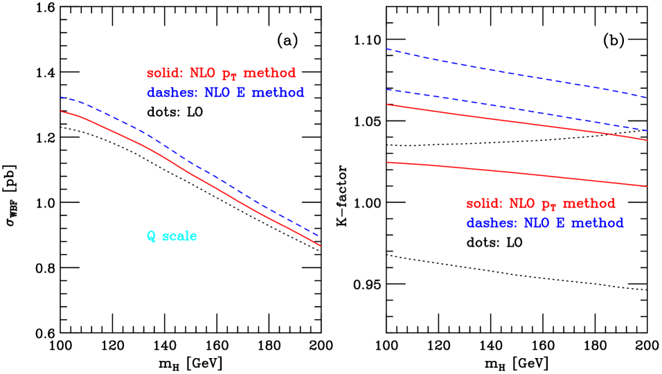
Figure 3: Effect of QCD radiative corrections on the Higgs boson production cross section via WBF, as a function of the Higgs boson mass, $m_{H}$. Results are given at LO (black dotted) and at NLO for the $p_{T}$-method (solid red) and the $E$-method (dashed blue) for defining tagging jets. Panel (a) gives the total cross section within the cuts of Eqs. (4.1)–(4.4). The corresponding scale dependence, for variation of $\mu_{R}$ and $\mu_{F}$ by a factor of 2, is shown in panel (b). See text for details.

Cross sections, within the cuts of Eqs. (4.1)–(4.4), are shown in Fig. 3(a), as a function of the Higgs boson mass, $m_{H}$. As for the total WBF cross section, the NLO effects are modest for the cross section within cuts, amounting to a 3-5% increase for the $p_{T}$-method of selecting tagging jets (solid red) and a 6-9% increase when the $E$-method is used. These $K$-factors, and their scale dependence, are shown in Fig. 3(b). Here the $K$-factor is defined as

$$K=\frac{\sigma(\mu_{R},\mu_{F})}{\sigma^{LO}(\mu_{F}=Q_{i})}\;,$$ (4.5)

i.e. the cross section is normalized to the LO cross section, determined with CTEQ6L1 parton distributions, and a factorization scale which is set to the virtuality of the weak boson which is attached to a given quark line.

We have investigated two general scale choices. First we consider the Higgs boson mass as the relevant hard scale, i.e. we set

$$\mu_{F}=\xi_{F}m_{H}\;,\qquad\qquad\mu_{R}=\xi_{R}m_{H}\;.$$ (4.6)

As a second option we consider the virtuality of the exchanged weak boson. Specifically, independent scales $Q_{i}$ are determined for radiative correction on the upper and the lower quark line, and we set

$$\mu_{Fi}=\xi_{F}Q_{i}\;,\qquad\qquad\mu_{Ri}=\xi_{R}Q_{i}\;.$$ (4.7)

This choice is motivated by the picture of WBF as two independent DIS events, with independent radiative corrections on the two electroweak boson vertices. In general we find the largest scale variations when we vary the renormalization scale and the factorization scale in the same direction. We only show results for this case, $\xi=\xi_{R}=\xi_{F}$, in the following. The curves in Fig. 3(b) correspond to the largest variations found for $\xi=1/2$ and $\xi=2$ when considering both scale choices simultaneously. The residual scale uncertainty is about $\pm 5$% at LO and reduces to below $\pm 2$% at NLO.

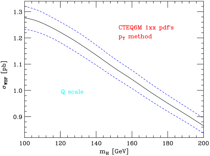
Figure 4: Variation of the total cross section, within cuts, due to errors in the parton distribution functions, as a function of $m_{H}$. The central solid line corresponds to the “best fit” CTEQ6M pdf, while the upper and lower curves define the pdf error band, which is determined from the 40 error eigenvectors in the CTEQ6M set (CTEQ6M101–CTEQ6M140), adding cross section deviations in quadrature.

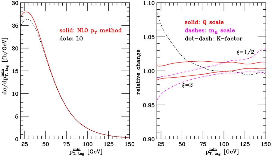
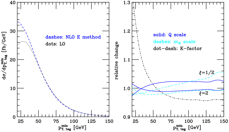
Figure 5: Transverse momentum distribution of the softer tagging jet for the the $p_{T}$-method (solid red) and the $E$-method (dashed blue) of defining tagging jets, for $m_{H}=120$ GeV. The right-hand panels give the $K$-factors (black dash-dotted line) and the scale variation of the NLO results. Solid colored curves correspond to $\mu_{F}=\mu_{R}=\xi Q_{i}$ and dashed colored curves are for $\mu_{F}=\mu_{R}=\xi m_{H}$ with $\xi=1/2$ and $2$.

In addition to missing higher order corrections, the theoretical error of the WBF cross section is dominated by uncertainties in the determination of the parton distribution functions. We have investigated this dependence by calculating the total Higgs boson cross section, within the cuts of Eqs. (4.1)–(4.4), for the 40 pdf’s in the CTEQ6Mxxx (xxx = 101–140) set. They correspond to extremal plus/minus variations in the directions of the 20 error eigenvectors of the Hessian of the CTEQ6M fitting parameters [15]. Adding the maximum deviations for each error eigenvector in quadrature, one obtains the blue dashed lines in Fig. 4, which define the pdf error band. We find a uniform $\pm 3.5\%$ pdf uncertainty of the total cross section over the entire range of $m_{H}$ shown.

Scale and pdf uncertainties exhibit little dependence on the Higgs boson mass. We therefore limit our investigation to a single, representative Higgs boson mass for the remaining discussion, which we take as $m_{H}=120$ GeV.

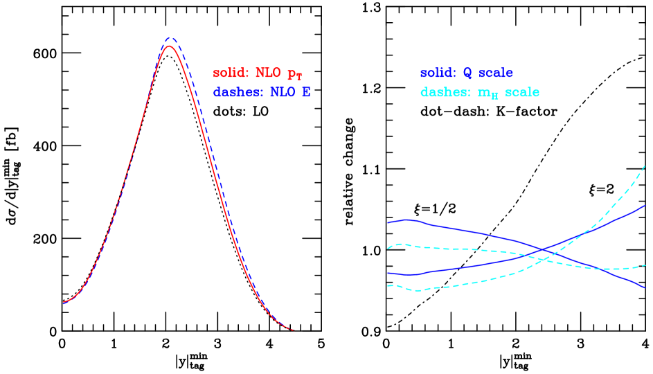
Figure 6: Higgs boson production cross section as a function of the smaller of the absolute value of the two tagging jet rapidities, $d\sigma/d|y|_{\rm tag}^{\rm min}$ (in fb, for $m_{H}=120$ GeV). Results are shown at LO (dotted black) and at NLO for the $p_{T}$-method (solid red) and the $E$-method (dashed blue) of defining tagging jets. The right-hand panel gives the $K$-factor (black dash-dotted line) and the scale variation of the NLO result for the $E$-method. Colored curves for the scale dependence are labeled as in Fig. 5.

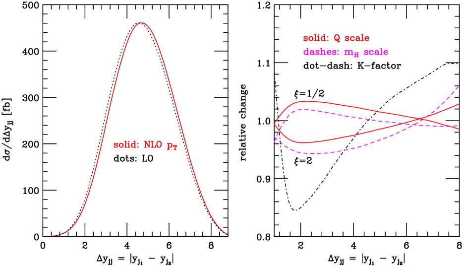
Figure 7: Rapidity separation of the two tagging jets for $m_{H}=120$ GeV. In the left-hand panel, $d\sigma/d\Delta y_{jj}$ (in fb) is shown at LO (dotted black) and at NLO (solid red), for the $p_{T}$-method of defining tagging jets. The right-hand panel gives the corresponding $K$-factor (black dash-dotted line) and the scale variation of the NLO results. Colored curves for the scale dependence are labeled as in Fig. 5.

While the scale dependence of the integrated Higgs boson production cross section is quite weak, the same need not be true for the shape of distributions which will be used to discriminate between Higgs boson signal and various backgrounds. Having a fully flexible NLO Monte Carlo program at hand, we can investigate this question. Crucial distributions for the detection efficiency of the signal are the transverse momentum and the rapidity of the tagging jets. In Fig. 5 the cross section is shown as a function of $p_{T,\,\rm tag}^{\rm min}$, the smaller of the two tagging jet transverse momenta. At LO, the tagging jets are uniquely defined, but at NLO one finds relatively large differences between the $p_{T}$-method (solid red curves in the top panels) and the $E$-method (dashed blue curves in bottom panels). The right-hand-side panels give the corresponding $K$-factors, as defined in Eq. (4.5), (black dash-dotted lines) and the ratio of NLO differential distributions for different scale choices. Shown are the ratios

$$R=\frac{d\sigma^{NLO}(\mu_{F}=\mu_{R}=Q_{i})}{d\sigma^{NLO}(\mu_{F}=\mu_{R}=\mu)}$$ (4.8)

for $\mu=2^{\pm 1}Q_{i}$ (solid lines) and $\mu=2^{\pm 1}m_{H}$ (dashed lines). While the $K$-factor is modest for the $p_{T}$-method, it reaches values around 1.3 in the threshold region for the $E$-method. This strong rise at NLO is due to hard forward gluon jets being misidentified as tagging jets in the $E$-method. This problem was recognized previously in parton shower Monte Carlo simulations and has prompted a preference for the $p_{T}$-method [18]. In spite of the large $K$-factor, however, the residual scale uncertainty is small, ranging from -4% to +2% for the $p_{T}$-method and -2% to +5% for the $E$-method.

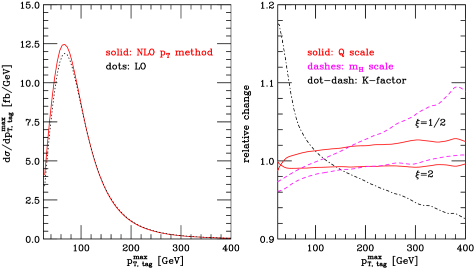
Figure 8: Transverse momentum distribution of the harder tagging jet, for $m_{H}=120$ GeV. In the left-hand panel, $d\sigma/dp_{T,\,\rm tag}^{\rm max}$ (in fb/GeV) is shown at LO (dotted black) and at NLO (solid red), for the $p_{T}$-method of defining tagging jets. The right-hand panel gives the corresponding $K$-factor (black dash-dotted line) and the scale variation of the NLO results. Colored curves for the scale dependence are labeled as in Fig. 5.

The more forward selection of tagging jets in the $E$-method is most obvious in the rapidity distributions of Figs. 6 and 7. In Fig. 6 the rapidity of the more central of the tagging jets, $|y|_{\rm tag}^{\rm min}$, is shown. At NLO, the tagging jets are slightly more forward than at tree level, leading to a $K$-factor which varies appreciably over phase space. This $|y|_{\rm tag}^{\rm min}$-dependence is shown in the right-hand panel for the $E$-method, together with the residual scale dependence at NLO. Again, scale variations of less than $\pm 4$% are found over virtually the entire phase space. For the $p_{T}$-method, similar scale variations arise, as shown in Fig. 7 for the rapidity separation between the two tagging jets, where the cuts of Eqs. (4.1)–(4.3) have been imposed. Figure 7 demonstrates that the wide separation of the tagging jets, which is important for rejection of QCD backgrounds, does survive at NLO. In fact, the tagging jet separation even increases slightly, making a separation cut like $\Delta y=|y_{j_{1}}-y_{j_{2}}|>4$ even more effective than at LO.

In all distributions considered so far, no clear preference emerges on whether to choose the weak-boson virtuality, $Q_{i}$, or $m_{H}$ as the hard scale. While both choices are acceptable, the transverse momentum distributions show somewhat smaller scale variations for $\mu=\xi Q_{i}$ than $\mu=\xi m_{H}$. The effect is most pronounced in the high $p_{T}$ tail of the tagging jet distributions. When considering $d\sigma/dp_{T,\rm tag}^{\rm max}$, as shown in Fig. 8, the scale variation increases to $+10$% at large $p_{T}$ when $\mu=\xi m_{H}$ is taken, while the same distribution for $\mu=\xi Q_{i}$ stays in a narrow $\pm 2$% band. This observation provides another reason for our default scale choice, $\mu=Q_{i}$.

Unlike the tagging jets considered so far, distributions of the Higgs decay products show little change in shape at NLO.

5 Conclusions

Weak-boson fusion processes will play an important role at future hadron colliders, most notably as a probe for electroweak symmetry breaking. For the particular case of Higgs boson production, we have presented a first analysis of the size and of the remaining uncertainties of NLO QCD corrections to jet distributions in WBF.

As for the inclusive WBF cross section, QCD corrections to distributions are of modest size, of order 10%, but occasionally they reach larger values. These corrections are strongly phase-space dependent for jet observables and an overall $K$-factor multiplying the LO distributions is not an adequate approximation. Within the phase-space region relevant for Higgs boson searches, we find differential $K$-factors as small as 0.9 or as large as 1.3. These corrections need to be taken into account for Higgs coupling measurements, and our NLO Monte Carlo program, or the recently released analogous program in the MCFM package [19], provide the necessary tools.

After inclusion of the one-loop QCD corrections, remaining uncertainties due to as yet uncalculated higher order terms, can be estimated by considering scale variations of the NLO cross section. Using the Higgs boson mass, $m_{H}$, and the weak-boson virtuality, $Q_{i}$, as potential hard scales, we find that these remaining scale dependencies are quite small. Varying renormalization or factorization scales by a factor of two away from these two central values results in typical changes of the NLO differential cross sections by $\pm 2$% or less. The uncertainty bands for $\mu=\xi m_{H}$ and $\mu=\xi Q_{i}$ typically overlap, yielding combined scale uncertainties of less than $\pm 3$% in most cases, occasionally rising up to order 5% at the edges of phase space. Moreover, the variation in different regions typically cancels in the integrated Higgs cross section, within cuts, leading to uncertainties due to higher order effects of $\pm 2$% (see Fig. 3), even when considering different hard scales. The remaining theoretical uncertainty on the measurable Higgs cross section, thus, is well below expected statistical errors, except for the $H\mbox{$\rightarrow$}WW$ search for Higgs masses around 170 GeV, where the high LHC rate allows statistical errors as low as 3%. In addition, pdf uncertainties for the total cross section are of order $\pm 3.5\%$ over the range 100 GeV $\leq m_{H}\leq$ 200 GeV. This means that the SM Higgs boson production cross section via WBF can be predicted, at present, with a theoretical error of about $\pm 4\%$.

The expected size of the LHC Higgs signal is enhanced slightly by the NLO QCD corrections. In addition to a $K$-factor slightly above unity this is due to a small shift of the tagging jets to higher rapidities, still well inside the detector coverage but moving the tagging jets slightly farther apart and hence allowing a better differentiation from QCD backgrounds.

The techniques described in this paper work in a very similar fashion for other weak-boson fusion processes. We are planning to extend our work to include also $W$ and $Z$ boson production via weak-boson fusion, and to make these programs generally available.

References

- [1] G. L. Bayatian et al., CMS Technical Proposal, report CERN/LHCC/94-38x (1994); R. Kinnunen and D. Denegri, CMS NOTE 1997/057; R. Kinnunen and A. Nikitenko, CMS TN/97-106; R. Kinnunen and D. Denegri, arXiv:hep-ph/9907291; V. Drollinger, T. Müller and D. Denegri, arXiv:hep-ph/0111312.
- [2] ATLAS Collaboration, ATLAS TDR, report CERN/LHCC/99-15 (1999); E. Richter-Was and M. Sapinski, Acta Phys. Polon. B 30, 1001 (1999); B. P. Kersevan and E. Richter-Was, Eur. Phys. J. C 25, 379 (2002) [arXiv:hep-ph/0203148].
- [3] D. Zeppenfeld, R. Kinnunen, A. Nikitenko and E. Richter-Was, Phys. Rev. D62, 013009 (2000) [arXiv:hep-ph/0002036]; D. Zeppenfeld, in Proc. of the APS/DPF/DPB Summer Study on the Future of Particle Physics (Snowmass 2001) ed. N. Graf, eConf C010630, P123 (2001) [arXiv:hep-ph/0203123]; A. Belyaev and L. Reina, JHEP 0208, 041 (2002) [arXiv:hep-ph/0205270].
- [4] D. Rainwater, D. Zeppenfeld and K. Hagiwara, Phys. Rev. D 59, 014037 (1999) [arXiv:hep-ph/9808468]; T. Plehn, D. Rainwater and D. Zeppenfeld, Phys. Rev. D61, 093005 (2000) [arXiv:hep-ph/9911385]; S. Asai et al., ATL-PHYS-2003-005.
- [5] D. Rainwater and D. Zeppenfeld, Phys. Rev. D 60, 113004 (1999) [Erratum-ibid. D 61, 099901 (2000)] [arXiv:hep-ph/9906218]; N. Kauer, T. Plehn, D. Rainwater and D. Zeppenfeld, Phys. Lett. B 503, 113 (2001) [arXiv:hep-ph/0012351]; C. M. Buttar, R. S. Harper and K. Jakobs, ATL-PHYS-2002-033; K. Cranmer et al., ATL-PHYS-2003-002 and ATL-PHYS-2003-007; S. Asai et al., ATL-PHYS-2003-005.
- [6] D. Rainwater and D. Zeppenfeld, JHEP 9712, 005 (1997) [arXiv:hep-ph/9712271].
- [7] O. J. Eboli and D. Zeppenfeld, Phys. Lett. B 495, 147 (2000) [arXiv:hep-ph/0009158]; B. Di Girolamo, A. Nikitenko, L. Neukermans, K. Mazumdar and D. Zeppenfeld, in arXiv:hep-ph/0203056.
- [8] T. Han and S. Willenbrock, Phys. Lett. B273, 167 (1991).
- [9] A. Djouadi, N. Spira and P. Zerwas, Phys. Lett. B264, 440 (1991); M. Spira, A. Djouadi, D. Graudenz and P.M. Zerwas, Nucl. Phys. B453, 17 (1995); S. Dawson, Nucl. Phys. B359, 283 (1991); S. Catani, D. de Florian, M. Grazzini and P. Nason, in arXiv:hep-ph/0204316.
- [10] S. Catani, D. de Florian and M. Grazzini, JHEP 0105, 025 (2001) [arXiv:hep-ph/0102227]; R. Harlander and W. Kilgore, Phys. Rev. D64, 013015 (2001) [arXiv:hep-ph/0102241]; R. Harlander and W. Kilgore, Phys. Rev. Lett. 88, 201801 (2002) [arXiv:hep-ph/0201206]; C. Anastasiou and K. Melnikov, Nucl. Phys. B646, 220 (2002) [arXiv:[hep-ph/0207004]; V. Ravindran, J. Smith and W.L. van Neerven, arXiv:hep-ph/0302135.
- [11] S. Catani and M. H. Seymour, Nucl. Phys. B 485, 291 (1997) [Erratum-ibid. B 510, 503 (1997)] [arXiv:hep-ph/9605323].
- [12] K. Hagiwara and D. Zeppenfeld, Nucl. Phys. B 274, 1 (1986); K. Hagiwara and D. Zeppenfeld, Nucl. Phys. B 313, 560 (1989).
- [13] G. P. Lepage, J. Comput. Phys. 27, 192 (1978).
- [14] M. Spira, Fortsch. Phys. 46, 203 (1998) [arXiv:hep-ph/9705337].
- [15] J. Pumplin, D. R. Stump, J. Huston, H. L. Lai, P. Nadolsky and W. K. Tung, JHEP 0207, 012 (2002) [arXiv:hep-ph/0201195].
- [16] S. Catani, Yu. L. Dokshitzer and B. R. Webber, Phys. Lett. B 285 291 (1992); S. Catani, Yu. L. Dokshitzer, M. H. Seymour and B. R. Webber, Nucl. Phys. B 406 187 (1993); S. D. Ellis and D. E. Soper, Phys. Rev. D48 3160 (1993).
- [17] G. C. Blazey et al., arXiv:hep-ex/0005012.
- [18] V. Cavasinni, D. Costanzo, E. Mazzoni and I. Vivarelli, ATL-PHYS-2002-010.
- [19] J. Campbell and K. Ellis, MCFM - Monte Carlo for FeMtobarn processes, http://mcfm.fnal.gov/.