NEUTRINO MASS, FLAVOUR AND CP VIOLATION

Abstract

In this talk I discuss the connection between neutrino mass, flavour and CP violation. I focus on three neutrino patterns of neutrino masses and mixing angles, and the corresponding Majorana mass matrices. I discuss the see-saw mechanism, and show how it may be applied in a very natural way to give a neutrino mass hierarchy with large atmospheric and solar angles by assuming sequential right-handed neutrino dominance. I then distinguish between heavy sequential dominance and light sequential dominance, and show how lepton flavour violation in the CMSSM provides a way to discriminate between these two possibilities. I also show that for a well motivated class of light sequential dominance models there is a link between leptogenesis and CP violation measurable in neutrino oscillation experiments.

Department of Physics and Astronomy,
University of Southampton, Southampton SO17 1BJ, U.K. E-mail: sfk@hep.phys.soton.ac.uk

1 NEUTRINO MASSES AND MIXING ANGLES

There is by now strong evidence for neutrino oscillations in both the atmospheric and solar neutrino sectors ^{?,?,?,?,?,?,?)}. The minimal neutrino sector required to account for the atmospheric and solar neutrino oscillation data consists of three light physical neutrinos with left-handed flavour eigenstates, $\nu_{e}$, $\nu_{\mu}$, and $\nu_{\tau}$, defined to be those states that share the same electroweak doublet as the left-handed charged lepton mass eigenstates. Within the framework of three–neutrino oscillations, the neutrino flavor eigenstates $\nu_{e}$, $\nu_{\mu}$, and $\nu_{\tau}$ are related to the neutrino mass eigenstates $\nu_{1}$, $\nu_{2}$, and $\nu_{3}$ with mass $m_{1}$, $m_{2}$, and $m_{3}$, respectively, by a $3\times 3$ unitary matrix $U$ ^?,?,?)

$$\left(\begin{array}[]{c}\nu_{e}\\ \nu_{\mu}\\ \nu_{\tau}\end{array}\\ \right)=\left(\begin{array}[]{ccc}U_{e1}&U_{e2}&U_{e3}\\ U_{\mu 1}&U_{\mu 2}&U_{\mu 3}\\ U_{\tau 1}&U_{\tau 2}&U_{\tau 3}\\ \end{array}\right)\left(\begin{array}[]{c}\nu_{1}\\ \nu_{2}\\ \nu_{3}\end{array}\\ \right)\;.$$ (1)

Assuming the light neutrinos are Majorana, $U$ can be parameterized in terms of three mixing angles $\theta_{ij}$ and three complex phases $\delta_{ij}$. A unitary matrix has six phases but three of them are removed by the phase symmetry of the charged lepton Dirac masses. Since the neutrino masses are Majorana there is no additional phase symmetry associated with them, unlike the case of quark mixing where a further two phases may be removed. The neutrino mixing matrix may be parametrised by a product of three complex Euler rotations,

$$U=U_{23}U_{13}U_{12}$$ (2)

where

$$U_{23}=\left(\begin{array}[]{ccc}1&0&0\\ 0&c_{23}&s_{23}e^{-i\delta_{23}}\\ 0&-s_{23}e^{i\delta_{23}}&c_{23}\\ \end{array}\right)$$ (3)

$$U_{13}=\left(\begin{array}[]{ccc}c_{13}&0&s_{13}e^{-i\delta_{13}}\\ 0&1&0\\ -s_{13}e^{i\delta_{13}}&0&c_{13}\\ \end{array}\right)$$ (4)

$$U_{12}=\left(\begin{array}[]{ccc}c_{12}&s_{12}e^{-i\delta_{12}}&0\\ -s_{12}e^{i\delta_{12}}&c_{12}&0\\ 0&0&1\\ \end{array}\right)$$ (5)

where $c_{ij}=\cos\theta_{ij}$ and $s_{ij}=\sin\theta_{ij}$. Note that the allowed range of the angles is $0\leq\theta_{ij}\leq\pi/2$. Since we have assumed that the neutrinos are Majorana, there are two extra phases, but only one combination $\delta=\delta_{13}-\delta_{23}-\delta_{12}$ affects oscillations.

Ignoring phases, the relation between the neutrino flavor eigenstates $\nu_{e}$, $\nu_{\mu}$, and $\nu_{\tau}$ and the neutrino mass eigenstates $\nu_{1}$, $\nu_{2}$, and $\nu_{3}$ is just given as a product of three Euler rotations as depicted in Fig.1.

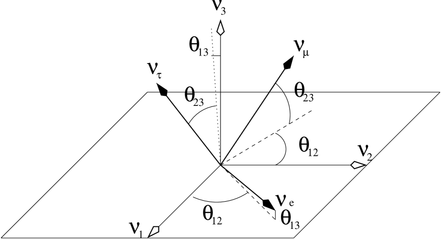
Figure 1: A graphical illustration of the neutrino mixing angles. This figure ignores the phases so that the neutrino mixing matrix is constructed as a product of three Euler rotations $U=R_{23}R_{13}R_{12}$. The atmospheric angle is $\theta_{23}\approx\pi/4$, the CHOOZ angle is $\theta_{13}\buildrel<\over{{}_{\sim}}0.2$, and the solar angle is $\theta_{12}\approx\pi/6$.

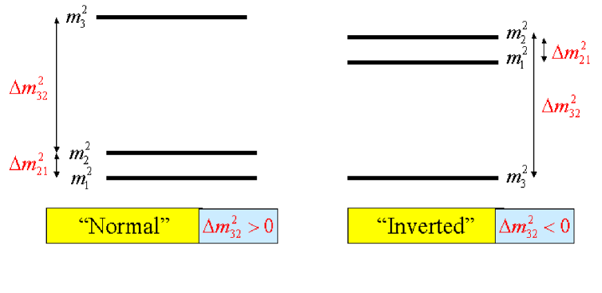
Figure 2: Alternative neutrino mass patterns that are consistent with neutrino oscillation explanations of the atmospheric and solar data. The absolute scale of neutrino masses is not fixed by oscillation data and the lightest neutrino mass may vary from 0.0-0.23 eV.

There are basically two patterns of neutrino mass squared orderings consistent with the atmospheric and solar data as shown in Fig.2.

It is clear that neutrino oscillations, which only depend on $\Delta m_{ij}^{2}\equiv m_{i}^{2}-m_{j}^{2}$, give no information about the absolute value of the neutrino mass squared eigenvalues $m_{i}^{2}$ in Fig.2. Recent results from the 2df galaxy redshift survey and WMAP indicate that $\sum m_{i}<0.69{\rm eV}(95\%C.L.)$ under certain mild assumptions ^?,?). Combined with the solar and atmospheric oscillation data this brackets the heaviest neutrino mass to be in the approximate range 0.05-0.23 eV. The fact that the mass of the heaviest neutrino is known to within an order of magnitude represents remarkable progress in neutrino physics over recent years.

2 CONSTRUCTING THE NEUTRINO MIXING MATRIX

From a model building perspective the neutrino and charged lepton masses are given by the eigenvalues of a complex charged lepton mass matrix $m^{E}_{LR}$ and a complex symmetric neutrino Majorana matrix $m_{LL}$, obtained by diagonalising these mass matrices,

$$V^{E_{L}}m^{E}_{LR}{V^{E_{R}}}^{\dagger}=\left(\begin{array}[]{ccc}m_{e}&0&0\\ 0&m_{\mu}&0\\ 0&0&m_{\tau}\end{array}\right)$$ (6)

$$V^{\nu_{L}}m_{LL}{V^{\nu_{L}}}^{T}=\left(\begin{array}[]{ccc}m_{1}&0&0\\ 0&m_{2}&0\\ 0&0&m_{3}\end{array}\right)$$ (7)

where $V^{E_{L}}$, $V^{E_{R}}$, $V^{\nu_{L}}$ are unitary tranformations on the left-handed charged lepton fields $E_{L}$, right-handed charged lepton fields $E_{R}$, and left-handed neutrino fields $\nu_{L}$ which put the mass matrices into diagonal form with real eigenvalues.

The neutrino mixing matrix is then constructed by

$$U=V^{E_{L}}{V^{\nu_{L}}}^{\dagger}$$ (8)

The neutrino mixing matrix is constructed in Eq.8 as a product of a unitary matrix from the charged lepton sector $V^{E_{L}}$ and a unitary matrix from the neutrino sector ${V^{\nu_{L}}}^{\dagger}$. Each of these unitary matrices may be parametrised by its own mixing angles and phases analagous to the parameters of $U$. As shown in ^?) the $U$ matrix can be expanded in terms of neutrino and charged lepton mixing angles and phases to leading order in the charged lepton mixing angles which are assumed to be small,

$$s_{23}e^{-i\delta_{23}} \approx s_{23}^{\nu_{L}}e^{-i\delta_{23}^{\nu_{L}}}-\theta_{23}^{E_{L}}c_{23}^{\nu_{L}}e^{-i\delta_{23}^{E_{L}}}$$ (9)

$$\theta_{13}e^{-i\delta_{13}} \approx \theta_{13}^{\nu_{L}}e^{-i\delta_{13}^{\nu_{L}}}-\theta_{13}^{E_{L}}c_{23}^{\nu_{L}}e^{-i\delta_{13}^{E_{L}}}$$ (10)

$$+ \theta_{12}^{E_{L}}s_{23}^{\nu_{L}}e^{i(-\delta_{23}^{\nu_{L}}-\delta_{12}^{E_{L}})}$$

$$s_{12}e^{-i\delta_{12}} \approx s_{12}^{\nu_{L}}e^{-i\delta_{12}^{\nu_{L}}}+\theta_{23}^{E_{L}}s_{12}^{\nu_{L}}e^{-i\delta_{12}^{\nu_{L}}}$$ (11)

$$+ \theta_{13}^{E_{L}}c_{12}^{\nu_{L}}s_{23}^{\nu_{L}}e^{i(\delta_{23}^{\nu_{L}}-\delta_{13}^{E_{L}})}$$

$$- \theta_{12}^{E_{L}}c_{23}^{\nu_{L}}c_{12}^{\nu_{L}}e^{-i\delta_{12}^{E_{L}}}$$

Clearly $\theta_{13}$ receives important contributions not just from $\theta_{13}^{\nu_{L}}$, but also from the charged lepton angles $\theta_{12}^{E_{L}}$, and $\theta_{13}^{E_{L}}$. In models where $\theta_{13}^{\nu_{L}}$ is extremely small, $\theta_{13}$ may originate almost entirely from the charged lepton sector. Charged lepton contributions could also be important in models where $\theta_{12}^{\nu_{L}}=\pi/4$, since charged lepton mixing angles may allow consistency with the LMA MSW solution. Such effects are important for the inverted hierarchy model ^?,?).

3 NEUTRINO MAJORANA MASS MATRICES

For many (but not all) purposes it is convenient to forget about the division between charged lepton and neutrino mixing angles and work in a basis where the charged lepton mass matrix is diagonal. Then the neutrino mixing angles and phases simply correspond to the neutrino ones. In this special basis the mass matrix is given from Eq.7 and Eq.8 as

$$m_{LL}=U\left(\begin{array}[]{ccc}m_{1}&0&0\\ 0&m_{2}&0\\ 0&0&m_{3}\end{array}\right)U^{T}$$ (12)

For a given assumed form of $U$ and set of neutrino masses $m_{i}$ one may use Eq.12 to “derive” the form of the neutrino mass matrix $m_{LL}$, and this results in the candidate mass matrices in Table 1 ^?).

Table 1: Leading order low energy neutrino Majorana mass matrices $m_{LL}$ consistent with large atmospheric and solar mixing angles, classified according to the rate of neutrinoless double beta decay and the pattern of neutrino masses.

	Type I	Type II
	Small $\beta\beta_{0\nu}$	Large $\beta\beta_{0\nu}$
A	$\beta\beta_{0\nu}\buildrel<\over{{}_{\sim}}0.0082$ eV
Normal hierarchy
$m_{1}^{2},m_{2}^{2}\ll m_{3}^{2}$	$\left(\begin{array}[]{ccc}0&0&0\\ 0&1&1\\ 0&1&1\\ \end{array}\right)\frac{m}{2}$	–
B	$\beta\beta_{0\nu}\buildrel<\over{{}_{\sim}}0.0082$ eV	$\beta\beta_{0\nu}\buildrel>\over{{}_{\sim}}0.0085$ eV
Inverted hierarchy
$m_{1}^{2}\approx m_{2}^{2}\gg m_{3}^{2}$	$\left(\begin{array}[]{ccc}0&1&1\\ 1&0&0\\ 1&0&0\\ \end{array}\right)\frac{m}{\sqrt{2}}$	$\left(\begin{array}[]{ccc}1&0&0\\ 0&\frac{1}{2}&\frac{1}{2}\\ 0&\frac{1}{2}&\frac{1}{2}\\ \end{array}\right)m$
C		$\beta\beta_{0\nu}\buildrel>\over{{}_{\sim}}0.035$ eV
Approximate degeneracy		diag(1,1,1)m
$m_{1}^{2}\approx m_{2}^{2}\approx m_{3}^{2}$	$\left(\begin{array}[]{ccc}0&\frac{1}{\sqrt{2}}&\frac{1}{\sqrt{2}}\\ \frac{1}{\sqrt{2}}&\frac{1}{2}&\frac{1}{2}\\ \frac{1}{\sqrt{2}}&\frac{1}{2}&\frac{1}{2}\\ \end{array}\right)m$	$\left(\begin{array}[]{ccc}1&0&0\\ 0&0&1\\ 0&1&0\\ \end{array}\right)m$

In Table 1 the mass matrices are classified into two types:

Type I - small neutrinoless double beta decay

Type II - large neutrinoless double beta decay

They are also classified into the limiting cases consistent with the mass squared orderings in Fig.2:

A - Normal hierarchy $m_{1}^{2},m_{2}^{2}\ll m_{3}^{2}$

B - Inverted hierarchy $m_{1}^{2}\approx m_{2}^{2}\gg m_{3}^{2}$

C - Approximate degeneracy $m_{1}^{2}\approx m_{2}^{2}\approx m_{3}^{2}$

Thus according to our classification there is only one neutrino mass matrix consistent with the normal neutrino mass hierarchy which we call Type IA, corresponding to the leading order neutrino masses of the form $m_{i}=(0,0,m)$. For the inverted hierarchy there are two cases, Type IB corresponding to $m_{i}=(m,-m,0)$ or Type IIB corresponding to $m_{i}=(m,m,0)$. For the approximate degeneracy cases there are three cases, Type IC correponding to $m_{i}=(m,-m,m)$ and two examples of Type IIC corresponding to either $m_{i}=(m,m,m)$ or $m_{i}=(m,m,-m)$.

At present experiment allows any of the matrices in Table 1. In future it will be possible to uniquely specify the neutrino matrix in the following way:

1. Neutrinoless double beta effectively measures the 11 element of the mass matrix $m_{LL}$ corresponding to

$$\beta\beta_{0\nu}\equiv\sum_{i}U_{ei}^{2}m_{i}$$ (13)

and is clearly capable of resolving Type I from Type II cases according to the bounds given in Table 1 ^?). There has been a recent claim of a signal in neutrinoless double beta decay correponding to $\beta\beta_{0\nu}=0.11-0.56$ eV at 95% C.L. ^?). However this claim has been criticised by two groups ^?), ^?) and in turn this criticism has been refuted ^?). Since the Heidelberg-Moscow experiment has almost reached its full sensitivity, we may have to wait for a next generation experiment such as GENIUS ^?) which is capable of pushing down the sensitivity to 0.01 eV to resolve this question.

2. A neutrino factory will measure the sign of $\Delta m_{32}^{2}$ and resolve A from B ^?).

3. Tritium beta decay experiments are sensitive to C since they measure the “electron neutrino mass” defined by

$$|m_{\nu_{e}}|\equiv\sum_{i}|U_{ei}|^{2}|m_{i}|.$$ (14)

For example the KATRIN ^?) experiment has a proposed sensitivity of 0.35 eV. As already mentioned the galaxy power spectrum combined with solar and atmospheric oscillation data already limits the degenerate neutrino mass to be less than about 0.6 eV, and this limit is also expected to improve in the future. Also it is worth mentioning that in future it may be possible to measure neutrino masses from gamma ray bursts using time of flight techniques in principle down to 0.001 eV ^?).

Type IIB and C involve small fractional mass splittings $|\Delta m_{ij}^{2}|\ll m^{2}$ which are unstable under radiative corrections, and even the most natural Type IC case is difficult to implement. Types IA and IB seem to be the most natural and later we shall focus on the normal hierarchy Type IA,

$$m_{LL}\sim\left(\begin{array}[]{ccc}0&0&0\\ 0&1&1\\ 0&1&1\\ \end{array}\right)\frac{m}{2}$$ (15)

However even Type IA models appear to have some remaining naturalness problem since $m_{3}\sim\sqrt{|\Delta m_{32}^{2}|}\sim 5.10^{-2}$ eV and $m_{2}\sim\sqrt{|\Delta m_{21}^{2}|}\sim 7.10^{-3}$ eV, compared to the natural expectation $m_{2}\sim m_{3}$. The question may be phrased in technical terms as one of understanding why the sub-determinant of the mass matrix in Eq.15 is small:

$$det\left(\begin{array}[]{cc}m_{22}&m_{23}\\ m_{23}&m_{33}\\ \end{array}\right)\ll m^{2}.$$ (16)

4 THE SEE-SAW MASS MECHANISM

Before discussing the see-saw mechanism it is worth first reviewing the different types of neutrino mass that are possible. So far we have been assuming that neutrino masses are Majorana masses of the form

$$m_{LL}\overline{\nu_{L}}\nu_{L}^{c}$$ (17)

where $\nu_{L}$ is a left-handed neutrino field and $\nu_{L}^{c}$ is the CP conjugate of a left-handed neutrino field, in other words a right-handed antineutrino field. Such Majorana masses are possible to since both the neutrino and the antineutrino are electrically neutral and so Majorana masses are not forbidden by electric charge conservation. For this reason a Majorana mass for the electron would be strictly forbidden. Majorana neutrino masses “only” violate lepton number conservation. If we introduce right-handed neutrino fields then there are two sorts of additional neutrino mass terms that are possible. There are additional Majorana masses of the form

$$M_{RR}\overline{\nu_{R}}\nu_{R}^{c}$$ (18)

where $\nu_{R}$ is a right-handed neutrino field and $\nu_{R}^{c}$ is the CP conjugate of a right-handed neutrino field, in other words a left-handed antineutrino field. In addition there are Dirac masses of the form

$$m_{LR}\overline{\nu_{L}}\nu_{R}.$$ (19)

Such Dirac mass terms conserve lepton number, and are not forbidden by electric charge conservation even for the charged leptons and quarks.

In the Standard Model Dirac mass terms for charged leptons and quarks are generated from Yukawa couplings to a Higgs doublet whose vacuum expectation value gives the Dirac mass term. Neutrino masses are zero in the Standard Model because right-handed neutrinos are not present, and also because the Majorana mass terms in Eq.17 require Higgs triplets in order to be generated at the renormalisable level (although non-renormalisable operators can be written down. Higgs triplets are phenomenologically disfavoured so the simplest way to generate neutrino masses from a renormalisable theory is to introduce right-handed neutrinos. Once this is done then the types of neutrino mass discussed in Eqs.18,19 (but not Eq.17 since we have not introduced Higgs triplets) are permitted, and we have the mass matrix

$$\left(\begin{array}[]{cc}\overline{\nu_{L}}&\overline{\nu^{c}_{R}}\end{array}\\ \right)\left(\begin{array}[]{cc}0&m_{LR}\\ m_{LR}^{T}&M_{RR}\\ \end{array}\right)\left(\begin{array}[]{c}\nu_{L}^{c}\\ \nu_{R}\end{array}\\ \right)$$ (20)

Since the right-handed neutrinos are electroweak singlets the Majorana masses of the right-handed neutrinos $M_{RR}$ may be orders of magnitude larger than the electroweak scale. In the approximation that $M_{RR}\gg m_{LR}$ the matrix in Eq.20 may be diagonalised to yield effective Majorana masses of the type in Eq.17,

$$m_{LL}=m_{LR}M_{RR}^{-1}m_{LR}^{T}$$ (21)

This is the see-saw mechanism . It not only generates Majorana mass terms of the type $m_{LL}$, but also naturally makes them smaller than the Dirac mass terms by a factor of $m_{LR}/M_{RR}\ll 1$. One can think of the heavy right-handed neutrinos as being integrated out to give non-renormalisable Majorana operators suppressed by the heavy mass scale $M_{RR}$.

In a realistic model with three left-handed neutrinos and three right-handed neutrinos the Dirac masses $m_{LR}$ are a $3\times 3$ (complex) matrix and the heavy Majorana masses $M_{RR}$ form a separate $3\times 3$ (complex symmetric) matrix. The light effective Majorana masses $m_{LL}$ are also a $3\times 3$ (complex symmetric) matrix and continue to be given from Eq.21 which is now interpreted as a matrix product. From a model building perspective the fundamental parameters which must be input into the see-saw mechanism are the Dirac mass matrix $m_{LR}$ and the heavy right-handed neutrino Majorana mass matrix $M_{RR}$. The light effective left-handed Majorana mass matrix $m_{LL}$ arises as an output according to the see-saw formula in Eq.21. The goal of see-saw model building is therefore to choose input see-saw matrices $m_{LR}$ and $M_{RR}$ that will give rise to one of the successful matrices $m_{LL}$ in Table 1.

5 SEQUENTIAL RIGHT HANDED NEUTRINO DOMINANCE

With three left-handed neutrinos and three right-handed neutrinos the Dirac masses $m_{LR}$ are a $3\times 3$ (complex) matrix and the heavy Majorana masses $M_{RR}$ form a separate $3\times 3$ (complex symmetric) matrix. The light effective Majorana masses $m_{LL}$ are also a $3\times 3$ (complex symmetric) matrix and continue to be given from Eq.21 which is now interpreted as a matrix product. From a model building perspective the fundamental parameters which must be input into the see-saw mechanism are the Dirac mass matrix $m_{LR}$ and the heavy right-handed neutrino Majorana mass matrix $M_{RR}$. The light effective left-handed Majorana mass matrix $m_{LL}$ arises as an output according to the see-saw formula in Eq.21. The goal of see-saw model building is therefore to choose input see-saw matrices $m_{LR}$ and $M_{RR}$ that will give rise to one of the successful matrices $m_{LL}$ in Table 1.

We now show how the input see-saw matrices can be simply chosen to give the Type IA matrix in Eq.15, with the property of a naturally small sub-determinant in Eq.16 using a mechanism first suggested in ^?). The idea was developed in ^?) where it was called single right-handed neutrino dominance (SRHND) . SRHND was first successfully applied to the LMA MSW solution in ^?).

The SRHND mechanism is most simply described assuming three right-handed neutrinos in the basis where the right-handed neutrino mass matrix is diagonal although it can also be developed in other bases ^?,?). In this basis we write the input see-saw matrices as

$$M_{RR}=\left(\begin{array}[]{ccc}X^{\prime}&0&0\\ 0&X&0\\ 0&0&Y\end{array}\right)$$ (22)

$$m_{LR}=\left(\begin{array}[]{ccc}a^{\prime}&a&d\\ b^{\prime}&b&e\\ c^{\prime}&c&f\end{array}\right)$$ (23)

In ^?) it was suggested that one of the right-handed neutrinos may dominante the contribution to $m_{LL}$ if it is lighter than the other right-handed neutrinos. The dominance condition was subsequently generalised to include other cases where the right-handed neutrino may be heavier than the other right-handed neutrinos but dominates due to its larger Dirac mass couplings ^?). In any case the dominant neutrino may be taken to be the third one without loss of generality. Assuming SRHND then Eqs.21, 22, 23 give, retaining only the leading dominant right-handed neutrino contributions proportional to $1/Y$,

$$m_{LL}\approx\left(\begin{array}[]{ccc}\frac{d^{2}}{Y}&\frac{de}{Y}&\frac{df}{Y}\\ .&\frac{e^{2}}{Y}&\frac{ef}{Y}\\ .&.&\frac{f^{2}}{Y}\end{array}\right)$$ (24)

If the Dirac mass couplings satisfy the condition $d\ll e\approx f$ ^?) then the matrix in Eq.24 resembles the Type IA matrix in Eq.15, and furthermore has a naturally small sub-determinant as in Eq.16. The neutrino mass spectrum consists of one neutrino with mass $m_{3}\approx(e^{2}+f^{2})/Y$ and two approximately massless neutrinos ^?). The atmospheric angle is $\tan\theta_{23}\approx e/f$ ^?). It was pointed out that small perturbations from the sub-dominant right-handed neutrinos can then lead to a small solar neutrino mass splitting ^?).

It was subsequently shown how to account for the LMA MSW solution with a large solar angle ^?) by careful consideration of the sub-dominant contributions. One of the examples considered in ^?) is when the right-handed neutrinos dominate sequentially,

$$\frac{|e^{2}|,|f^{2}|,|ef|}{Y}\gg\frac{|xy|}{X}\gg\frac{|x^{\prime}y^{\prime}|}{X^{\prime}}$$ (25)

where $x,y\in a,b,c$ and $x^{\prime},y^{\prime}\in a^{\prime},b^{\prime},c^{\prime}$. Assuming SRHND with sequential sub-dominance as in Eq.25, then Eqs.21, 22, 23 give

$$m_{LL}\approx\left(\begin{array}[]{ccc}\frac{a^{2}}{X}+\frac{d^{2}}{Y}&\frac{ab}{X}+\frac{de}{Y}&\frac{ac}{X}+\frac{df}{Y}\\ .&\frac{b^{2}}{X}+\frac{e^{2}}{Y}&\frac{bc}{X}+\frac{ef}{Y}\\ .&.&\frac{c^{2}}{X}+\frac{f^{2}}{Y}\end{array}\right)$$ (26)

where the contribution from the first right-handed neutrino may be neglected according to Eq.25. This was shown to lead to a full neutrino mass hierarchy

$$m_{1}^{2}\ll m_{2}^{2}\ll m_{3}^{2}$$ (27)

and, ignoring phases, the solar angle only depends on the sub-dominant couplings and is given by $\tan\theta_{12}\approx a/(c_{23}b-s_{23}c)$ ^?). The simple requirement for large solar angle is then $a\sim b-c$ ^?).

Including phases the neutrino masses are given to leading order in $m_{2}/m_{3}$ by diagonalising the mass matrix in Eq.26 using the analytic proceedure described in ^?),

$$m_{1} \sim O(\frac{x^{\prime}y^{\prime}}{X^{\prime}}v_{2}^{2})$$ (28)

$$m_{2} \approx \frac{|a|^{2}}{Xs_{12}^{2}}v_{2}^{2}$$ (29)

$$m_{3} \approx \frac{|e|^{2}+|f|^{2}}{Y}v_{2}^{2}$$ (30)

where $v_{2}$ is a Higgs vacuum expectation value (vev) associated with the (second) Higgs doublet that couples to the neutrinos and $s_{12}=\sin\theta_{12}$ given below. Note that with SD each neutrino mass is generated by a separate right-handed neutrino, and the sequential dominance condition naturally results in a neutrino mass hierarchy $m_{1}\ll m_{2}\ll m_{3}$. The neutrino mixing angles are given to leading order in $m_{2}/m_{3}$ by,

$$\tan\theta_{23} \approx \frac{|e|}{|f|}$$ (31)

$$\tan\theta_{12} \approx \frac{|a|}{c_{23}|b|\cos(\tilde{\phi}_{b})-s_{23}|c|\cos(\tilde{\phi}_{c})}$$ (32)

$$\theta_{13} \approx e^{i(\tilde{\phi}+\phi_{a}-\phi_{e})}\frac{|a|(e^{*}b+f^{*}c)}{[|e|^{2}+|f|^{2}]^{3/2}}\frac{Y}{X}$$ (33)

where we have written some (but not all) complex Yukawa couplings as $x=|x|e^{i\phi_{x}}$. The phase $\delta$ is fixed to give a real angle $\theta_{12}$ by,

$$c_{23}|b|\sin(\tilde{\phi}_{b})\approx s_{23}|c|\sin(\tilde{\phi}_{c})$$ (34)

where

$$\tilde{\phi}_{b} \equiv \phi_{b}-\phi_{a}-\tilde{\phi}+\delta,$$

$$\tilde{\phi}_{c} \equiv \phi_{c}-\phi_{a}+\phi_{e}-\phi_{f}-\tilde{\phi}+\delta$$ (35)

The phase $\tilde{\phi}$ is fixed to give a real angle $\theta_{13}$ by,

$$\tilde{\phi}\approx\phi_{e}-\phi_{a}-\phi_{\rm COSMO}$$ (36)

where

$$\phi_{\rm COSMO}=\arg(e^{*}b+f^{*}c).$$ (37)

is the leptogenesis phase corresponding to the interference diagram involving the lightest and next-to-lightest right-handed neutrinos ^?).

6 LIGHT OR HEAVY SEQUENTIAL DOMINANCE?

Assuming sequential dominance described in the previous section, there is still an ambiguity regarding the mass ordering of the heavy Majorana right-handed neutrinos. There are two extreme possibilities called heavy sequential dominance (HSD) and light sequential dominance (LSD). In HSD the dominant right-handed neutrino (always denoted by Majorana mass $Y$) is the heaviest,

$$X^{\prime}\ll X\ll Y$$ (38)

Then assuming that the 33 element of the neutrino Yukawa matrix is of order unity, this leads to a “lop-sided” Yukawa matrix, since $e\sim f\sim 1$,

$$M^{HSD}_{RR}=\left(\begin{array}[]{ccc}X^{\prime}&0&0\\ 0&X&0\\ 0&0&Y\end{array}\right)$$ (39)

$${Y_{\nu}}^{HSD}_{LR}=\left(\begin{array}[]{ccc}a^{\prime}&a&d\\ b^{\prime}&b&e\\ c^{\prime}&c&f\end{array}\right)$$ (40)

On the other hand in LSD, the dominant right-handed neutrino of mass $Y$ is by definition the lightest one,

$$Y\ll X\ll X^{\prime}$$ (41)

Then still assuming that the 33 element of the neutrino Yukawa matrix is of order unity, this leads to a “quark-like” Yukawa matrix, since in this case $e\sim f\ll 1$ consistent with a symmetrical structure with no large off-diagonal elements, after reordering the right-handed neutrinos,

$$M^{LSD}_{RR}=\left(\begin{array}[]{ccc}Y&0&0\\ 0&X&0\\ 0&0&X^{\prime}\end{array}\right)$$ (42)

$${Y_{\nu}}^{HSD}_{LR}=\left(\begin{array}[]{ccc}d&a&a^{\prime}\\ e&b&b^{\prime}\\ f&c&c^{\prime}\end{array}\right)$$ (43)

Note that in LSD, the right-handed neutrino of mass $X^{\prime}$ is irrelevant for neutrino masses and mixings, as well as leptogenesis. For all practical purposes, the LSD model reduces to an effective two right-handed neutrino model.

7 LEPTON FLAVOUR VIOLATION IN THE CMSSM WITH SEQUENTIAL DOMINANCE

At leading order in a mass insertion approximation the branching fractions of LFV processes are given by

$${\rm BR}(l_{i}\rightarrow l_{j}\gamma)\approx\frac{\alpha^{3}}{G_{F}^{2}}f(M_{2},\mu,m_{\tilde{\nu}})|m_{\tilde{L}_{ij}}^{2}|^{2}\tan^{2}\beta$$ (44)

where $l_{1}=e,l_{2}=\mu,l_{3}=\tau$, and where the off-diagonal slepton doublet mass squared is given in the leading log approximation (LLA) by

$$m_{\tilde{L}_{ij}}^{2(LLA)}\approx-\frac{(3m_{0}^{2}+A_{0}^{2})}{8\pi^{2}}C_{ij}$$ (45)

where the leading log coefficients relevant for $\mu\rightarrow e\gamma$ and $\tau\rightarrow\mu\gamma$ are given approximately as

$$C_{21} = ab\ln\frac{M_{U}}{X}+de\ln\frac{M_{U}}{Y}$$

$$C_{32} = bc\ln\frac{M_{U}}{X}+ef\ln\frac{M_{U}}{Y}$$ (46)

We have performed a global analysis of LFV in the constrained minimal supersymmetric standard model (CMSSM) for the case of sequential dominance, focussing on the two cases of HSD and LSD ^?). We parametrise the matrices ^?) in a quite general way consistent with sequential dominance. The numerical results we show here are for a particular case of HSD and LSD defined below

$$M^{HSD}_{RR} = \left(\begin{array}[]{ccc}-&0&0\\ 0&\lambda^{3}&0\\ 0&0&1\end{array}\right)3.10^{14}GeV$$ (50)

$$Y^{\nu HSD}_{LR} = \left(\begin{array}[]{ccc}-&a_{12}\lambda^{2}&0\\ -&a_{22}\lambda^{2}&1\\ -&a_{32}\lambda^{2}&1\end{array}\right)$$ (54)

$$M^{LSD}_{RR} = \left(\begin{array}[]{ccc}\lambda^{6}&0&0\\ 0&\lambda^{3}&0\\ 0&0&\gg 1\end{array}\right)3\times 10^{14}GeV$$ (58)

$$Y^{\nu LSD}_{LR} = \left(\begin{array}[]{ccc}0&a_{12}\lambda^{2}&-\\ \lambda^{3}&a_{22}\lambda^{2}&-\\ \lambda^{3}&a_{32}\lambda^{2}&1\end{array}\right)$$ (62)

where $a_{ij}$ are order unity coefficients, $\lambda=\sqrt{\Delta m_{21}^{2}/\Delta m_{32}^{2}}\approx 0.15$.

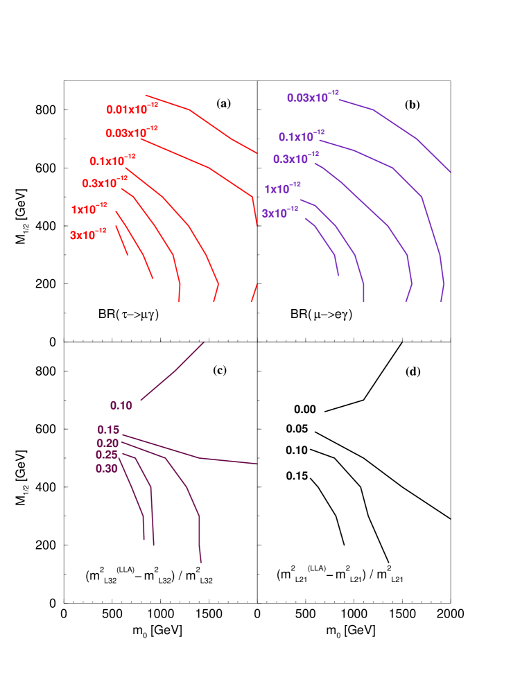
Figure 4: The upper panels show the predictions for the branching fraction for (a) $\tau\rightarrow\mu\gamma$ and (b) $\mu\rightarrow e\gamma$ for LSD using the parameters described in the text. The lower panels (c), (d) show the fractional error $\Delta_{ij}$, defined in the text, that would be made in calculating the off-diagonal slepton masses if the leading log approximation had been used instead of the exact calculation.

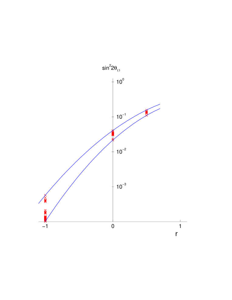
Figure 5: The prediction of $\sin^{2}2\theta_{13}$ as a function of the ratio of subdominant Yukawa couplings $r=a_{32}/a_{22}$ for the HSD class of models.

In Figure 3 we show results for HSD for $\tan\beta=50$, and $r=a_{32}/a_{22}=-1$. The results show a large rate for $\tau\rightarrow\mu\gamma$ which is the characteristic expectation of lop-sided models in general ^?) and HSD in particular. We also show the error incurred if the LLA were used (our results are based on an exact calculation). In Figure 4 we show results for LSD for $\tan\beta=50$, and $r=a_{32}/a_{22}=-1$. The results show a much smaller rate for $\tau\rightarrow\mu\gamma$, and also the error incurred if the LLA were used (our results are based on an exact calculation). In Figure 5 we show that the 13 mixing angle is controlled by a ratio of subdominant Yukawa couplings, $r=a_{32}/a_{22}$ and therefore cannot be predicted in general, although in particular models this ratio may be fixed by the theory.

8 LEPTOGENESIS AND ITS POSSIBLE RELATION TO CP VIOLATION MEASURED IN FUTURE NEUTRINO OSCILLATION EXPERIMENTS

Is there a link between the CP violation required for leptogenesis, and the phase $\delta$ measurable in accurate neutrino oscillation experiments? In general the answer would seem to be no, however in certain classes of models the answer can be yes. For example in sequential dominance we find that for HSD there is no link since the lightest right-handed neutrino of mass $X^{\prime}$ is quite relevant for leptogenesis, but completely irrelevant for the determining the neutrino angles and phases. However, in LSD there may be a link since in this case the lightest right-handed neutrino is also the dominant one, and so plays an important part in both leptogenesis and in determining the neutrino mixings and phases. Moreover in LSD the heaviest right-handed neutrino of mass $X^{\prime}$ is irrelevant for both leptogenesis and neutrino mixings and phases, so the model effectively reduces to a two right-handed neutrino model ^?).

The details of this have been recently worked out for the LSD class of models in which the neutrino matrices are as in Eqs.42,43 assuming the sequential dominance condition in Eq.25, and in addition assuming that $d=0$ which corresponds in this case to a 11 texture zero ^?). Although the class of model looks quite specialised, it is in fact extremely well motivated since it allows the neutrino Yukawa matrix to have the same universal form as the quark Yukawa matrices consistent with $SO(10)$ for example, where the 11 texture zero arises naturally ^?).

Returning to Eq.37, it may be expressed as

$$\tan\phi_{\rm COSMO}\approx\frac{|b|s_{23}s_{2}+|c|c_{23}s_{3}}{|b|s_{23}c_{2}+|c|c_{23}c_{3}}.$$ (63)

Inserting $\tilde{\phi}$ in Eq.36 into Eqs.34,35,

$$c_{23}|b|\sin(\eta_{2}+\phi_{\rm COSMO}+\delta)$$ (64)

$$\approx s_{23}|c|\sin(\eta_{3}+\phi_{\rm COSMO}+\delta).$$

Eq.64 may be expressed as

$$\tan(\phi_{\rm COSMO}+\delta)\approx\frac{|b|c_{23}s_{2}-|c|s_{23}s_{3}}{-|b|c_{23}c_{2}+|c|s_{23}c_{3}}$$ (65)

where we have written $s_{i}=\sin\eta_{i},c_{i}=\cos\eta_{i}$ where

$$\eta_{2}\equiv\phi_{b}-\phi_{e},\ \ \eta_{3}\equiv\phi_{c}-\phi_{f}$$ (66)

are invariant under a charged lepton phase transformation. The reason that the see-saw parameters only involve two invariant phases $\eta_{2},\eta_{3}$ rather than the usual six is due to the LSD assumption which has the effect of decoupling the heaviest right-handed neutrino, which removes three phases, together with the assumption of a 11 texture zero, which removes another phase.

Eq.65 shows that $\delta$ is a function of the two see-saw phases $\eta_{2},\eta_{3}$ that also determine $\phi_{\rm COSMO}$ in Eq.63. If both the phases $\eta_{2},\eta_{3}$ are zero, then both $\phi_{\rm COSMO}$ and $\delta$ are necessarily zero. This feature is absolutely crucial. It means that, barring cancellations, measurement of a non-zero value for the phase $\delta$ at a neutrino factory will be a signal of a non-zero value of the leptogenesis phase $\phi_{\rm COSMO}$. We also find the remarkable result

$$|\phi_{\rm COSMO}|=|\phi_{\beta\beta 0\nu}|.$$ (67)

where $\phi_{\beta\beta 0\nu}$ is the phase which enters the rate for neutrinoless double beta decay ^?).

To conclude, we have discussed the relation between leptogenesis and the MNS phases in the LSD class of models defined by Eqs.42,43,25 with the additional assumption of a 11 texture zero. Although the class of model looks quite specialised, it is in fact extremely well motivated since it allows the neutrino Yukawa matrix to have the same universal form as the quark Yukawa matrices consistent with $SO(10)$ for example, where the 11 texture zero arises naturally ^?). The large neutrino mixing angles and neutrino mass hierarchy then originate naturally from the sequential dominance mechanism without any fine tuning ^?). Within this class of models we have shown that the two see-saw phases $\eta_{2}$, $\eta_{3}$ are related to $\delta$ and $\phi_{\rm COSMO}$ according to Eqs.63,65. Remarkably, the leptogenesis phase is predicted to be equal to the neutrinoless double beta decay phase as in Eq.67. Since the heaviest right-handed neutrino of mass $X^{\prime}$ is irrelevant for both leptogenesis and for determining the neutrino masses and mixings, the model reduces effectively to one involving only two right-handed neutrinos ^?).

In this talk I have demonstrated that the physics of neutrino mass, flavour and CP violation are all closely linked. When the information from the neutrino sector is combined with that from the quark sector, including ideas of family symmetry and unification ^?), it is just possible that it may be enough to unlock the whole mystery of flavour.

9 Acknowledgements

I would like to thank Milla Baldo Ceolin for her kind hospitality at the X International Workshop on ”Neutrino Telescopes”.

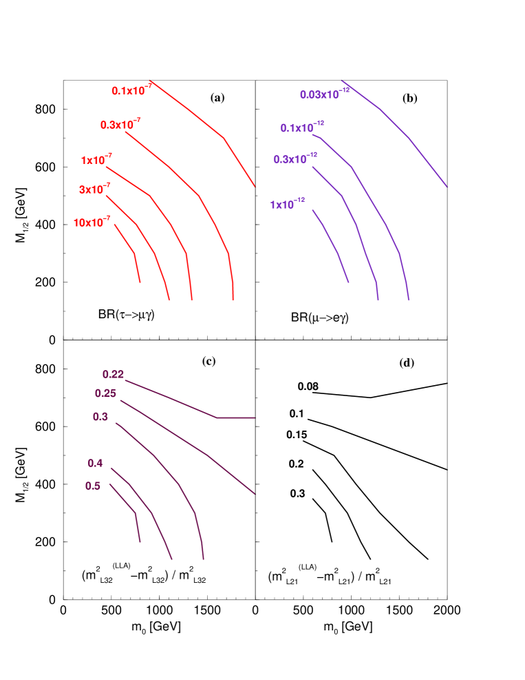
Figure 3: The upper panels show the predictions for the branching fraction for (a) $\tau\rightarrow\mu\gamma$ and (b) $\mu\rightarrow e\gamma$ for HSD using the parameters described in the text. The lower panels (c), (d) show the fractional error $\Delta_{ij}$, defined in the text, that would be made in calculating the off-diagonal slepton masses if the leading log approximation had been used instead of the exact calculation.

References

- [1] J.N. Bahcall, these proceedings.
- [2] A. Smirnov, these proceedings.
- [3] A. McDonald, these proceedings.
- [4] A. Suzuki, these proceedings.
- [5] T. Kajita, these proceedings.
- [6] Y. Suzuki, these proceedings.
- [7] G.L.Fogli, these proceedings.
- [8] L. Radicati di Brozolo,”The Bruno Pontecorvo Legacy”, these proceedings.
- [9] Z. Maki, M. Nakagawa and S. Sakata, Prog. Theor. Phys. 28 (1962) 870.
- [10] B. W. Lee, S. Pakvasa, R. E. Shrock and H. Sugawara, Phys. Rev. Lett. 38 (1977) 937 [Erratum-ibid. 38 (1977) 1230].
- [11] O. Elgaroy et al., galaxy redshift survey,” arXiv:astro-ph/0204152.
- [12] A. Pierce and H. Murayama, arXiv:hep-ph/0302131.
- [13] S. F. King, JHEP 0209 (2002) 011 [arXiv:hep-ph/0204360].
- [14] S. F. King and N. N. Singh, Nucl. Phys. B 596 (2001) 81 [arXiv:hep-ph/0007243].
- [15] R. Barbieri, L. J. Hall, D. R. Smith, A. Strumia and N. Weiner, JHEP 9812 (1998) 017 [arXiv:hep-ph/9807235].
- [16] S. Pascoli and S. T. Petcov, arXiv:hep-ph/0205022.
- [17] H. V. Klapdor-Kleingrothaus, A. Dietz, H. L. Harney and I. V. Krivosheina, Mod. Phys. Lett. A 16 (2001) 2409 [arXiv:hep-ph/0201231].
- [18] F. Feruglio, A. Strumia and F. Vissani, arXiv:hep-ph/0201291.
- [19] C. E. Aalseth et al., arXiv:hep-ex/0202018.
- [20] H. V. Klapdor-Kleingrothaus, arXiv:hep-ph/0205228.
- [21] S. Petcov, these proceedings.
- [22] K. Peach, these proceedings.
- [23] C. Weinheimer, these proceedings.
- [24] S. Choubey and S. F. King, Phys. Rev. D 67 (2003) 073005 [arXiv:hep-ph/0207260].
- [25] S. Glashow, these procedings.
- [26] S. F. King, Phys. Lett. B 439 (1998) 350 [arXiv:hep-ph/9806440].
- [27] S. F. King, Nucl. Phys. B 562 (1999) 57 [arXiv:hep-ph/9904210].
- [28] S. F. King, Nucl. Phys. B 576 (2000) 85 [arXiv:hep-ph/9912492].
- [29] S. F. King and N. N. Singh, Nucl. Phys. B 591 (2000) 3 [arXiv:hep-ph/0006229].
- [30] S. F. King and G. G. Ross, Phys. Lett. B 520 (2001) 243 [arXiv:hep-ph/0108112]; G. G. Ross and L.Velasco-Sevila, arXiv:hep-ph/0208218.
- [31] T. Blazek and S. F. King, arXiv:hep-ph/0211368.
- [32] T. Blazek and S. F. King, Phys. Lett. B 518 (2001) 109 [arXiv:hep-ph/0105005].
- [33] S. F. King, arXiv:hep-ph/0211228.