The $C$ parameter distribution in $e^{+}e^{-}$ annihilation

Abstract:

We study perturbative and non–perturbative aspects of the distribution of the $C$ parameter in $e^{+}e^{-}$ annihilation using renormalon techniques. We perform an exact calculation of the characteristic function, corresponding to the $C$ parameter differential cross section for a single off–shell gluon. We then concentrate on the two–jet region, derive the Borel representation of the Sudakov exponent in the large–$\beta_{0}$ limit and compare the result to that of the thrust $T$. Analysing the exponent, we distinguish two ingredients: the jet function, depending on $Q^{2}C$, summarizing the effects of collinear radiation, and a function describing soft emission at large angles, with momenta of order $QC$. The former is the same as for the thrust upon scaling $C$ by $1/6$, whereas the latter is different. We verify that the rescaled $C$ distribution coincides with that of $1-T$ to next–to–leading logarithmic accuracy, as predicted by Catani and Webber, and demonstrate that this relation breaks down beyond this order owing to soft radiation at large angles. The pattern of power corrections is also similar to that of the thrust: corrections appear as odd powers of $\Lambda/(QC)$. Based on the size of the renormalon ambiguity, however, the shape function is different: subleading power corrections for the $C$ distribution appear to be significantly smaller than those for the thrust.

1 Introduction

Event shape distributions have proven to be valuable in pushing forward our quantitative understanding of jet production and hadronization and of the interplay between perturbative and non–perturbative phenomena. Being infrared and collinear safe, these distributions can be computed order by order in perturbation theory, without the need to introduce non–perturbative parameters [1, 2, 3, 4, 5]. Even at large center–of–mass energies ($Q$), however, event–shape distributions involve substantial power corrections. As a consequence, they provide an important tool to study the onset of non–perturbative physics.

The two–jet region, where the distributions of most event shapes peak, is particularly important in this regard, and consequently it is also quite challenging. First of all, the perturbative analysis involves large Sudakov logarithms (double logarithms of the event shape $e$ which vanishes in the limit of two massless jets, examples being the $C$ parameter, jet masses $\rho_{J}$, and $t\equiv 1-T$, with $T$ the thrust). These logarithms make the perturbative coefficients of the distributions diverge at any finite order in the limit $e\to 0$. It is only upon resummation that one recovers the qualitative features of the cross section, namely the fact that it vanishes in the two–jet limit where radiation is inhibited (Sudakov suppression). A further complication is that power corrections, which are associated with large–angle soft emission, are also enhanced in this limit, as the relevant scale is typically $Qe$.

The resummation of large perturbative corrections [6, 7, 8, 9, 10, 11, 12, 13, 14, 15] and the parameterization of power corrections based on renormalon techniques [16, 17, 18, 19, 20, 21, 22, 23, 24, 25, 26, 27, 28, 29, 30, 31, 32, 33, 34, 35, 36, 37, 38] have opened up the way for quantitative predictions in the two–jet region. While much progress was made during the LEP era, some of the fundamental questions concerning power corrections have not yet been fully answered. A classical example is the relation (“universality”) between corrections to different observables which may be deduced from renormalon models. Even a more pragmatic motivation to study event shapes, namely to provide a precise measurement of the strong coupling, is hampered by theoretical uncertainties [39, 34, 36, 37]. Thus, in spite of having no active $e^{+}e^{-}$ collider, further theoretical progress is important. Progress is made nowadays in fixed–order calculations [40], as well as in resummation and parametrization of power corrections [42, 43, 41, 44, 45, 46]. Tools developed in the context of event shapes in $e^{+}e^{-}$ annihilation are often used in other applications.

One of the aspects where the study of event shapes has taught us general lessons about QCD is the interplay between perturbative and non–perturbative corrections. The phenomenological success of renormalon–based models for power corrections has important consequences. On the one hand, it shows that perturbative tools are quite powerful. In a sense, the state–of–the–art theoretical description of event–shape distributions pushes perturbative calculations beyond their natural regime of applicability. In general, this relies on the understanding that hadronization is a soft phenomenon, which does not involve significant momentum flow and thus does not change drastically the perturbative distribution. On the other hand, the success of these models implies that there is no way to quantify non–perturbative corrections and relate them to matrix elements without controlling first perturbative corrections to all orders. This stands in sharp contrast to the standard approach taken when vacuum condensates are estimated in the framework of QCD sum rules [47]. The current understanding of power corrections highlights the significance of running–coupling effects at the perturbative level.

Our main focus in this paper is the two–jet region. Quantitative predictions in this region are highly non–trivial, involving large logarithmic corrections from multiple soft and collinear gluon radiation, as well as significant running–coupling effects. The latter have both perturbative and non–perturbative aspects, and some of the difficulty is related to the ambiguous separation between them. An important feature of the two–jet region is the fact that, as $e\to 0$, it becomes necessary to resum not only singular perturbative contributions, but power corrections as well: in fact for values of $e={\cal O}(\Lambda/Q)$, which are not far from the peak of the distribution in typical LEP data, all power corrections of the form $(\Lambda/(Qe))^{p}$ become equally important. The feasibility in principle of such a resummation was shown in Refs. [21, 22], extending the factorization of the cross section in the two–jet limit to power–suppressed effects. Power corrections of this kind can be summarized in a “shape function”, which can be naturally combined with the effects of Sudakov resummation. Renormalon calculations can then be used to construct highly constrained QCD models for the shape function. In this paper, we will essentially construct such a model for the $C$ parameter distribution, following the Dressed Gluon Exponentiation (DGE) approach, first developed in connection with the thrust distribution [36]. In this approach one computes and resums Sudakov logs and renormalons simultaneously, obtaining information on leading as well as subleading power corrections, which can be summarized if desired in an ansatz for the shape function. Note that the combination of Sudakov effects with parametrically enhanced power corrections is definitely not unique to event–shape distributions. It appears whenever differential cross sections in QCD are evaluated near a kinematic threshold; other important examples are Drell–Yan production near the energy threshold [19, 32], structure functions near the elastic limit (Bjorken $x$ close to $1$) [48, 49], and fragmentation functions of light [30, 38] and heavy quarks [50] near $z=1$. In spite of the different nature of these processes, certain characteristics of the perturbative expansion are generic [38], and similar techniques are applicable in all cases.

As announced, we will consider here the distribution of a specific event–shape variable, the $C$ parameter. This variable was first proposed 25 years ago [2], and became one of the classical examples of infrared and collinear safe observables. A next–to–leading order (NLO) ${\cal O}(\alpha_{s}^{2})$ calculation for the distribution of the $C$ parameter was performed long ago[5] (the next order is still not available), while the resummation of Sudakov logs to next–to–leading logarithmic accuracy (NLL) has become available only recently [13]. In the last few years the example of the $C$ parameter, and in particular its average value, had an important place in the ongoing debate concerning universality of power corrections, see e.g. [13, 23, 30, 31]. On the other hand, as far as the resummation of running–coupling effects is concerned, the $C$ parameter distribution was not analysed, and the prime example has always been the thrust [34, 35].

The study of the thrust and of the heavy–jet mass distributions by means of DGE [36, 37] highlighted several significant features of higher–order perturbative as well as non–perturbative contributions. In particular, it was found that subleading Sudakov logs, that are usually neglected, can give substantial contributions: they carry the factorial enhancement of renormalons. Phenomenologically, the refinement of the calculated distribution by DGE (as compared to the standard resummation to NLL accuracy) turned out to have a dramatic effect on data fits in the peak region. The most impressive demonstration of this fact is the agreement between the non–perturbative parameters extracted from the thrust and the heavy–jet mass distributions [37]. The effect this resummation has on the extracted value of the coupling is also substantial. It is, of course, of great interest to extend the DGE analysis to other event–shape variables and learn which features are generic and which depend on the observable. The purpose of this paper is to perform such an analysis for the $C$ parameter.

We proceed as follows. In the next section we recall the definition of the $C$ parameter, present the kinematics in a three–particle final state where the gluon is off shell, and compute the characteristic function. The final result is summarized in Appendix A. In Section 3 we expand the characteristic function at small $C$ (details are given in Appendix B) in order to identify the source of logarithmically enhanced terms which dominate the two–jet limit; next, we construct a Borel representation of the Sudakov exponent, and we use it to extract perturbative as well as non–perturbative information on the distribution, comparing it with the case of the thrust. Our results are summarized and briefly discussed in Section 4.

2 The characteristic function

The $C$ parameter for electron–positron annihilation events was originally defined [3, 4] as

$$C=3(\lambda_{1}\lambda_{2}+\lambda_{2}\lambda_{3}+\lambda_{3}\lambda_{1})~{},$$ (1)

where $\lambda_{\alpha}$ are the eigenvalues of the matrix

$$\Theta_{\alpha\beta}=\frac{1}{\sum_{j}\left|{\bf p}^{(j)}\right|}\,\sum_{i}\frac{{\bf p}_{\alpha}^{(i)}\,{\bf p}_{\beta}^{(i)}}{\left|{\bf p}^{(i)}\right|}~{},$$ (2)

and ${\bf p}_{\alpha}^{(i)}$ are the spatial components ($\alpha=1,2,3$) of the $i$–th particle momentum in the center–of–mass frame. The sums over $i$ and $j$ run over all the final state particles.

A related definition in terms of Lorentz invariants is

$$C=3-\frac{3}{2}\sum_{i,j}\frac{(p^{(i)}\cdot p^{(j)})^{2}}{(p^{(i)}\cdot q)\,(p^{(j)}\cdot q)}~{},$$ (3)

where $p^{(i)}$ is the four–momentum of the $i$–th particle and $q$ is the total four momentum, $q=\sum_{i}p^{(i)}$. The two definitions are equivalent provided particle masses are neglected (for a discussion of mass effects in power corrections, see [51]).

The $C$ parameter varies in the range $0\leq C\leq 1$. $C=0$ corresponds to a perfect two–jet event (with massless jets), while $C=1$ characterizes a spherical event. Planar events, including, in particular, the ${\cal O}(\alpha_{s})$ perturbative result, are distributed in the range $0\leq C\leq 3/4$.

The information needed to perform renormalon resummation at the level of a single dressed gluon (the large–$\beta_{0}$ limit) and, eventually, learn about power corrections, is present in the leading–order differential cross section, calculated with an off–shell gluon [16, 27, 52], sometimes called “characteristic function”. In this section we present an exact calculation of the characteristic function for the distribution of the $C$ parameter. An analogous calculation for the thrust was performed in [35]. Although the calculation and the general structure of the result are similar, in the case under consideration the expressions involved are significantly more complicated.

It should be noted that the renormalon calculation we perform treats the decay of the gluon inclusively. The characteristic function depends only on the total invariant mass of the particles eventually produced by the gluon and not on their separate momenta. Since event–shape variables such as the $C$ parameter are sensitive to the momenta of individual final–state particles, our calculation differs, for example, from a strict large–$N_{f}$ limit. This point was first noted in [25], and was since addressed in various occasions, first in applications to single–particle inclusive cross sections [33], then in the context of the conjectured universality of power corrections [29]. In the thrust case the inclusive approximation is good, in the sense that higher–order perturbative terms are numerically close to the strict large–$N_{f}$ result [34, 35, 36] (larger differences occur if one considers purely non–Abelian contributions). The approximation is especially good in the two–jet limit in which we are interested. In the case of the average $C$ parameter, Smye [31] has performed a detailed analysis of the effect non–inclusive contributions have on the coefficient of the $1/Q$ correction, within the framework of [29]. Also in this case the inclusive approximation is close to the large–$N_{f}$ result, while larger differences appear in the non–Abelian part. An analysis of this kind has not yet been performed for the distribution. We observe also that it is unclear to what extent non–inclusive contributions can consistently be treated within the framework of the dispersive approach, since they contain terms that are genuinely unrelated to running–coupling effects, even in the abelian limit.

It should be kept in mind that, with present technology, renormalon models can only be used as a tool to gather information on the general structure of power corrections, and possibly a rough estimate on their size. For such purposes, we believe that the inclusive approximation is sufficient, a view which is supported by the phenomenological success of the data fits performed with it, and also by the small relative size of the non–inclusive correction in the cases in which it was computed. Given the complexity of the calculation in the case of the $C$ parameter, we will not attempt here a calculation in the strict large–$N_{f}$ limit. A calculation of the distribution along the lines of [31] would in any case be welcome, since it would improve the control on phase–space effects, and gauge the stability of our result.

In order to perform the calculation of the characteristic function we first calculate the $C$ parameter for a three–particle final state: a quark and an antiquark with momenta $p_{1}$ and $p_{2}$ ($p_{1}^{2}=p_{2}^{2}=0$) and an off–shell gluon with momentum $k$. It is convenient to define the normalized gluon virtuality by $\xi\equiv k^{2}/q^{2}$, and the variables

$$x_{1} = 2p_{1}\cdot q/q^{2}~{},$$

$$x_{2} = 2p_{2}\cdot q/q^{2}~{},$$ (4)

$$y = 2k\cdot q/q^{2}\,=\,2-x_{1}-x_{2}~{},$$

which correspond to the energy fractions in the centre–of–mass frame. Using these variables one finds

$${\bf c}(x_{1},x_{2},\xi)\,\equiv\,C/6\,=\,\frac{(1-x_{1})(1-x_{2})(1-y+2\xi)-\xi^{2}}{x_{1}x_{2}y}~{}.$$ (5)

Here we rescaled the shape variable by a factor of 6; we will compute the differential cross section for the rescaled variable $c$, from which the standard observable can be readily obtained, as

$$\frac{1}{\sigma}\frac{d\sigma}{dC}(C,Q^{2})=\frac{1}{6}\left.\frac{1}{\sigma}\frac{d\sigma}{dc}(c,Q^{2})\right|_{c=C/6}~{}.$$ (6)

Depending on the precise interpretation of the definition of the $C$ parameter for massive particles there can be in Eq. (5) an additional term (from $i$ and $j$ in (3) both corresponding to the gluon) of the form $-\xi^{2}/y^{2}$. Here, however, we will be using Eq. (5) as written. As we shall see below, in the small–$c$ region, $c={\cal O}(\xi/y)$, so this term is negligible.

The renormalon–resummed differential cross section in the single dressed gluon approximation is

$$\frac{1}{\sigma}\frac{d\sigma}{dc}(c,Q^{2})=-\frac{C_{F}}{2\beta_{0}}\,\int_{0}^{1}{d\xi}\,\frac{d{\cal F}(\xi,c)}{d\xi}\,A(\xi Q^{2})~{},$$ (7)

where $\beta_{0}=\frac{11}{12}C_{A}-\frac{1}{6}N_{f}$, and $A(\xi Q^{2})$ is the large–$\beta_{0}$ running coupling ($A=\beta_{0}\alpha_{s}/\pi$) on the time–like axis, admitting the Borel representation

$$A(\xi Q^{2})=\int_{0}^{\infty}du\,\left(Q^{2}/\Lambda^{2}\right)^{-u}\,\frac{\sin\pi u}{\pi u}\,{\rm e}^{\frac{5}{3}u}\,\xi^{-u}\,,$$ (8)

where $\Lambda$ is the QCD scale in the ${\overline{\rm MS}}$ scheme, the constant $5/3$ comes from the renormalization of the fermion loop in this scheme, and the sine factor originates in the analytic continuation to the time–like axis.

The characteristic function is of the form

$${\cal F}(\xi,c)=\int dx_{1}dx_{2}\,{\cal M}(x_{1},x_{2},\xi)\,\delta\left({\bf c}(x_{1},x_{2},\xi)-c\right)~{}.$$ (9)

Here ${\cal M}$ is the squared matrix element for $\gamma^{*}\longrightarrow q\overline{q}g$ (with the coupling and the colour factor extracted), and is given by

$${\cal M}(x_{1},x_{2},\xi)=\frac{(x_{1}+\xi)^{2}+(x_{2}+\xi)^{2}}{(1-x_{1})(1-x_{2})}-\frac{\xi}{(1-x_{1})^{2}}-\frac{\xi}{(1-x_{2})^{2}}~{}.$$ (10)

Phase space (illustrated in figure 1) is limited by the restrictions

$${\rm hard\,limit} x_{1}+x_{2}\geq 1-\xi~{},$$

$${\rm soft\,limit} (1-x_{1})(1-x_{2})\geq\xi~{},$$ (11)

where the hard and soft limits correspond to the upper and lower bounds on the gluon energy fraction $y=2-x_{1}-x_{2}$.

Note that along the soft limit, which will be our main interest in the next section, the expression for $c$ in Eq. (5) simplifies a lot. One gets

$$\left.{\bf c}(x_{1},x_{2},\xi)\right|_{\rm soft}=\xi/y~{}.$$ (12)

Along this phase–space boundary, the maximal value for $c$ with fixed $\xi$ is obtained for $x_{1}=x_{2}=1-\sqrt{\xi}$, so $y=y_{\min}=2\sqrt{\xi}$ and $c_{\max}^{{\rm soft}}=\sqrt{\xi}/2$. This is the relevant phase–space limit for large–angle soft gluon emission. The minimal value of $c$ is obtained in the intersection with the hard limit, for either $x_{1}=0$ or $x_{2}=0$, so $y=y_{\max}=1+\xi$ and $c_{\min}=\xi/(1+\xi)$. This is the relevant limit for collinear gluon emission. The maximum value of $c$ is attained away from the boundaries of phase space, as seen in Figure 1. It can be determined by maximizing the explicit expression in Eq. (5) within the physical region, and for small $\xi$ is given by $c_{\max}=1/8+3\xi/4+{\cal O}(\xi^{2})$.

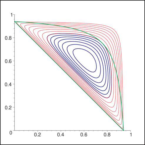
Figure 1: The $x_{1}$ – $x_{2}$ plane for a fixed $\xi=0.06$. The phase–space limits (2) (green) are shown together with contours of fixed $c$ belonging to the two regions in (21): contours that close within the phase–space boundaries, corresponding to $F_{h}$ (thick, blue), and contours that reach the soft phase–space limit, corresponding to $F_{l}$ (thin, red).

In order to perform the integrations in (9), it is convenient to change variables from $x_{1}$ and $x_{2}$ into $y$ and $z=(1-x_{2})/y$. In the new variables the integral has the form

$${\cal F}(\xi,c) = \int_{2\sqrt{\xi}}^{1+\xi}\frac{dy}{y}\int_{\frac{1}{2}\left(1-\sqrt{1-4\xi/y^{2}}\right)}^{\frac{1}{2}\left(1+\sqrt{1-4\xi/y^{2}}\right)}dz\,\delta\left((z-z_{+})(z-z_{-})\frac{y(1+2\xi-y(1+c))}{(1-yz)(1-y(1-z))}\right)$$ (13)

$$\,\left[\frac{(1-y(1-z))^{2}+(1-yz)^{2}+2\xi(2+\xi-y)}{z(1-z)}-\frac{\xi}{z^{2}}-\frac{\xi}{(1-z)^{2}}\right]\,,$$

where

$$z_{\pm}=\frac{1}{2}\left[1\pm\sqrt{1-\frac{4(cy(1-y)+\xi^{2})}{y^{2}(1+2\xi-y(1+c))}}\right]\,.$$ (14)

Here the symmetry $x_{1}\longleftrightarrow x_{2}$ appears as $z\longleftrightarrow 1-z$. Using this symmetry, the integral over $z$ equals twice the integral between the lower limit in Eq. (13) and $z=1/2$, where only $z=z_{-}$ in the $\delta$ function is relevant. The condition $z_{-}\geq{\frac{1}{2}\left(1-\sqrt{1-4\xi/y^{2}}\right)}$ for physical values of $c$ implies that

$$\frac{\xi}{c}\,\leq\,y\,\leq\,\frac{1+2\xi}{1+c}\equiv y_{0}\,.$$ (15)

The condition that $z_{-}$ be real, on the other hand, implies that

$$(1+c)y^{3}-(1+2\xi+4c)y^{2}+4cy+4\xi^{2}\leq 0\,.$$ (16)

It turns out that within the physical region all three roots $y_{1,2,3}$ of Eq. (16) are real. Choosing $y_{1}\leq y_{2}\leq y_{3}$, Eq. (16) requires that

$$y_{2}\leq y\leq y_{3}~{}.$$ (17)

Investigating the solutions of Eq. (16), one finds that $y_{2}>{\xi}/c$ for $c>\sqrt{\xi}/2$, while $y_{2}\leq{\xi}/c$ for $c\leq\sqrt{\xi}/2$, so the conditions (17) and (15) together imply that the lower integration limit over $y$ is $y_{2}$ for $c>\sqrt{\xi}/2$, but it is $\xi/c$ for $c\leq\sqrt{\xi}/2$. The result is therefore

$${\cal F}(\xi,c) = \left\{\begin{array}[]{ll}\displaystyle{{\cal F}_{l}(\xi,c)\equiv\int_{\xi/c}^{y_{3}}dyf(y,c,\xi)}&\hskip 40.0pt\frac{\xi}{1+\xi}\,\leq\,c\,\leq\,\frac{\sqrt{\xi}}{2}~{},\\ \\ {\cal F}_{h}(\xi,c)\equiv\displaystyle{\int_{y_{2}}^{y_{3}}dyf(y,c,\xi)}&\hskip 40.0pt\frac{\sqrt{\xi}}{2}\,<\,c\,\leq\,c_{\max}=\frac{1}{8}+\frac{3}{4}\xi+{\cal O}(\xi^{2})~{},\end{array}\right.$$ (21)

where

$$f(y,c,\xi) = \frac{2}{(1+c)^{2}}\frac{y(1+\xi-y)^{3}}{(cy(1-y)+\xi^{2})^{2}\,\sqrt{(y_{0}-y)^{3}(y_{3}-y)(y-y_{1})(y-y_{2})}}$$

$$\times\Big{[}-c\,(1+c)\,y^{4}+((5\,c+2\,c^{2}+1)\,\xi+3\,c+4\,c^{2})\,y^{3}$$

$$\,\,\,\,\,\,+((-2-4\,c)\,\xi^{2}+(-2\,c^{2}-1-10\,c)\,\xi-4\,c-4\,c^{2})\,y^{2}$$

$$\,\,\,\,\,\,+((-2\,c-2)\,\xi^{3}-2\,\xi^{2}+8\,\xi\,c+2\,c)\,y+4\,\xi^{4}+8\,\xi^{3}+2\,\xi^{2}\Big{]}\,.$$

The two regions of the parameter space of Eq. (21) are distinguished by whether, for fixed $\xi$ and $c$, the soft phase–space limit in Eq. (2) can be reached. The corresponding classes of contours are shown in Figure 1 in the $x_{1}$ – $x_{2}$ plane. A similar situation occurs in the case of the thrust distribution [35]. In both cases the characteristic function is given by two different analytic function in these two regions.

Finally, ${\cal F}(\xi,c)$ can be expressed as a sum of standard elliptic integrals. These are complete elliptic integrals for ${\cal F}_{h}(\xi,c)$ and incomplete ones for ${\cal F}_{l}(\xi,c)$. The explicit expressions are given in Appendix A.

3 The Sudakov exponent

Having calculated the characteristic function for the distribution of the $C$ parameter, we can use DGE to compute the Sudakov exponent for the two–jet limit in the large–$\beta_{0}$ limit. The procedure we follow was introduced in [36], where the exponent for the thrust distribution was computed. Similar calculations were done since for heavy–jet mass distribution [37], light–quark fragmentation, deep inelastic structure functions and Drell–Yan production for $x\longrightarrow 1$ [38], and, most recently, the heavy–quark fragmentation function [50].

The Borel representation of Eq. (7) can be constructed by using the explicit expression for $A(\xi Q^{2})$ given in Eq. (8) and changing the order of integration. One obtains

$$\left.\frac{1}{\sigma}\frac{d\sigma}{dc}(c,Q^{2})\right|_{\hbox{\tiny SDG}}=\frac{C_{F}}{2\beta_{0}}\,\int_{0}^{\infty}du\,\left(Q^{2}/\Lambda^{2}\right)^{-u}\,B(c,u)\,,$$ (23)

where the subscript stands for a Single Dressed Gluon. The Borel function is

$$B(c,u)\,=\,-\,\frac{\sin\pi u}{\pi u}\,{\rm e}^{\frac{5}{3}u}\,\left[\int_{0}^{4c^{2}}{d\xi}\,\frac{d{\cal F}_{h}(\xi,c)}{d\xi}\,\xi^{-u}\,+\,\int_{4c^{2}}^{c/(1-c)}{d\xi}\,\frac{d{\cal F}_{l}(\xi,c)}{d\xi}\,\xi^{-u}\right]\,.$$ (24)

While these expressions are completely general, and can be used to resum the renormalons in the large–$\beta_{0}$ limit for arbitrary $c$, we are interested specifically in Sudakov logs, which dominate the cross section in the two–jet region. Starting from the full characteristic function, the first step is to identify the ${\cal O}(1/c)$ singular terms, namely those terms that upon integration over the gluon virtuality in Eq. (7) or in Eq. (24) would lead to logarithmically enhanced contributions in the perturbative expansion of the distribution.

The identification of the relevant terms was straightforward in the case of the thrust, but it is much less so here, given the complexity of the characteristic function, Eq. (21). One can expand the integrand given in Eq. (2) or the closed–form expressions of Appendix A at small $c$, but this requires of course to specify how $\xi$ behaves in the limit considered. Given the limits of integration in Eq. (24), there are two natural $c\to 0$ limits to consider: one with fixed $a\equiv\xi/c$, which is relevant in the collinear region, and the second with fixed $b\equiv\xi/c^{2}$, relevant in the large–angle soft emission region.

On general grounds, one expects Sudakov logs to emerge from the soft boundary of phase space in Eq. (2). Figure 1 shows that only for ${\cal F}_{l}$ the soft boundary of phase space is relevant, so it is only the second term in Eq. (24) that is expected to be relevant. We will verify this statement explicitly below. A similar situation occurs for the thrust distribution [36].

The details of the small–$c$ expansion of ${\cal F}_{l}$ at fixed $a$ and at fixed $b$, and of ${\cal F}_{h}$ at fixed $b$, are summarized in Appendix B. The final results for the leading ${\cal O}(1/c)$ terms are

$$\left.{\cal F}_{l}(\xi,c)\right|_{{\rm fixed}\,a\equiv\xi/c} = \frac{1}{c}\left[-4\ln a-3+2a+a^{2}\right]+{\cal O}(c^{0})$$

$$\left.{\cal F}_{l}(\xi,c)\right|_{{\rm fixed}\,b\equiv\xi/c^{2}} = \frac{1}{c}\left[-4\ln bc-3-8\ln\left(\frac{1}{2}\left(1+\sqrt{1-4/b}\right)\right)\right]+{\cal O}(c^{0})\,,$$ (25)

while

$$\left.{\cal F}_{h}(\xi,c)\right|_{{\rm fixed}\,b\equiv\xi/c^{2}}=\frac{1}{c}\left[-4\ln c-3\right]+{\cal O}(c^{0})\,.$$ (26)

Eq. (26)) implies that indeed the first term in Eq. (24), the one involving ${\cal F}_{h}$, is irrelevant for logarithmically enhanced terms. In order to compute the Sudakov exponent we therefore concentrate on $F_{l}$. Using Eq. (3) it is straightforward to write down an expression for $F_{l}$ that has the correct ${\cal O}(1/c)$ terms both for fixed $a$ and for fixed $b$. It is given by

$$\left.{\cal F}_{l}(\xi,c)\right|_{{\cal O}(1/c)}\!=\!\frac{1}{c}\left[-4\ln\left(\frac{\xi}{c}\right)-3+2\left(\frac{\xi}{c}\right)+\left(\frac{\xi}{c}\right)^{2}-8\ln\left(\frac{1}{2}\left(1+\sqrt{1-4c^{2}/\xi}\right)\right)\right].$$ (27)

Taking a derivative of Eq. (27) and substituting into Eq. (24) we find

$$\left.B(c,u)\right|_{\rm logs}\,=\,2{\rm e}^{\frac{5}{3}u}\,\frac{\sin\pi u}{\pi u}\,\int_{4c^{2}}^{c}{d\xi}\,\xi^{-u}\left[\frac{2}{\xi c}-\frac{1}{c^{2}}-\frac{\xi}{c^{3}}+\frac{8c}{\xi\sqrt{\xi-4c^{2}}\left(\sqrt{\xi}+\sqrt{\xi-4c^{2}}\right)}\right]\,,$$ (28)

where we simplified the upper limit without affecting the relevant (log–enhanced) terms. As expected from Eq. (3), only the first and the last terms in the square brackets in Eq. (28) contribute to the Sudakov exponent owing to the lower (large–angle) integration limit, while the first three terms, and not the last, contribute owing to the upper (collinear) limit. The result of the integration is

$$\left.B(c,u)\right|_{\rm logs}\,=\,2{\rm e}^{\frac{5}{3}u}\,\frac{\sin\pi u}{\pi u}\,\left[4(2c)^{-1-2u}\frac{\sqrt{\pi}\Gamma(u)}{\Gamma(\frac{1}{2}+u)}-c^{-1-u}\left(\frac{2}{u}+\frac{1}{1-u}+\frac{1}{2-u}\right)\right]\,.$$ (29)

This simple expression summarizes all log–enhanced contributions to the $c$ distribution (23), to any order in perturbation theory, in the large–$\beta_{0}$ limit. The result is written as a sum of two ingredients, each originating in a different region of phase space: the first, where the relevant scale is $4Q^{2}c^{2}$ (gluon virtuality $\xi\simeq 4c^{2}$) is associated with large–angle soft emission (it can be traced through the calculation to the region where $y\simeq 2\sqrt{\xi}$ and $x_{1}\simeq x_{2}\simeq 1-\sqrt{\xi}$); the second, where the scale is $Q^{2}c$ (gluon virtuality $\xi\simeq c$) is associated with collinear emission (corresponding to $y\simeq 1+\xi$, and either $x_{1}\simeq 0$ or $x_{2}\simeq 0$). Note that infrared safety is guaranteed in Eq. (29) thanks to the cancellation between ${\cal O}(1/u)$ terms between the soft and the collinear ingredients, so each of these ingredients is ill–defined unless a factorization prescription is introduced. Note also that Eq. (29) is free of renormalon singularities, but the Borel integral (23) does have convergence constraints at small $c$, which will turn into renormalons in the Sudakov exponent upon performing the necessary Laplace transform, as outlined below.

For comparison we quote the analogous result for the thrust distribution [36, 38]. Defining $t=1-T$, the Borel function in the large–$\beta_{0}$ limit is

$$\left.B(t,u)\right|_{\rm logs}\,=\,2{\rm e}^{\frac{5}{3}u}\,\frac{\sin\pi u}{\pi u}\,\left[\frac{2}{u}\,t^{-1-2u}-t^{-1-u}\left(\frac{2}{u}+\frac{1}{1-u}+\frac{1}{2-u}\right)\right]\,.$$ (30)

The result for the heavy–jet mass [37] (in this approximation) is the same as Eq. (30) up to an overall factor of $1/2$. The similarity, as well as the differences, between Eq. (29) and Eq. (30) are easily understood: the collinear ingredient is identical (with $c$ replaced by $t$), while the large–angle soft emission ingredient is different. In fact, replacing $c$ by $1-x$, the collinear ingredient coincides with the large–$\beta_{0}$ expression [38] for the jet function [7, 8, 9] which controls the large–$x$ limit in single–particle inclusive cross–sections in $e^{+}e^{-}$ annihilation [38, 50], as well as for structure functions near the elastic limit [48, 49]. This object describes the radiation from an unobserved jet under a restriction on its invariant mass. It therefore appears in each of these observables.

As noted above, the large–angle soft emission ingredient for the $c$ distribution in Eq. (29) turns out to be quite different from that of the thrust, in Eq. (30). This is not surprising: different event–shape variables weigh differently the soft radiation. One immediately recognizes that the relevant scale of large–angle soft radiation in the $c$ distribution is $2Qc$, while for thrust it is $Qt$. As we shall see below this factor of $2$ suppresses subleading logarithmic corrections, as well as subleading power corrections, in the case of $c$, as compared to $t$.

We now turn to the computation of the Sudakov exponent. Owing to the additivity property of the $C$ parameter in the small $C$ limit with respect to multiple emission, and the factorization property of QCD matrix elements for soft and collinear radiation, logarithmically enhanced terms in the perturbative expansion exponentiate in Laplace space. Consequently, the resummed cross section can be written, in full analogy with the thrust [10, 36], as

$$\left.\frac{1}{\sigma}\frac{d\sigma}{dc}(c,Q^{2})\right|_{\hbox{\tiny DGE}}=\int_{k-{\rm i}\infty}^{k+{\rm i}\infty}\frac{d\nu}{2\pi{\rm i}}\,{\rm e}^{\nu c}\,\exp\left[S(\nu,Q^{2})\right]\,,$$ (31)

where $k$ is to the right of the singularities of the integrand. The Sudakov exponent is given by

$$S(\nu,Q^{2})\equiv\left<e^{-\nu c}\right>=\int_{0}^{\infty}\,d\tilde{c}\,\left.\frac{1}{\sigma}\frac{d\sigma}{d{\tilde{c}}}(\tilde{c},Q^{2})\right|_{\hbox{\tiny SDG}}\left({\rm e}^{-\nu\tilde{c}}-1\right)\,,$$ (32)

where the upper limit of integration was extended to infinity (i.e. beyond the range where the physical distribution has support) to comply with the standard definition of the Laplace transform. The integral is dominated by the Sudakov region, so that singular terms for $c\to 0$ in Eq. (23) generate logarithmically divergent terms for $\nu\to\infty$ in $S(\nu,Q^{2})$. It should be noted that, as far as these singular terms are concerned, and to any logarithmic accuracy, the Laplace transform is equivalent to a Mellin transform, where $\nu$ is the moment conjugate to $1-\tilde{c}$.

Next, we compute $S(\nu,Q^{2})$ in the large–$\beta_{0}$ limit using Eq. (23) and Eq. (29). The result is

$$S(\nu,Q^{2})=\frac{C_{F}}{2\beta_{0}}\,\int_{0}^{\infty}du\,\left(Q^{2}/\Lambda^{2}\right)^{-u}\,B_{\nu}^{c}(u)\,,$$ (33)

with

$$B_{\nu}^{c}(u) = \int_{0}^{\infty}dc\,B(c,u)\,\left({\rm e}^{-\nu c}-1\right)=\,2{\rm e}^{\frac{5}{3}u}\,\frac{\sin\pi u}{\pi u}\,\left[\Gamma(-2u)\left(\nu^{2u}-1\right)2^{1-2u}\frac{\sqrt{\pi}\Gamma(u)}{\Gamma(\frac{1}{2}+u)}\right.$$ (34)

$$\hskip 80.0pt-\left.\Gamma(-u)\left({\nu}^{u}-1\right)\left(\frac{2}{u}+\frac{1}{1-u}+\frac{1}{2-u}\right)\right]\,,$$

where terms suppressed by powers of $1/\nu$ were neglected.

Contrary to Eq. (29), the Borel function in Laplace space given by Eq. (34) has renormalon singularities. The appearance of infrared renormalons as a consequence of taking a Laplace or a Mellin transform is characteristic of differential cross–sections near a kinematic threshold [36, 38, 49, 50]. In Eq. (34) renormalons appear in both the large–angle soft emission factor and in the jet function. In the former, they correspond to corrections that scale as odd powers of $Q/\nu$, while in the latter to ones that scale as the first two powers of $Q^{2}/\nu$, i.e. twist four and twist six, as in structure functions. The leading power corrections in the Sudakov region (so long as $Q^{2}c\gg\Lambda^{2}$) are of the former type, and they can be summed up into a shape function, as discussed in [19, 20, 21, 22, 23, 36, 37]. We further address this issue below.

Eq. (34), together with Eq. (33) and Eq. (31), is our final result for the $c$ distribution, calculated by DGE. The experience gained in the case of the thrust and the heavy–jet mass distributions [36, 37] shows that there is a significant difference between the resummed cross section à la DGE and standard resummation with NLL accuracy. Owing to the renormalon factorial growth, the additional terms (subleading logs) which are resummed by DGE and neglected otherwise are numerically important. DGE has a significant impact on the quality of the description of the distribution in the peak region, on the extracted non–perturbative parameters, and, in particular, on the consistency of the latter between the thrust and the heavy–jet mass distributions. It is therefore important to analyse more event–shape distributions with the same methodology, and the road is now open to do so for the $C$ parameter.

It should be emphasized that controlling the large–$\beta_{0}$ terms is sufficient for generating the entire set of logs up to NLL accuracy. This can be done [36] by promoting the running coupling of Eq. (8) to two loops, while replacing the constant $5/3$ in the exponent by the full coefficient of the $x\to 1$ singular term in the NLO splitting function [12], according to

$$\frac{5}{3}\,\longrightarrow\,\frac{5}{3}+\left(\frac{1}{3}-\frac{\pi^{2}}{12}\right)\frac{C_{A}}{\beta_{0}}\,.$$ (35)

One should keep in mind, though, that this replacement is sufficient only to NLL accuracy, while the correct generalization of the Borel function (34) beyond the large–$\beta_{0}$ limit is not known. See [49] for a relevant discussion.

Of course, as it stands, the integral in Eq. (33) is ill defined due to its renormalons singularities. It is straightforward, however, to perform a principal–value regularization either analytically [36, 37] or numerically [50]. The size of the ambiguity of Eq. (33), as measured by the residues of the singularities, can be used as an estimate of the size of the corresponding power corrections, as discussed below. Let us also recall that, in order to use the DGE result in practice, one needs to match it onto the known fixed–order calculation, to take into account terms which are not logarithmically enhanced. The procedure [36] is similar to the one used in a standard NLL resummation program [10].

The location of the renormalons in Eq. (34) is identical to the case of the thrust. For easy comparison we quote the analogous expression derived in that case, where $\nu$ is the Laplace conjugate variable to $t=1-T$. It is given by

$$B_{\nu}^{t}(u)=\,2{\rm e}^{\frac{5}{3}u}\,\frac{\sin\pi u}{\pi u}\left[\Gamma(-2u)\left(\nu^{2u}-1\right)\frac{2}{u}-\Gamma(-u)\left(\nu^{u}-1\right)\left(\frac{2}{u}+\frac{1}{1-u}+\frac{1}{2-u}\right)\right]\,.$$ (36)

In order to extract the perturbative coefficients of the exponent $S(\nu,Q^{2})$ in the large–$\beta_{0}$ limit, it is sufficient to expand $B_{\nu}(u)$ in powers of $u$ and replace $u^{n}$ by $n!\left(\beta_{0}\alpha_{s}/\pi\right)^{n+1}$. Before looking at the actual coefficients, let us first note that the difference between the $c$ distribution, Eq. (34), and the thrust distribution, Eq. (36), which is all due to the coefficient of $\left(\nu^{2u}-1\right)$, is relatively small. Taking the ratio between these two coefficients and expanding in $u$ we get

$$2^{-2u}\frac{\sqrt{\pi}u\Gamma(u)}{\Gamma(\frac{1}{2}+u)}=1-\frac{\pi^{2}}{6}u^{2}+2\zeta_{3}u^{3}+{\cal O}(u^{4})\,.$$ (37)

The fact that the ratio is $1$ at leading order (as it must be, in order to cancel the $1/u$ singularity of the jet function, which is identical in the two cases) implies that the leading logs ($L^{n+1}\alpha_{s}^{n}$ where $L\equiv\ln\nu$, for any $n$) are identical for the two shape variables; the fact that the next term, of order $u$, is missing, implies that also the next–to–leading logs ($L^{n}\alpha_{s}^{n}$, for any $n$) are identical. This confirms the prediction by Catani and Webber [13]. Differences between the two distributions appear only at the next–to–next–to–leading logarithmic level.

In order to illustrate the enhancement of subleading logarithms [36], as well as the difference between the $c$ distribution and the thrust in this context, we present below an expansion of Eq. (34) and Eq. (36) to the first few orders. One finds for the $c$ parameter

$$B_{\nu}^{c}\left(u\right) = -2\,L^{2}+0.691\,L$$

$$+\,\left(-2\,L^{3}-5.297\,L^{2}+0.095\,L\right)\,u$$

$$+\,\left(-1.167\,L^{4}-5.527\,L^{3}-7.911\,L^{2}-22.709\,L\right)\,u^{2}$$

$$+\,\left(-0.5\,L^{5}-3.262\,L^{4}-7.943\,L^{3}-30.058\,L^{2}-61.322\,L\right)\,u^{3}$$

$$+\,\left(-0.172\,L^{6}-1.405\,L^{5}-4.639\,L^{4}-22.488\,L^{3}-67.59\,L^{2}-135.22\,L\right)\,u^{4}$$

while the thrust gives

$$B_{\nu}^{\rm thrust}\left(u\right) = -2\,L^{2}+0.691\,L$$

$$+\,\left(-2\,L^{3}-5.297\,L^{2}-6.485\,L\right)\,u$$

$$+\,\left(-1.167\,L^{4}-5.527\,L^{3}-14.491\,L^{2}-31.655\,L\right)\,u^{2}$$

$$+\,\left(-0.5\,L^{5}-3.262\,L^{4}-12.329\,L^{3}-39.003\,L^{2}-80.940\,L\right)\,u^{3}$$

$$+\,\left(-0.172\,L^{6}-1.405\,L^{5}-6.832\,L^{4}-28.452\,L^{3}-87.21\,L^{2}-175.80\,L\right)\,u^{4}$$

As explained above, the leading and next–to–leading logarithms are the same. Beyond this order the general trend is similar, however the increase of the coefficients is milder in the case of $c$.

Finally, we return to the issue of power corrections. One can construct a parametrization of non–perturbative corrections based on the ambiguity induced by renormalon singularities in $B_{\nu}(u)$. The residue of a pole at $u=m/2$, where $m$ is an odd integer, multiplies an ambiguous contribution, and thus a non–perturbative correction of order $\left(\Lambda\nu/Q\right)^{m}$ in $S(\nu,Q^{2})$ is necessary to compensate for the ambiguity of the perturbative result. Summing over $m$, these corrections amount to a multiplication of the perturbative Laplace–space result $\exp\left[S(\nu,Q^{2})\right]$, entering Eq. (31), by a non–perturbative shape function [19, 20, 21, 22, 23, 36, 37] of the variable $\Lambda\nu/Q$. Since these corrections exponentiate, the leading $m=1$ correction generates a shift of the perturbative distribution [20, 26], while $m=3$ and higher–order powers generate smearing. Although the large–$\beta_{0}$ renormalon calculation is not sufficient to determine the actual magnitude of power corrections, the size of the residues may be taken as a naïve estimate. The first few residues (times $\pi$) are summarized in Table 1.

Correction	residue ($c$)	residue ($t$)	ratio ($c/t$)
$\left(\bar{\Lambda}\nu/Q\right)^{1}$	$2\,\pi$	$8$	$\frac{\pi}{4}\simeq 0.79$
$\left(\bar{\Lambda}\nu/Q\right)^{3}$	$-\frac{\pi}{72}$	$-\frac{4}{27}$	$\frac{3\,\pi}{32}\simeq 0.29$
$\left(\bar{\Lambda}\nu/Q\right)^{5}$	$\frac{\pi}{12800}$	$\frac{1}{375}$	$\frac{15\pi}{512}\simeq 0.092$
$\left(\bar{\Lambda}\nu/Q\right)^{7}$	$-\frac{\pi}{3612672}$	$-\frac{1}{30870}$	$\frac{35\,\pi}{4096}\simeq 0.027$
$\left(\bar{\Lambda}\nu/Q\right)^{9}$	$\frac{\pi}{1528823808}$	$\frac{1}{3674160}$	$\frac{315\,\pi}{131072}\simeq 0.0076$

Table 1: The size of the residues of renormalon singularities in the large–$\beta_{0}$ limit, based on Eq. (34) for the $c$ distribution and on Eq. (36) for the thrust $t$. The numbers quoted are $\pi$ times the coefficients of $\left(\bar{\Lambda}\nu/Q\right)^{m}$, where we define $\bar{\Lambda}^{2}=\Lambda^{2}{\rm e}^{5/3}$. We ignore here the ${\cal O}(1)$ factor $C_{F}/(2\beta_{0})$ in Eq. (33).

Assuming that the large–$\beta_{0}$ residues do provide some hint on the size of the corrections, from Table 1 one would conclude that the non–perturbative shape functions for the $c$ parameter and the thrust distributions must be significantly different. From the perspective of this renormalon model, it seems therefore that the conjecture of [23], that the same function (with the same parameters) would be appropriate for both distribution, should be excluded. In fact, while the powers of $\Lambda\nu/Q$ identifying the relevant moments of this function are the same for both variables, subleading corrections to the $c$ distribution are significantly smaller than the corresponding ones for the thrust. This means that while the shift of the two distributions is of comparable magnitude (the first line in the table), the extent to which subleading non–perturbative corrections smear the $c$ distribution is much smaller than for thrust.

4 Conclusions

In this paper we performed a renormalon calculation for the distribution of the $C$ parameter. We adopted the dispersive approach and extracted all–order information from the differential cross section with a single off–shell gluon. The only approximation we made with respect to the exact, all–order result in the large–$N_{f}$ limit, was to treat the gluon decay inclusively.

The characteristic function given in Appendix A can be used to improve existing fixed–order calculations of the distribution and its first few moments through the resummation of running–coupling effects [34, 35]. We recall that the perturbative coefficients of the first few moments of event–shape distributions, and in particular the average, are dominated by running–coupling effects, so the impact this resummation has on phenomenology is significant.

Here we concentrated on the distribution in the two–jet region, where the perturbative expansion is dominated by Sudakov logs. Starting from the exact characteristic function, we identified the origin of logarithmically enhanced terms and computed the Sudakov exponent in the large–$\beta_{0}$ limit by Dressed Gluon Exponentiation, similarly to previous calculations for the thrust and the heavy–jet mass distributions [36, 37]. We showed that the all–order result for the Sudakov exponent, given in Eq. (34), separates into two ingredients in a natural way: one is the jet function, depending on $Q^{2}c$, where $c\equiv C/6$, and the other is associated with soft emission at large angles, with momenta of order $2Qc$. The jet function [7, 8, 9] describes the radiation from an unobserved jet under a restriction on its invariant mass. It can be defined and computed in a process independent way, and it plays a role in a large class of differential cross sections near partonic threshold, which include, in addition to event–shape distributions [36, 37], the coefficient functions for single–particle inclusive cross sections in $e^{+}e^{-}$ annihilation, as well as deep–inelastic structure functions. The same large–$\beta_{0}$ result for the jet function was shown to be relevant for all of these observables [38, 48, 50, 49].

Throughout the paper we compared the case of the $C$ parameter to that of the thrust. As noted first by Catani and Webber [13], the two distributions are closely related: upon scaling $C$ by $1/6$ the Sudakov exponents of the two variables coincide to NLL accuracy. Since the jet functions are the same to any logarithmic accuracy, differences between the two exponents appear only in the large–angle soft emission ingredient. The large–$\beta_{0}$ results, Eq. (34) and Eq. (36), indicate that such differences appear at the NNLL order. The universal phenomenon that subleading logs appear with increasing numerical coefficients owing to infrared renormalons [36] is realised, of course, also for the $C$ parameter. The increase of the coefficients, however, is milder than for thrust. The difference is largest for the NNLL term at order ${\cal O}(u)$, i.e. ${\cal O}(\alpha_{s}^{2})$, in Eq. (3), as compared to Eq. (3).

It is natural to expect that the difference between the thrust and the $c$ distribution, owing to large–angle soft emission, would be realised also at the non–perturbative level. While the general pattern of renormalon singularities in the Sudakov exponent is similar in the two cases, and the parametrization of non–perturbative corrections as a shift [20, 26] of the perturbative distribution, or better, through a convolution with a shape function [19, 20, 21, 22, 23, 36, 37], is appropriate in both, it seems that the corrections themselves are different. This conclusion is based on the comparison (Table 1) between the renormalon residues in the two cases: subleading power corrections for the $c$ distribution are expected to be smaller and thus a shift should be a better approximation for the $c$ distribution than it is for thrust. We emphasize that the residues computed in the large–$\beta_{0}$ limit are not necessarily indicative of the actual size of the corrections, and it remains to be seen whether future phenomenological analyses will support these conclusions.

Appendix A Explicit expression of the characteristic function

The last integration over the gluon energy fraction $y$ in Eq. (21) can be explicitly performed, and the result expressed in terms of standard elliptic functions. This is a consequence of a well–known theorem of Legendre, stating that any integral of the general form

$${\cal I}(x)=\int dxR\Big{[}x,S(x)\Big{]}~{},$$ (40)

where $R$ is a rational function of its arguments, while $S^{2}(x)$ is a polynomial of degree $d\leq 4$, can be expressed as a linear combination of the three basic elliptic integrals, plus the integral of a rational function. Our integrand, Eq. (2), clearly fulfills the requirements. To fix our notation, we define the three basic kinds of (incomplete) elliptic integrals by

$$F\left(\phi,m\right) \equiv \int_{0}^{\phi}d\theta\frac{1}{\sqrt{1-m\sin^{2}\theta}}=\int_{0}^{\sin\phi}\frac{dx}{\sqrt{(1-x^{2})(1-mx^{2})}}~{},$$

$$E\left(\phi,m\right) \equiv \int_{0}^{\phi}d\theta\sqrt{1-m\sin^{2}\theta}=\int_{0}^{\sin\phi}\sqrt{\frac{1-mx^{2}}{1-x^{2}}}~{},$$ (41)

$$\Pi\left(n,\phi,m\right) \equiv \int_{0}^{\phi}d\theta\frac{1}{(1-n\sin^{2}\theta)\sqrt{1-m\sin^{2}\theta}}=\int_{0}^{\sin\phi}\frac{dx}{(1-nx^{2})\sqrt{(1-x^{2})(1-mx^{2})}}~{}.$$

The corresponding complete elliptic integrals are obtained by setting $\phi=\pi/2$, according to ${\bf K}(m)\equiv F(\pi/2,m)$, ${\bf E}(m)\equiv E(\pi/2,m)$, and ${\bf\Pi}(n,m)\equiv\Pi(n,\pi/2,m)$. The algorithms to reduce the generic integral in Eq. (40) to a combination of the standard ones given in Eq. (41), as well as the analytic properties of elliptic integrals, are described in some detail in Ref. [53].

To express the result of the integration over the gluon energy fraction $y$ in Eq. (21), it is convenient to recall the special values of $y$ that correspond to singularities in the integrand, Eq. (2). First, there are the three roots of the cubic equation (16), which are real in the physical region and which we ordered according to $y_{1}\leq y_{2}\leq y_{3}$. Recall that the $y$ integration specified in Eq. (21) extends over the range from $y_{2}$ to $y_{3}$ for ${\cal F}_{h}$, or part of it, from $a\equiv\xi/c$ to $y_{3}$, for ${\cal F}_{l}$. Thus these square–root singularities are either outside the integration region or on its boundaries. An additional singularity in the integrand appears at $y=y_{0}\equiv(1+2\xi)/(1+c)$, however it obeys $y_{0}\geq y_{3}$ so it is always outside the integration region. Finally there are two double poles outside the integration region at $y=y_{4}\equiv(1-\sqrt{1+4\xi^{2}/c})/2$ and at $y=y_{5}\equiv(1+\sqrt{1+4\xi^{2}/c})/2$.

The arguments of the relevant elliptic integrals can be expressed in terms of simple ratios of these special values of the gluon energy fraction. One needs

$$\chi\left(\xi,c\right)=\arcsin\left[\sqrt{\frac{(y_{0}-y_{2})(y_{3}-a)}{(y_{3}-y_{2})(y_{0}-a)}}\right]~{},$$ (42)

$$m\left(\xi,c\right)=\frac{(y_{3}-y_{2})(y_{0}-y_{1})}{(y_{0}-y_{2})(y_{3}-y_{1})}~{},$$ (43)

$$n\left(\xi,c\right)=\frac{y_{3}-y_{2}}{y_{0}-y_{2}}~{},$$ (44)

$$n_{4}\left(\xi,c\right)=\frac{(y_{3}-y_{2})(y_{4}-y_{0})}{(y_{0}-y_{2})(y_{4}-y_{3})}~{},$$ (45)

$$n_{5}\left(\xi,c\right)=\frac{(y_{3}-y_{2})(y_{5}-y_{0})}{(y_{0}-y_{2})(y_{5}-y_{3})}~{}.$$ (46)

In terms of these rather intricate functions of $\xi$ and $c$, one can write the explicit expression for ${\cal F}_{l}(\xi,c)$. It is

$${\cal F}_{l}(\xi,c) = r\left(\xi,c\right)+f\left(\xi,c\right)F\Big{[}\chi\left(\xi,c\right),m\left(\xi,c\right)\Big{]}+e\left(\xi,c\right)E\Big{[}\chi\left(\xi,c\right),m\left(\xi,c\right)\Big{]}$$ (47)

$$+ p\left(\xi,c\right)\Pi\Big{[}n\left(\xi,c\right),\chi\left(\xi,c\right),m\left(\xi,c\right)\Big{]}+p_{4}\left(\xi,c\right)\Pi\Big{[}n_{4}\left(\xi,c\right),\chi\left(\xi,c\right),m\left(\xi,c\right)\Big{]}$$

$$+ p_{5}\left(\xi,c\right)\Pi\Big{[}n_{5}\left(\xi,c\right),\chi\left(\xi,c\right),m\left(\xi,c\right)\Big{]}~{},$$

where

$$r\left(\xi,c\right) = \frac{\sqrt{\xi^{2}-4c^{2}\xi}}{c^{3}\left(1+c\right)^{2}\left(c+4\xi^{2}\right)}\Big{[}4\xi^{3}+c\,\xi\left(1+18\xi+32\xi^{2}\right)$$ (48)

$$+ c^{2}\left(4+7\xi+20\xi^{2}+48\xi^{3}\right)+c^{3}\left(4+10\xi+2\xi^{2}+4\xi^{3}\right)\Big{]}~{},$$

and the coefficients of the five elliptic integrals involved are given by

$$f\left(\xi,c\right) = \frac{1}{c^{2}\left(1+c\right)^{4}\left(c+4\xi^{2}\right)y_{1}\sqrt{\left(y_{3}-y_{1}\right)\left(y_{0}-y_{2}\right)}}$$ (49)

$$\times \Bigg{[}4\left(1+c\right)\xi^{2}\Big{(}12\xi^{3}+2c\,\xi\left(1+6\xi+18\xi^{2}\right)+c^{2}\left(3+6\xi+24\xi^{2}+68\xi^{3}\right)$$

$$+ 2c^{3}\left(3+7\xi+2\xi^{3}\right)\Big{)}+4cy_{1}\Big{(}10\xi^{3}\left(1+2\xi\right)+c\,\xi\left(2+21\xi+88\xi^{2}+120\xi^{3}+16\xi^{4}\right)$$

$$+ 2c^{2}\left(2+10\xi+25\xi^{2}+52\xi^{3}+58\xi^{4}\right)+c^{3}\left(5+22\xi+45\xi^{2}+64\xi^{3}+64\xi^{4}+16\xi^{5}\right)$$

$$+ 2c^{4}\left(1+\xi\right)^{2}\left(2+3\xi\right)\Big{)}-y_{1}^{2}\left(1+c\right)\left(1+2\xi\right)\Big{(}12\xi^{3}+2c\xi\left(1+6\xi+18\xi^{2}\right)$$

$$+ c^{2}\left(3+6\xi+24\xi^{2}+68\xi^{3}\right)+2c^{3}\left(3+7\xi+2\xi^{3}\right)\Big{)}\Bigg{]}~{},$$

$$e\left(\xi,c\right) = -\frac{\sqrt{(y_{3}-y_{1})\left(y_{0}-y_{2}\right)}}{c^{2}\left(1+c\right)^{2}\left(c+4\xi^{2}\right)}\Big{[}12\xi^{3}+2c\,\xi\left(1+6\xi+18\xi^{2}\right)$$ (50)

$$+ c^{2}\left(3+6\xi+24\xi^{2}+68\xi^{3}\right)+2c^{3}\left(3+7\xi+2\xi^{3}\right)\Big{]}~{},$$

$$p\left(\xi,c\right) = \frac{4\left(y_{0}-y_{3}\right)}{c^{2}\left(1+c\right)^{3}\sqrt{(y_{3}-y_{1})\left(y_{0}-y_{2}\right)}}\Big{[}3\xi^{2}+c\left(2+4\xi+11\xi^{2}\right)$$ (51)

$$+ c^{2}\left(1+6\xi+13\xi^{2}\right)+c^{3}\left(2+6\xi+9\xi^{2}\right)\Big{]}~{},$$

$$p_{4}\left(\xi,c\right) = \frac{32\left(y_{0}-y_{3}\right)\xi^{2}}{\left(y_{5}-y_{4}\right)\left(1-2y_{3}+y_{4}-y_{5}\right)\left(1-c+\left(1+c\right)\left(y_{5}-y_{4}\right)+4\xi\right)^{3}\left(c+4\xi^{2}\right)}$$ (52)

$$\times \frac{1}{c^{5}\sqrt{\left(y_{3}-y_{1}\right)\left(y_{0}-y_{2}\right)}}\times\Bigg{[}12\xi^{7}+2c\,\xi^{5}\left(5+34\xi+172\xi^{2}\right)$$

$$+ c^{2}\xi^{3}\left(1+8\xi\right)\left(2+37\xi+18\xi^{2}+132\xi^{3}\right)$$

$$+ c^{3}\xi^{2}\left(16+114\xi+265\xi^{2}+1002\xi^{3}+212\xi^{4}+776\xi^{5}\right)$$

$$+ c^{4}\left(2+16\xi+56\xi^{2}+202\xi^{3}-147\xi^{4}+318\xi^{5}-148\xi^{6}+116\xi^{7}\right)$$

$$+ c^{5}\xi^{2}\left(-57+104\xi-37\xi^{2}+68\xi^{3}-24\xi^{4}\right)$$

$$+ c^{6}\xi\left(20-11\xi+2\xi^{2}-14\xi^{3}\right)-c^{7}\left(3+2\xi+2\xi^{2}\right)$$

$$+ c\left(y_{5}-y_{4}\right)\Big{(}6\xi^{5}\left(1+8\xi\right)+c\,\xi^{3}\left(2+33\xi+86\xi^{2}+368\xi^{3}\right)$$

$$+ c^{2}\xi^{2}\left(12+82\xi+323\xi^{2}+158\xi^{3}+536\xi^{4}\right)$$

$$+ c^{3}\left(2+16\xi+56\xi^{2}+22\xi^{3}+313\xi^{4}-6\xi^{5}+192\xi^{6}\right)$$

$$+ c^{4}\xi^{2}\left(57-64\xi+33\xi^{2}-52\xi^{3}+8\xi^{4}\right)+c^{5}\xi\left(-20+5\xi-6\xi^{2}+10\xi^{3}\right)$$

$$+ c^{6}\left(3+2\xi+2\xi^{2}\right)\Big{)}\Bigg{]}~{},$$

while $p_{5}(\xi,c)$ can be obtained from $p_{4}(\xi,c)$ by simply interchanging $y_{4}$ and $y_{5}$.

Having obtained ${\cal F}_{l}(\xi,c)$, it is a simple matter to derive the ‘hard’ component of the characteristic function, ${\cal F}_{h}(\xi,c)$ in Eq. (21). In fact, since the only change is in the lower limit of integration, which for ${\cal F}_{h}$ coincides with one of the branch points of the integrand, one obtains the same linear combination of elliptic integrals, with each incomplete integral replaced by the corresponding complete one. Furthermore, the ‘remainder’ rational function which would play the role of $r(\xi,c)$ in the present case vanishes. The result is

$${\cal F}_{h}(\xi,c) = f\left(\xi,c\right){\bf K}\Big{[}m\left(\xi,c\right)\Big{]}+e\left(\xi,c\right){\bf E}\Big{[}m\left(\xi,c\right)\Big{]}+p\left(\xi,c\right){\bf\Pi}\Big{[}n\left(\xi,c\right),m\left(\xi,c\right)\Big{]}$$ (53)

$$+ p_{4}\left(\xi,c\right){\bf\Pi}\Big{[}n_{4}\left(\xi,c\right),m\left(\xi,c\right)\Big{]}+p_{5}\left(\xi,c\right){\bf\Pi}\Big{[}n_{5}\left(\xi,c\right),m\left(\xi,c\right)\Big{]}~{}.$$

Clearly, the same technology used here can be applied to the simpler situation in which $\xi=0$. The characteristic function in this limit coincides with the leading–order coefficient for the $C$–parameter distribution, which, to our knowledge, was never computed in closed form before. In the limit $\xi\to 0$ one finds

$$y_{1} \to -\frac{\xi^{2}}{c}+{\cal O}\left(\xi^{3},c^{3}\right)~{},$$

$$y_{2} \to \frac{1+4c-\sqrt{1-8c}}{2(1+c)}+{\cal O}(\xi)~{},$$ (54)

$$y_{3} \to \frac{1+4c+\sqrt{1-8c}}{2(1+c)}+{\cal O}(\xi)~{},$$

while $y_{4}\to 0$ and $y_{5}\to 1$. At this point one can get to the result by either taking the limit $\xi\to 0$ in Eq. (21), and then applying the algorithm to express that integral in terms of the basic set of (complete) elliptic integrals, or one can take directly the limit of Eq. (53), since in the massless limit only ${\cal F}_{h}$ contributes. Using either method, the result takes the form

$${\cal F}_{0}(c)=f_{0}(c)\,{\bf K}\Big{[}m_{0}(c)\Big{]}+e_{0}(c)\,{\bf E}\Big{[}m_{0}(c)\Big{]}+p_{0}(c)\,{\bf\Pi}\Big{[}n_{0}(c),m_{0}(c)\Big{]}~{},$$ (55)

where, as the notation suggests, the various functions are the $\xi\to 0$ limits of the corresponding functions in Eq. (53). Some care must be exercised in taking the limit, due to the $1/y_{1}$ singularity in $f(\xi,c)$. The coefficients $p_{4}(\xi,c)$ and $p_{5}(\xi,c)$ vanish in the massless limit (while the corresponding integrals are nonsingular), so that only three complete elliptic integrals appear in the final answer. Explicitly one finds

$$m_{0}(c) = \frac{2\sqrt{1-8c}}{1-4c(1+2c)+\sqrt{1-8c}}~{},$$

$$n_{0}(c) = \frac{4\sqrt{1-8c}}{(1+\sqrt{1-8\,c})^{2}}~{},$$

$$f_{0}(c) = \frac{4\sqrt{2}\left(1-2c\,(2+c)\right)}{(1+c)^{3}\sqrt{1-4c(1+2c)+\sqrt{1-8c}}}~{},$$ (56)

$$e_{0}(c) = -\frac{3(1+2c)\sqrt{1-4c(1+2c)+\sqrt{1-8c}}}{\sqrt{2}c(1+c)^{3}}~{},$$

$$p_{0}(c) = \frac{\sqrt{2}(2+c+2c^{2})(1-\sqrt{1-8c})^{2}}{c(1+c)^{3}\sqrt{1-4c(1+2c)+\sqrt{1-8c}}}~{}.$$

As shown in Appendix B, Eq. (56) reproduces known results for the leading singular behavior near $c=0$ [13].

Appendix B Expansions of the characteristic function

Here we provide some details on the expansions of the characteristic functions ${\cal F}_{l}$ and ${\cal F}_{h}$ at small $c$. As one can see from Eq. (24), and as discussed in Section 3, the relevant scaling limits for the computation of log–enhanced contributions to the Sudakov exponent are $c\to 0$ with $a\equiv\xi/c$ kept constant for ${\cal F}_{l}$, and $c\to 0$ with $b\equiv\xi/c^{2}$ kept constant for both ${\cal F}_{l}$ and ${\cal F}_{h}$. These limits can be computed in two different ways: either carefully taking the appropriate limit of the integrand in Eq. (21), and then performing the resulting simplified integration, or by expanding directly the elliptic integrals in Eqs. (47) and (53). In either case one needs the expansions of the roots of the cubic equation (16). For constant $a\equiv\xi/c$ one finds

$$y_{1} = 2(1-\sqrt{1+a^{2}})c-2a\left(2-a-\frac{2-a(1-a)}{\sqrt{1+a^{2}}}\right)c^{2}+{\cal O}\left(c^{3}\right)~{},$$

$$y_{2} = 2(1+\sqrt{1+a^{2}})c-2a\left(2-a+\frac{2-a(1-a)}{\sqrt{1+a^{2}}}\right)c^{2}+{\cal O}\left(c^{3}\right)~{},$$

$$y_{3} = 1-(1-2a)c-(3-6a+4a^{2})c^{2}+{\cal O}\left(c^{3}\right)~{}.$$ (57)

On the other hand, for constant $b\equiv\xi/c^{2}$ one finds

$$y_{1} = -b^{2}c^{3}+{\cal O}\left(c^{5}\right)~{},$$

$$y_{2} = 4c+(4-b)^{2}c^{3}+{\cal O}\left(c^{4}\right)~{},$$

$$y_{3} = 1-c-(3-2b)c^{2}-(13-6b)c^{3}+{\cal O}\left(c^{4}\right)~{}.$$ (58)

Similar expansions can immediately be derived for the other singular points, $y_{0}$, $y_{4}$ and $y_{5}$.

Working at the level of the integrand, $f(y,c,\xi)$ in Eq. (2), the limit $c\to 0$ with $a\equiv\xi/c$ constant is particularly simple. In that region in fact both limits of integration behave like constants, and one can simply expand $f(y,c,\xi)$ in powers of $c$ at fixed $a$, obtaining

$$f(y,c,ac)=\frac{2(2-(2+a)y+y^{2})}{cy}+{\cal O}(c^{0})~{},$$ (59)

which can be immediately integrated to give the first line of Eq. (3). The limit with fixed $b=\xi/c^{2}$ is slightly more difficult, since in that region the lower limits of integration for both ${\cal F}_{l}$ and ${\cal F}_{h}$ vanish linearly with $c$. Simply expanding the integrand in powers of $c$ at fixed $b$ is not sufficient in this case, since all powers of $c$ contribute to the leading behavior of the integral. The reason is easily tracked to the square–root singularity at $y=y_{2}$. One can then solve the problem by keeping exactly the factor $(y-y_{2})^{-1/2}$, and expanding the other factors of $f(y,c,\xi)$ in powers of $c$ at fixed $b$, with the result

$$f(y,c,b\,c^{2})=\frac{2\left(2-2y+y^{2}\right)}{c\sqrt{y}\sqrt{y-y_{2}}}+{\cal O}(c^{0})~{}.$$ (60)

It is fairly easy to see that Eq. (60) gives the second line of Eq. (3) when integrated between $bc$ and $y_{3}$, while it gives Eq. (26) when integrated between $y_{2}$ and $y_{3}$.

The same results were obtained by expanding directly the final expressions for ${\cal F}_{l}$ and ${\cal F}_{h}$ in Eq. (47) and Eq. (53), respectively. This involves expanding the elliptic functions in the approriate scaling limits, a non–trivial task owing to the singularities of these functions. One effective method to perform this expansion is to first scale the integration variable such that the integration limits are constants and then express the product of square root factors as a single denominator using Feynman parametrization. Let us demonstrate this in the case of the incomplete $\Pi(n,\phi,m)$ integral which contributes to the ${\cal O}(1/c)$ terms in ${\cal F}_{l}$ in both limits. Since the coefficient multiplying this function in ${\cal F}_{l}(\xi,c)$ is ${\cal O}(c)$ in these limits,

$$p(\xi,c) \simeq \left\{\begin{array}[]{lr}\displaystyle{32(1-a)^{2}c}&\quad\quad{\rm fixed}\,\,a\\ \displaystyle{32c}&\quad\quad{\rm fixed}\,\,b\end{array}\right.$$ (63)

relevant terms in $\Pi\left[n(\xi,c),\chi(\xi,c),m(\xi,c)\right]$ would be ${\cal O}(1/c^{2})$. Starting from the definition (41) and defining $z\equiv\sin\phi$, one gets

$$\Pi\left(n,\phi,m\right) = \frac{z}{2}\int_{0}^{1}\frac{dw}{\sqrt{w}\,(1-nz^{2}w)\sqrt{(1-z^{2}w)(1-mz^{2}w)}}$$

$$= \frac{z}{2\pi}\int_{0}^{1}\frac{d\alpha}{\sqrt{\alpha}{\sqrt{1-\alpha}}}\int_{0}^{1}\frac{dw}{\sqrt{w}}\,\,\frac{1}{1-nz^{2}w}\,\,\,\frac{1}{\alpha(1-z^{2}w)+(1-\alpha)(1-mz^{2}w)}\,.$$

The $w$ integral can be easily done, and the result be safely expanded in the two relevant limits. After the expansion the integration over the Feynman parameter $\alpha$ can be readily performed. The leading terms are the following:

$$\Pi\left[n(\xi,c),\chi(\xi,c),m(\xi,c)\right] \simeq -\frac{1}{8}\frac{1}{c^{2}}\times\left\{\begin{array}[]{lr}\displaystyle{\frac{\ln{a}}{(1-a)^{2}}}&\quad\quad{\rm fixed}\,\,a\\ \\ \displaystyle{\left[\ln{bc}+2\ln\left(\frac{1+\sqrt{1-4/b}}{2}\right)\right]}&\quad\quad{\rm fixed}\,\,b\end{array}\right.$$ (68)

In the case of ${\cal F}_{l}$, in both limits, additional ${\cal O}(1/c)$ contributions appear in Eq. (47) from $E\left[\chi(\xi,c),m(\xi,c)\right]=1+{\cal O}(c^{0})$, since

$$e\left(\xi,c\right) \simeq \left\{\begin{array}[]{lr}\displaystyle{-(3+2a)/{c}}&\quad\quad{\rm fixed}\,\,a\\ \displaystyle{-3/{c}}&\quad\quad{\rm fixed}\,\,b\end{array}\right.$$ (71)

Finally for fixed $a$ also $r\left(\xi,c\right)$ contributes: $r\left(\xi,c\right)\simeq a(4+a)/c$. Using the method described above it is straightforward to verify that the other elliptic integral terms in Eq. (47) do not contribute at order ${\cal O}(1/c)$. The results are summarized by Eq. (3). The case of ${\cal F}_{h}$ is simpler: the elliptic integrals in Eq. (53) are the complete ones and only the fixed $b$ limit is relevant. One gets ${\cal O}(1/c)$ contributions from ${\bf\Pi}\left[n(\xi,c),m(\xi,c)\right]\simeq-\ln(c)/(8c^{2})$ and from ${\bf E}\left[m(\xi,c)\right]=1+{\cal O}(c^{0})$. The result is summarized by Eq. (26).

Finally, we note that using the same techniques one can also treat the exact expression for the leading order, which is given by the characteristic function at $\xi=0$ (see Eq. (55)). The relevant elliptic integrals have the asymptotic behavior

$${\bf K}\Big{[}m_{0}(c)\Big{]} = -\frac{3}{2}\log c+{\cal O}\left(c^{3}\log c\right)~{},$$

$${\bf E}\Big{[}m_{0}(c)\Big{]} = 1+{\cal O}\left(c^{3}\log c\right)~{},$$ (72)

$${\bf\Pi}\Big{[}n_{0}(c),m_{0}(c)\Big{]} = -\frac{1}{8c^{2}}\log c-\frac{1}{4c}\left(1+\log c\right)+{\cal O}\left(c^{0}\log c\right)~{},$$

which leads to

$${\cal F}_{0}(c)=-\frac{3+4\log c}{c}+1-28\log c+{\cal O}\left(c\log c\right)~{},$$ (73)

in agreement with Ref. [13], when the overall normalization is taken into account.

References

- [1] G. Sterman and S. Weinberg, Phys. Rev. Lett. 39 (1977) 1436.
- [2] G.C. Fox and S. Wolfram, Phys. Rev. Lett. 41 (1978) 1581; Nucl. Phys. B 149 (1979) 413, [Erratum–ibid. B 157 (1979) 543].
- [3] G. Parisi, Phys. Lett. B 74 (1978) 65.
- [4] J.F. Donoghue, F.E. Low and S.Y. Pi, Phys. Rev. D 20 (1979) 2759.
- [5] R.K. Ellis, D.A. Ross and A.E. Terrano, Phys. Rev. Lett. 45 (1980) 1226; Nucl. Phys. B 178 (1981) 421.
- [6] J.C. Collins and D.E. Soper, Nucl. Phys. B 193 (1981) 381, [Erratum–ibid. B 213 (1983) 545].
- [7] G. Sterman, Nucl. Phys. B 281 (1987) 310.
- [8] J.C. Collins, D.E. Soper and G. Sterman, Adv. Ser. Direct. High Energy Phys. 5 (1988) 1, published in “Perturbative QCD”, ed. A.H. Mueller, World Scientific Publ., 1989.
- [9] S. Catani and L. Trentadue, Nucl. Phys. B 327 (1989) 323; Nucl. Phys. B 353 (1991) 183.
- [10] S. Catani, L. Trentadue, G. Turnock and B.R. Webber, Phys. Lett. B 263 (1991) 491; Nucl. Phys. B 407 (1993) 3.
- [11] S. Catani, G. Turnock and B.R. Webber, Phys. Lett. B 295 (1992) 269.
- [12] S. Catani, B.R. Webber and G. Marchesini, Nucl. Phys. B 349 (1991) 635.
- [13] S. Catani and B.R. Webber, Phys. Lett. B 427 (1998) 377, hep-ph/9801350.
- [14] Y.L. Dokshitzer, A. Lucenti, G. Marchesini and G.P. Salam, J. High Energy Phys. 01 (1998) 011, hep-ph/9801324.
- [15] A. Banfi, G.P. Salam and G. Zanderighi, J. High Energy Phys. 01 (2002) 018, hep-ph/0112156.
- [16] For a review, see M. Beneke, Phys. Rept. 317 (1999) 1, hep-ph/9807443.
- [17] A.V. Manohar and M.B. Wise, Phys. Lett. B 344 (1995) 407, hep-ph/9406392.
- [18] B.R. Webber, Phys. Lett. B 339 (1994) 148, hep-ph/9408222.
- [19] G.P. Korchemsky and G. Sterman, Nucl. Phys. B 437 (1995) 415, hep-ph/9411211.
- [20] G.P. Korchemsky and G. Sterman, in Moriond 1995, proceedings, “QCD and High Energy Hadronic Interactions”, Meribel Les Allues, France, March 1995, 383, hep-ph/9505391.
- [21] G.P. Korchemsky, in Minneapolis 1998, proceedings, “Continuous advances in QCD”, Minneapolis, USA, April 1998, 179, hep-ph/9806537.
- [22] G.P. Korchemsky, G. Oderda and G. Sterman, in Chicago 1997, proceedings, DIS 97, Chicago, USA, April 1997, hep-ph/9708346; G.P. Korchemsky and G. Sterman, Nucl. Phys. B 555 (1999) 335, hep-ph/9902341.
- [23] G.P. Korchemsky and S. Tafat, J. High Energy Phys. 10 (2000) 010, hep-ph/0007005.
- [24] Y.L. Dokshitzer and B.R. Webber, Phys. Lett. B 352 (1995) 451, hep-ph/9504219.
- [25] P. Nason and M.H. Seymour, Nucl. Phys. B 454 (1995) 291, hep-ph/9506317.
- [26] Y.L. Dokshitzer and B.R. Webber, Phys. Lett. B 404 (1997) 321, hep-ph/9704298.
- [27] Y.L. Dokshitzer, G. Marchesini and B.R. Webber, Nucl. Phys. B 469 (1996) 93, hep-ph/9512336.
- [28] R. Akhoury and V.I. Zakharov, Phys. Lett. B 357 (1995) 646, hep-ph/9504248; Nucl. Phys. B 465 (1996) 295, hep-ph/9507253.
- [29] Y.L. Dokshitzer, A. Lucenti, G. Marchesini and G.P. Salam, J. High Energy Phys. 05 (1998) 003, hep-ph/9802381.
- [30] M. Dasgupta, L. Magnea and G.E. Smye, J. High Energy Phys. 11 (1999) 025, hep-ph/9911316.
- [31] G.E. Smye, J. High Energy Phys. 05 (2001) 005, hep-ph/0101323.
- [32] M. Beneke and V.M. Braun, Nucl. Phys. B 454 (1995) 253, hep-ph/9506452.
- [33] M. Beneke, V.M. Braun and L. Magnea, Nucl. Phys. B 497 (1997) 297, hep-ph/9701309.
- [34] E. Gardi and G. Grunberg, J. High Energy Phys. 11 (1999) 016, hep-ph/9908458.
- [35] E. Gardi, J. High Energy Phys. 04 (2000) 030, hep-ph/0003179.
- [36] E. Gardi and J. Rathsman, Nucl. Phys. B 609 (2001) 123, hep-ph/0103217.
- [37] E. Gardi and J. Rathsman, Nucl. Phys. B 638 (2002) 243, hep-ph/0201019.
- [38] E. Gardi, Nucl. Phys. B 622 (2002) 365, hep-ph/0108222.
-
[39]
See for example: P.D. Acton et al. [OPAL Collaboration],
Z. Physik C 59 (1993) 1;
P. Abreu et al. [DELPHI Collaboration], Z. Physik C 73 (1997) 229;
O. Biebel, P.A. Movilla Fernandez and S. Bethke [JADE Collaboration], Phys. Lett. B 459 (1999) 326, hep-ex/9903009. - [40] Z. Bern, in Amsterdam 2002, procedings, ICHEP 2002, Amsterdam, The Netherlands, July 2002, Nucl. Phys. 117 (Proc. Suppl.) (2003) 260, hep-ph/0212406.
- [41] G. Sterman, in Paris 2002, proceedings, TH 2002, Paris, France, July 2002, hep-ph/0301243.
- [42] L. Magnea, in Parma 2002, proceedings, IFAE 2002, Parma, Italy, April 2002, hep-ph/0211013.
- [43] S. Frixione, in Amsterdam 2002, procedings, ICHEP 2002, Amsterdam, The Netherlands, July 2002, Nucl. Phys. 117 (Proc. Suppl.) (2003) 222, hep-ph/0211434.
- [44] A. Banfi, G. Marchesini and G.E. Smye, J. High Energy Phys. 08 (2002) 006, hep-ph/0206076.
- [45] M. Dasgupta and G.P. Salam, J. High Energy Phys. 08 (2002) 032, hep-ph/0208073.
- [46] C.F. Berger, T. Kucs and G. Sterman, hep-ph/0303051.
- [47] M.A. Shifman, A.I. Vainshtein and V.I. Zakharov, Nucl. Phys. B 147 (1979) 385.
- [48] E. Gardi, G.P. Korchemsky, D.A. Ross and S. Tafat, Nucl. Phys. B 636 (2002) 385, hep-ph/0203161.
- [49] E. Gardi and R.G. Roberts, Nucl. Phys. B 653 (2003) 227, hep-ph/0210429.
- [50] M. Cacciari and E. Gardi, hep-ph/0301047.
- [51] G.P. Salam and D. Wicke, J. High Energy Phys. 05 (2001) 061, hep-ph/0102343.
- [52] P. Ball, M. Beneke and V.M. Braun, Nucl. Phys. B 452 (1995) 563, hep-ph/9502300.
- [53] A. Erdélyi et al., “Higher trascendental functions”, Vol. II, ed. McGraw–Hill, New York 1953.