1 Introduction

A new era in B-physics has just been started with the advent of $B$-factories. With the accumulation of huge data in the B- system, the standard model (SM) will be subjected to a very stringent test. At the same it is also considered that the experiments at B factories are also potential sources for probing new physics. The BaBar [1] and Belle [2] measurements of the time-dependent asymmetries in the gold plated mode $B\to\psi K_{S}$ have provided the first evidence of CP violation in the $B$-system. The observed world average of $\sin 2\beta$ [3],

$$\sin 2\beta_{\psi K_{S}}=0.734\pm 0.054,$$ (1)

agrees well with the SM prediction. This indicates that CP symmetry is significantly violated in nature and the Kobayashi-Maskawa (KM) mechanism [4] seems to be the dominant source of CP violation, in which the phase $\delta_{KM}$ is the only source of CP violation. However, this speculation does not exclude interesting CP violating new physics (NP) effects in other $B$ decays. Since the decay $B\to\psi K_{S}$ $(b\to c\bar{c}s)$ is a tree level process in the SM, the NP contributions to its amplitude are naturally suppressed. Moreover, at loop level NP may give large contributions to the $B^{0}$-$\bar{B}^{0}$ mixing as well as to the loop-induced decay amplitudes. The former effects are universal to all $B^{0}$ decay modes and are constrained to be less than 20% compared to that of the SM contribution [3]. On the other hand, the effects of new physics in the decay amplitudes are non-universal, may vary from process to process and can show up in the comparison of the CP asymmetries in different decay modes [5].

One of the most promising processes for NP searches widely considered in literature [6-14] is the decay $B\to\phi K_{S}$. Various NP scenarios have been presented to explain the data. Unfortunately, we do not know at present which is the correct one. Hopefully, careful study in future will rule out some of the scenarios, at least as far as the understanding of B physics and CP violation is concerned.

Unlike $B\to\psi K_{S}$, the process $B\to\phi K_{S}$ has no tree level amplitude, which makes inroads for NP to play an important role in this mode. In the SM the decay $b\to s\bar{s}s$, which contributes to $B\to\phi K_{S}$, is induced at one loop level. Thus, it is natural to expect that new physics contribution to this decay mode may be quite significant. According to the KM mechanism of CP violation, both CP asymmetries in $B\to\phi K_{S}$ and $B\to\psi K_{S}$ processes should measure the same quantity, namely $\sin 2\beta$, with negligible hadronic uncertainties (upto ${\cal O}(\lambda^{2})$, $\lambda\approx 0.2$) [5, 12]. However, contrary to the SM expectations, the recent measurements of CP asymmetries in $B\to\phi K_{S}$ by BaBar [15] and Belle [2] collaborations have registered significant deviation from the predictions, as

$$\sin(2\beta)_{\phi K_{S}} = -0.19^{+0.52}_{-0.50}\pm 0.09~{}~{}~{}~{}~{}~{}~{}{\rm BaBar}$$

$$\sin(2\beta)_{\phi K_{S}} = -0.73\pm 0.64\pm 0.18~{}~{}~{}~{}{\rm Belle}$$ (2)

with an average

$$\sin((2\beta)_{\phi K_{S}})_{ave}=-0.39\pm 0.41$$ (3)

The corresponding branching ratio is given (in units of $10^{-6}$) as

$$BR(B\to\phi K^{0}) = 8.7^{+1.7}_{-1.5}\pm 0.9~{}~{}~{}~{}~{}~{}{\rm BaBar}$$

$$BR(B\to\phi K^{0}) = 10.0^{+1.9+0.9}_{-1.7-1.3}~{}~{}~{}~{}~{}~{}~{}{\rm Belle}$$

$$BR(B\to\phi K^{0}) = 5.4^{+3.7}_{-2.7}\pm 0.7~{}~{}~{}~{}~{}~{}{\rm CLEO}~{}\cite[cite]{[\@@bibref{}{cleo}{}{}]}$$ (4)

with an average

$$BR(B\to\phi K^{0})_{ave}=8.67\pm 1.28\;.$$ (5)

One can see that there are large statistical errors associated with these measurements. Nevertheless, the data establish a $2.7\sigma$ deviation from the SM prediction $\sin(2\beta)_{\phi K_{S}}=\sin(2\beta)_{\psi K_{S}}$. Therefore, if the measurement of $\sin 2\beta$ in $B\to\psi K_{S}$ is considered as the first evidence of large CP violation in B system then the difference between $\sin(2\beta)_{\phi K_{S}}$ and $\sin(2\beta)_{\psi K_{S}}$ is likely to be regarded as a potential hint for the presence of new physics. There are several attempts in the literature [6-14] with detail discussion on the possible implications of this result.

The second channel we are interested in is $B^{0}\to\eta^{\prime}K_{S}$. This is another two-body decay mode which is similar to the two mentioned above. Since many alternative schemes have been presented in the literature recently to explain the $\sin(2\beta)_{\phi K_{s}}$ deviation, it is therefore very important to verify that each of the NP scenarios should successfully explain them all. At present it is difficult to say which is the correct description. In order to narrow down the same it is highly desirable that one should carefully study them. This will not only help us to narrow down the sources of NP but also provide important clues for hadronic B-physics in general.

$B^{0}\to\eta^{\prime}K_{S}$ also receives dominant contribution from the $b\to s\bar{s}s$ gluonic penguin, and therefore it is expected that the time dependent mixing induced CP asymmetry for this mode will also give the value $\sin 2\beta$ [3]. However, this decay mode also has a tiny CKM as well as color suppressed $b\to u\bar{u}s$ tree contributions along with $b\to s\bar{q}q~{}(q=u,d)$ penguins, which induce deviation from the leading result. It has been shown in Ref. [17] that this deviation will be below two percent level. Belle [18] and BaBar [19] collaborations have recently measured the CP asymmetry for this mode which is given as

$$\sin(2\beta)_{\eta^{\prime}K_{S}} = 0.71\pm 0.37^{+0.05}_{-0.06}~{}~{}~{}~{}~{}~{}~{}{\rm Belle}$$

$$\sin(2\beta)_{\eta^{\prime}K_{S}} = 0.02\pm 0.34\pm 0.03~{}~{}~{}~{}{\rm BABAR}$$ (6)

with an average

$$\sin((2\beta)_{\eta^{\prime}K_{S}})_{ave}=0.33\pm 0.25\;,$$ (7)

whose central value also deviates significantly from SM expectations.

In this paper we would like to investigate the new physics effects on the CP asymmetry parameters of the decay $B^{0}\to\phi K_{S}$ and $B^{0}\to\eta^{\prime}K_{S}$ modes, arising from some simple extensions of the SM. The models considered here are the two Higgs doublet models (THDM) which allows tree level flavor changing neutral currents, the so called model III and the model with extra vector-like down quarks (VLDQ). We show that the observed data for $B^{0}\to\phi K_{S}$ can be easily accommodated in the VLDQ model whereas it can not be explained in the THDM, and both the models can explain the data for $B^{0}\to\eta^{\prime}K_{S}$ mode. It has already been discussed in Ref.[6], that whether these two models can explain the observed CP asymmetry in $B\to\phi K_{S}$ mode, i.e. $\sin(2\beta)_{\phi K_{S}}$. However in this paper we have explicitly done the calculation for both the decay modes and confirm the result of Ref. [6] for the decay mode $B\to\phi K_{S}$.

The paper is organized as follows. In section II, we present the basic formulae for CP violating parameters, in the presence of new physics. In section III, we discuss CP violation effects in $B^{0}\to\phi K_{S}$ mode arising from the THDM and VLDQ model. The $B^{0}\to\eta^{\prime}K_{S}$ process is discussed in section IV. Section V contains our conclusion.

2 CP violation parameters

Here, we will present the basic formulae of CP asymmetry parameters, in the presence of new physics. Due to the contributions from new physics, these parameters deviate substantially from their standard model values. Let us consider the $B^{0}$ and ${\bar{B}}^{0}$ decay into a CP eigenstate $f_{CP}$ (we consider $f_{CP}=\phi K_{S}$ or $\eta^{\prime}K_{S}$). Here, we are presenting the formulae for $B^{0}\to\phi K_{S}$ mode, but the same results will also hold for $B^{0}\to\eta^{\prime}K_{S}$ mode. The time dependent CP asymmetry for $B\to\phi K_{S}$ can be described by [20]

$${\cal A}_{\phi K_{S}}(t)=C_{\phi K_{S}}\cos(\Delta M_{B_{d}}t)+S_{\phi K_{S}}\sin(\Delta M_{B_{d}}t)$$ (8)

where we identify

$$C_{\phi K_{S}}=\frac{1-|\lambda|^{2}}{1+|\lambda|^{2}},~{}~{}~{}~{}S_{\phi K_{S}}=-\frac{2{\rm Im}(\lambda)}{1+|\lambda|^{2}}\;,$$ (9)

as the direct and the mixing-induced CP asymmetries. The parameter $\lambda$ corresponds to

$$\lambda=\frac{q}{p}\frac{A(\bar{B}\to\phi K_{S})}{A(B\to\phi K_{S})}$$ (10)

where, $q$ and $p$ are the mixing parameters and represented by the CKM elements in the standard model as

$$\frac{q}{p}=\frac{V_{tb}^{*}V_{td}}{V_{tb}V_{td}^{*}}$$ (11)

Using CKM unitarity, the amplitude for $\bar{B}\to\phi K_{S}$ is given as [12, 21]

$$A(\bar{B}\to\phi K_{S})=\lambda_{c}A^{cs}+\lambda_{u}A^{us}$$ (12)

where $\lambda_{q}=V_{qb}V_{qs}^{*}$. The first term which is the dominant one, is real. Thus if one neglects the subdominant amplitude i.e. the doubly Cabibbo supressed second term which in general expected to be very small, the mixing induced CP asymmetry is given as, $S_{\phi K_{S}}=\sin~{}2\beta$, same as the one for $B\to\psi K_{S}$ in the SM. It has beeen shown in Ref. [12], that the correction due to the second term is upto ${\cal O}(\lambda^{2})$ i.e.,

$$|S_{\phi K_{S}}-\sin 2\beta|\leq{\cal O}(\lambda^{2})\;.$$ (13)

Adding a mild dynamical assumption to the SU(3) analysis, recently it has been shown in Ref. [21] that the upper bound of standard model pollution to the dominant amplitude of $B\to\phi K_{S}$ mode is of the order of 0.25 and for $B\to\eta^{\prime}K_{S}$ as 0.3.

New Physics could in principle contribute to both mixing and decay amplitudes. The new physics contribution to mixing is universal while it is non universal and process dependent in the decay amplitudes. As the NP contributions to mixing phenomena is universal, it will still set $S_{\psi K_{S}}=S_{\phi K_{S}}$. Therefore, to explain the observed $2.7\sigma$ deviation in $(S_{\psi K_{S}}-S_{\phi K_{S}})$, here we explore the NP effects only in the decay amplitudes. Thus including the NP contributions, we can write the decay amplitude for $B\to\phi K$ process as

$$A(B^{0}\to\phi K)=A_{SM}+A_{NP}=A_{SM}\left[1+r_{NP}~{}e^{i\phi_{NP}}\right]$$ (14)

where $r_{NP}=|A_{NP}/A_{SM}|$, ($A_{SM}$ and $A_{NP}$ correspond to the SM and NP contributions to the $B\to\phi K_{S}$ decay amplitude) and $\phi_{NP}={\rm Arg}(A_{NP}/A_{SM})$, which contains both strong and weak phase components.

The branching ratio for $B\to\phi K$ decay process can be given as

$$BR(B\to\phi K)=BR^{SM}\left(1+r_{NP}^{2}+2r_{NP}\cos\phi_{NP}\right)$$ (15)

where $BR^{SM}$ represents the corresponding standard model value.

Now if we write $\phi_{NP}=\delta_{NP}+\theta_{NP}$, where $\delta_{NP}$ and $\theta_{NP}$ are the relative strong and weak phases between the new physics contributions to the decay amplitude and the SM part, one can then obtain the expressions for the CP asymmetries as

$$S_{\phi K}=\frac{\sin 2\beta+2r_{NP}\cos\delta_{NP}\sin(2\beta+\theta_{NP})+r_{NP}^{2}\sin(2\beta+2\theta_{NP})}{1+r_{NP}^{2}+2r_{NP}\cos\delta_{NP}\cos\theta_{NP}}$$ (16)

and

$$C_{\phi K}=\frac{-2r_{NP}\sin\delta_{NP}\sin\theta_{NP}}{1+r_{NP}^{2}+2r_{NP}\cos\delta_{NP}\cos\theta_{NP}}$$ (17)

In Eqs. (16) and (17) there are three unknowns, namely, $r_{NP}$, $\theta_{NP}$ and $\delta_{NP}$. So if somehow we could constrain the value of $r_{NP}$ considering different new physics models, we could vary the $\theta_{NP}$ and $\delta_{NP}$ parameters to obtain the required value of $S_{\phi K}$.

3 CP Violation in $B\to\phi K_{S}$ process

To study the CP violation effects in $B^{0}\to\phi K_{S}$ process, first we present the SM amplitude and then we consider the THDM and thereafter the model with extra vector-like down quark, in the following subsections.

3.1 SM contributions

In the SM, the decay process $B\to\phi K_{S}$ proceeds through the quark level transition $b\to s\bar{s}s$, which is induced by the QCD, electroweak and magnetic penguins. QCD penguins with the top quark in the loop contribute predominantly to such process. However, since we are looking for NP here we would like to retain all the contributions. The effective Hamiltonian describing the decay $b\to s\bar{s}s$ [22] is given as

$$H_{eff}=-\frac{G_{F}}{\sqrt{2}}V_{tb}V_{ts}^{*}\left(\sum_{j=3}^{10}C_{j}O_{j}+C_{g}O_{g}\right),$$ (18)

where $O_{3},\cdots,O_{6}$ and $O_{7},\cdots,O_{10}$ are the standard QCD and EW penguin operators, respectively, and $O_{g}$ is the gluonic magnetic operator. Within the SM and at scale $M_{W}$, the Wilson coefficients $C_{1}(M_{W}),\cdots,C_{10}(M_{W})$ at next to leading logarithmic order (NLO) and $C_{g}(M_{W})$ at leading logarithmic order (LO) have been given in Ref [23]. The corresponding QCD corrected values at the energy scale $\mu=m_{b}$, can be obtained using the renormalization group equation, as described in Ref. [24].

To calculate the $B$ meson decay rate, we use the factorization approximation to evaluate the hadronic matrix element $\langle O_{i}\rangle\equiv\langle\bar{K}^{0}\phi|O_{i}|\bar{B}^{0}\rangle$. Since the hadronic matrix elements do not appear in the expressions for CP asymmetry parameters, they will not introduce any uncertainties in the results. In this approximation the matrix elements are given as $\langle O_{3}\rangle=\langle O_{4}\rangle=4X/3$, $\langle O_{5}\rangle=X$, $\langle O_{6}\rangle=X/3$, $\langle O_{7}\rangle=-X/2$, $\langle O_{8}\rangle=-X/6$ and $\langle O_{9}\rangle=\langle O_{10}\rangle=-2X/3$, where the factorizable hadronic matrix element $X$ is given as $X=\langle\bar{K}^{0}(p_{K})|\bar{s}\gamma_{\mu}(1-\gamma_{5})b|\bar{B}^{0}(p_{B})\rangle\langle\phi(q,\epsilon_{\phi})|\bar{s}\gamma^{\mu}(1-\gamma_{5})s|0\rangle=2F^{BK}_{1}(M_{\phi}^{2})f_{\phi}M_{\phi}\epsilon_{\phi}\cdot p_{K}$. For evaluating the matrix element of the most relevant operator, i.e., $O_{g}$, we use the procedure of [25], where it has been shown that the operator $O_{g}$ is related to the matrix element of the QCD and electroweak penguin operators as

$$\langle O_{g}\rangle = -\frac{\alpha_{s}}{4\pi}\frac{m_{b}}{\sqrt{\langle q^{2}\rangle}}\left[\langle O_{4}\rangle+\langle O_{6}\rangle-\frac{1}{N_{C}}(\langle O_{3}\rangle+\langle O_{5}\rangle)\right]$$ (19)

where $q^{\mu}$ is the momentum transferred by the gluon to the $(\bar{s},s)$ pair. The parameter $\langle q^{2}\rangle$ introduces certain uncertainty into the calculation. In the literature its value is taken in the range $1/4\mathrel{\vbox{\hbox{$<$}\nointerlineskip\hbox{$\sim$}}}\langle q^{2}\rangle/m_{b}^{2}\mathrel{\vbox{\hbox{$<$}\nointerlineskip\hbox{$\sim$}}}1/2$ [26], and we will use $\langle q^{2}\rangle/m_{b}^{2}=1/2$ [24], in our numerical calculations.

Thus, in the factorization approach the amplitude $A\equiv\langle\phi K^{0}|H_{eff}|B^{0}\rangle$ of the decay $B^{0}\to\phi K^{0}$ takes a form

$$A(\bar{B}^{0}\to\phi\bar{K}^{0})=-\frac{G_{F}}{\sqrt{2}}V_{tb}V_{ts}^{*}\left[a_{3}+a_{4}+a_{5}-\frac{1}{2}(a_{7}+a_{9}+a_{10})\right]X\;,$$ (20)

where $X$ stands for the factorizable hadronic matrix element of which exact form is irrelevant for us since it cancels out in the CP asymmetries. The coefficients $a_{i}$ are given by

$$a_{2i-1}=C^{eff}_{2i-1}+\frac{1}{N_{c}}C^{eff}_{2i}\,,\qquad\qquad a_{2i}=C^{eff}_{2i}+\frac{1}{N_{c}}C^{eff}_{2i-1}\,,$$ (21)

where $N_{C}$ is the number of colors. The values of the QCD improved effective coefficients $C^{eff}_{i}$ can be found in [24, 27]. Now substituting the values of $a_{i}$ for $N_{C}$=3, from [27], the value of the form factor $F_{1}^{BK}(M_{\phi}^{2})=$ 0.39 and using the $\phi$ meson decay constant $f_{\phi}=$ 0.233 GeV and $\tau_{B^{0}}=1.542\times 10^{-12}$ sec [28], we obtain the branching ratio in SM as

$$BR^{SM}(B\to\phi K^{0})=10.5\times 10^{-6}$$ (22)

which lies within the present experimental limits (5).

3.2 Two Higgs Doublet Model contributions

We now proceed to calculate the new physics effect in two Higgs doublet Model (THDM), which is one of the simplest extensions of the SM [29]. In such models, the tree level flavor changing neutral currents (FCNC’s) are prevented by imposing one ad hoc discrete symmetry to constrain the THDM scalar potential and Yukawa Lagrangian and thus one obtains the so called model I and model II [30]. In model I both the up and down type quarks get mass from the Yukawa couplings to the same Higgs doublet $\phi_{1}$ and in Model II the up- and down type quarks get their masses from Yukawa couplings to two different scalar doublets $\phi_{1}$ and $\phi_{2}$. Here we consider the model III [31] of THDM where no discrete symmetry is imposed and both up- and down type quarks may have diagonal and/or off diagonal flavor changing couplings with the two Higgs doublets $\phi_{1}$ and $\phi_{2}$.

The Yukawa Lagrangian of the quarks in model III is given in the form [27]

$${\cal L}_{Y}^{III}=\eta_{ij}^{U}\bar{Q}_{i,L}\tilde{\phi}_{1}U_{j,R}+\eta_{ij}^{D}\bar{Q}_{i,L}\phi_{1}D_{j,R}+\hat{\xi}_{ij}^{U}\bar{Q}_{i,L}\tilde{\phi}_{2}U_{j,R}+\hat{\xi}_{ij}^{D}\bar{Q}_{i,L}\phi_{2}D_{j,R}+{\mbox{h}.c}$$ (23)

where $\phi_{i}~{}(i=1,2)$ are the two Higgs doublets of THDM, $\tilde{\phi}_{i}=i\tau_{2}\phi_{i}^{*}$, $Q_{i,L}$ with ($i=1,2,3)$ are the left handed isodoublet quarks $U_{j,R}~{}(D_{j,R})$ are the right handed isosinglet up (down) type quarks. $\eta_{i,j}^{U,D}$ correspond to the diagonal mass matrices of the up and down quarks, while the neutral and charged flavor changing couplings are

$$\xi_{ij}^{U,D}=\frac{\sqrt{m_{i}m_{j}}}{v}\lambda_{ij},~{}~{}~{}\hat{\xi}_{neutral}^{U,D}=\xi^{U,D},~{}~{}~{}\hat{\xi}_{charged}^{U}=\xi^{U}V_{CKM},~{}~{}~{}\hat{\xi}_{neutral}^{U}=V_{CKM}\xi^{D}\;,$$ (24)

where $V_{CKM}$ is the Cabibbo-Kobayashi-Maskawa mixing matrix [4]. The coupling constants $\lambda_{ij}$ are the free parameters of the model to be determined from experimental data.

Recently Chao et al [32] studied the $b\to s\gamma$ process and Xiao et al [27] studied the charmless nonleptonic decays of $B$ mesons using the model III of THDM where they have kept only the couplings $\lambda_{tt}=|\lambda_{tt}|e^{i\theta_{t}}$ and $\lambda_{bb}=|\lambda_{bb}|e^{i\theta_{b}}$ as nonzero. From the studies of [27, 32], it is known that, the following parameter space for model III

$$\lambda_{ij}=0~{}~{}{\rm for}~{}ij\neq tt~{}~{}{\rm or}~{}~{}bb$$

$$|\lambda_{tt}|=0.3,~{}~{}|\lambda_{bb}|=35,~{}~{}\theta=(0^{\circ}-30^{\circ}),~{}~{}M_{H^{+}}=(200\pm 100)~{}{\rm GeV}\,$$ (25)

where $\theta=\theta_{b}-\theta_{t}$, are allowed by the available data. The advantage of keeping only these two couplings nonzero is that the neutral Higgs boson do not contribute at the tree level or one loop level. The new contributions therefore come only from the charged Higgs penguin loop with heavy internal top quark.

The new physics will manifest itself by modifying the corresponding Inami-Lim [33] functions $C_{0}(x)$, $D_{0}(x)$, $E_{0}(x)$ and $E_{0}^{\prime}(x)$ which determine the Wilson coefficients $C_{3}(M_{W}),\cdots,C_{10}(M_{W})$ and $C_{g}(M_{W})$ in SM. The new strong and electroweak penguin diagrams in THDM can be obtained from the corresponding penguin diagrams in SM by replacing the internal $W^{\pm}$ lines by the charged Higgs $H^{\pm}$ lines. Following the same procedure as in the SM, it is straight forward to calculate the new $\gamma$-, $Z^{0}$ and gluonic penguin diagrams induced by the exchange of charged Higgs bosons in Model III. These new Wilson coefficients $C_{i}^{H^{\pm}}(M_{W})$ $i=3,\cdots,10$ at NLO level and $C_{g}$ at the LO level can now be written as

$$C_{3}^{H^{\pm}}(M_{W}) = -\frac{\alpha_{s}(M_{W})}{24\pi}E_{0}^{NP}+\frac{\alpha_{em}}{6\pi}\frac{1}{\sin^{2}\theta_{W}}C_{0}^{NP}$$

$$C_{4}^{H^{\pm}}(M_{W}) = \frac{\alpha_{s}(M_{W})}{8\pi}E_{0}^{NP}$$

$$C_{5}^{H^{\pm}}(M_{W}) = -\frac{\alpha_{s}(M_{W})}{24\pi}E_{0}^{NP}$$

$$C_{6}^{H^{\pm}}(M_{W}) = \frac{\alpha_{s}(M_{W})}{8\pi}E_{0}^{NP}$$

$$C_{7}^{H^{\pm}}(M_{W}) = \frac{\alpha_{em}}{6\pi}\left[4C_{0}^{NP}+D_{0}^{NP}\right]$$

$$C_{8}^{H^{\pm}}(M_{W}) = C_{10}^{H^{\pm}}(M_{W})=0$$

$$C_{9}^{H^{\pm}}(M_{W}) = \frac{\alpha_{em}}{6\pi}\left[4C_{0}^{NP}+D_{0}^{NP}+\frac{1}{\sin^{2}\theta_{W}}4C_{0}^{NP}\right]$$

$$C_{g}^{H^{\pm}}(M_{W}) = -\frac{1}{2}E_{0}^{{}^{\prime}{NP}}$$ (26)

where the functions $C_{0}^{NP},$ $D_{0}^{NP}$, $E_{0}^{NP}$ and $E_{0}^{\prime NP}$ are the new physics contributions to the Wilson coefficients arising from the charged Higgs exchange penguin diagrams. These are given by

$$C_{0}^{NP} = -\frac{x_{t}}{16}\left[\frac{y_{t}}{1-y_{t}}+\frac{y_{t}}{(1-y_{t})^{2}}\ln y_{t}\right]|\lambda_{tt}|^{2}$$

$$D_{0}^{NP} = -\frac{1}{3}H(y_{t})|\lambda_{tt}|^{2}$$

$$E_{0}^{NP} = -\frac{1}{2}I(y_{t})|\lambda_{tt}|^{2}$$

$$E_{0}^{{}^{\prime}{NP}} = \frac{1}{6}J(y_{t})|\lambda_{tt}|^{2}-K(y_{t})|\lambda_{tt}\lambda_{bb}|e^{i\theta}$$ (27)

with

$$H(y) = \frac{38y-79y^{2}+47y^{3}}{72(1-y)^{3}}+\frac{4y-6y^{2}+3y^{4}}{12(1-y)^{4}}\ln y$$

$$I(y) = \frac{16y-29y^{2}+7y^{3}}{36(1-y)^{3}}+\frac{2y-3y^{2}}{6(1-y)^{4}}\ln y$$

$$J(y) = \frac{2y+5y^{2}-y^{3}}{4(1-y)^{3}}+\frac{3y^{2}}{2(1-y)^{4}}\ln y$$

$$K(y) = \frac{-3y+y^{2}}{4(1-y)^{2}}-\frac{y}{2(1-y)^{3}}\ln y.$$ (28)

In the above use has been made of $x_{t}=m_{t}^{2}/M_{W}^{2}$ and $y_{t}=m_{t}^{2}/M_{H^{+}}^{2}$.

Since the charged Higgs bosons appeared in Model III have been integrated out at the scale $M_{W}$, the QCD running of Wilson coefficients $C_{i}^{H^{\pm}}(M_{W})$ down to the scale $\mu={\cal O}(m_{b})$ using the renormalization group equation can be done in the same way as in the SM. Including the new physics contributions the values of the effective Wilson coefficients at the scale ${\cal O}(m_{b})$ are explicitly given in Ref. [27]. Using the values for the Wilson coefficients from [27], we obtain the $B\to\phi K^{0}$ amplitude in THDM as

$$A^{THDM}(B\to\phi K^{0})=A^{SM}\left(1+0.28~{}e^{i(\theta_{NP}+\delta_{NP})}\right)\;.$$ (29)

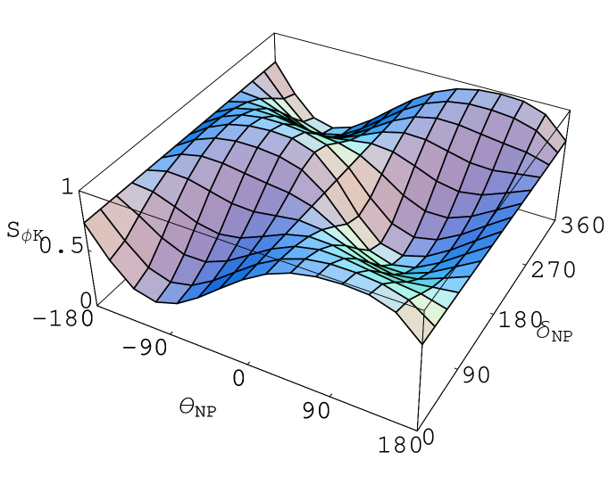
Now taking $r_{NP}=0.28$ and varying the weak phase $\theta_{NP}=\{-\pi,\pi\}$ and strong phase $\delta_{NP}=\{0,2\pi\}$ according to Eq. (16), we find that the value of $S_{\phi K}$ can not be negative as shown in Fig-1. Thus the observed value of $S_{\phi K}$ can not be accommodated in the THDM.

Figure 1: 3DPlot of $S_{\phi K}$ versus the weak phase $\theta_{NP}$ and strong phase $\delta_{NP}$ (in degrees) for $r_{NP}=0.28$

3.3 Contributions from Model with extra vector like down quark

Now we consider the model with an additional vector like down quark [34]. It is a simple model beyond the SM with an enlarged matter sector with an additional vector-like down quark $D_{4}$. The most interesting effects in this model concern CP asymmetries in neutral B decays into final CP eigenstates. At a more phenomenological level, models with isosinglet quarks provide the simplest self consistent framework to study deviations of $3\times 3$ unitarity of the CKM matrix as well as, allow flavor changing neutral currents at the tree level. The presence of an additional down quark implies a $4\times 4$ matrix $V_{i\alpha}$ $(i=u,c,t,4,~{}\alpha=d,s,b,b^{\prime})$, diagonalizing the down quark mass matrix. For our purpose, the relevant information for the low energy physics is encoded in the extended mixing matrix. The charged currents are unchanged except the $V_{CKM}$ is now the $3\times 4$ upper submatix of $V$. However, the distinctive feature of this model is that FCNC enters neutral current Lagrangian of the left handed downquarks :

$${\cal L}_{Z}=\frac{g}{2\cos\theta_{W}}\left[\bar{u}_{Li}\gamma^{\mu}u_{Li}-\bar{d}_{L\alpha}U_{\alpha\beta}\gamma^{\mu}d_{L\beta}-2\sin^{2}\theta_{W}J_{em}^{\mu}\right]Z_{\mu}$$ (30)

with

$$U_{\alpha\beta}=\sum_{i=u,c,t}V_{\alpha i}^{\dagger}V_{i\beta}=\delta_{\alpha\beta}-V_{4\alpha}^{*}V_{4\beta}$$ (31)

where $U$ is the neutral current mixing matrix for the down sector which is given above. As $V$ is not unitary, $U\neq{\bf{1}}$. In particular its non-diagonal elements do not vanish :

$$U_{\alpha\beta}=-V_{4\alpha}^{*}V_{4\beta}\neq 0~{}~{}~{}{\rm for}~{}\alpha\neq\beta$$ (32)

Since the various $U_{\alpha\beta}$ are nonvanishing they would signal new physics and the presence of FCNC at tree level, this can substantially modify the predictions for CP asymmetries. The new element $U_{sb}$ which is relevant to our study is given as

$$U_{sb}=V_{us}^{*}V_{ub}+V_{cs}^{*}V_{cb}+V_{ts}^{*}V_{tb}$$ (33)

The decay mode $B^{0}\to\phi K_{S}$ receives the new contributions both from color allowed and color suppressed $Z$-mediated FCNC transitions. The new additional operators are given as

$$O_{1}^{Z-FCNC}=[\bar{s}_{\alpha}\gamma^{\mu}(1-\gamma_{5})b_{\alpha}][\bar{s}_{\beta}\gamma_{\mu}(C_{V}^{s}-C_{A}^{s}\gamma_{5})s_{\beta}]$$

$$O_{2}^{Z-FCNC}=[\bar{s}_{\beta}\gamma^{\mu}(1-\gamma_{5})b_{\alpha}][\bar{s}_{\alpha}\gamma_{\mu}(C_{V}^{s}-C_{A}^{s}\gamma_{5})s_{\beta}]$$ (34)

where $C_{V}^{s}$ and $C_{A}^{s}$ are the vector and axial vector $Zs\bar{s}$ couplings. Using Fierz transformation and the identity $(C_{V}^{s}-C_{A}^{s}\gamma_{5})=[(C_{V}^{s}+C_{A}^{s})(1-\gamma_{5})+(C_{V}^{s}-C_{A}^{s})(1+\gamma_{5})]/2$, the matrix elements of the operators are given as

$$\langle\phi\bar{K}^{0}|O_{1}^{Z-FCNC}|\bar{B}^{0}\rangle = \left[\frac{4}{3}\frac{(C_{V}^{s}+C_{A}^{s})}{2}+\frac{(C_{V}^{s}-C_{A}^{s})}{2}\right]X$$

$$\langle\phi\bar{K}^{0}|O_{2}^{Z-FCNC}|\bar{B}^{0}\rangle = \left[\frac{4}{3}\frac{(C_{V}^{s}+C_{A}^{s})}{2}+\frac{1}{3}\frac{(C_{V}^{s}-C_{A}^{s})}{2}\right]X$$ (35)

The values for $C_{V}^{s}$ and $C_{A}^{s}$ are taken as

$$C_{V}^{s}=-\frac{1}{2}+\frac{2}{3}\sin^{2}\theta_{W}\;,~{}~{}~{}~{}~{}~{}~{}~{}~{}C_{A}^{s}=-\frac{1}{2}\;.$$ (36)

Thus the amplitude for $B\to\phi K$ arising from the $Z$ mediated FCNC tree diagram is given as

$$A^{VLDQ}(\bar{B}^{0}\to\phi\bar{K}_{0})=\frac{G_{F}}{\sqrt{2}}~{}\frac{4}{3}\left(-1+\sin^{2}\theta_{W}\right)U_{sb}X\;.$$ (37)

Using the experimental upper limit $Br(B\to X_{s}l^{+}l^{-})<4.2\times 10^{-5}$ [36], in Ref. [35] the bound on $|U_{bs}|$ is found to be $|U_{bs}|\leq 2\times 10^{-3}$. Recently Belle Collaboration [37] has measured the branching ratio for the process $B\to X_{s}l^{+}l^{-}$ as

$$Br(B\to X_{s}l^{+}l^{-})=(6.1\pm 1.4^{+1.4}_{-1.1})\times 10^{-6}$$ (38)

Using the above result one can obtain the value [35, 38]

$$|Y_{0}(x_{t})~{}\lambda_{t}^{bs}+C_{U2Z}~{}U_{bs}|=0.06\pm 0.03\;,$$ (39)

where all the parameters in (39) are given in [35]. Thus one obtains the value of $U_{bs}$ as

$$|U_{bs}|\simeq 1\times 10^{-3}$$ (40)

Now using $\sin^{2}\theta_{W}$=0.23, we find

$$r_{NP}\simeq 0.58$$ (41)

Figure 2: 3DPlot of $S_{\phi K}$ versus the weak phase $\theta_{NP}$ and strong phase $\delta_{NP}$ (in degrees) for $r_{NP}=0.58$

Figure 3: Branching ratio of $B\to\phi K^{0}$ process (in units of $10^{-5}$) versus the phase $\phi_{NP}$ (in degree). The horizontal solid line is the central experimental value whereas the dashed horizontal lines denote the error limits.

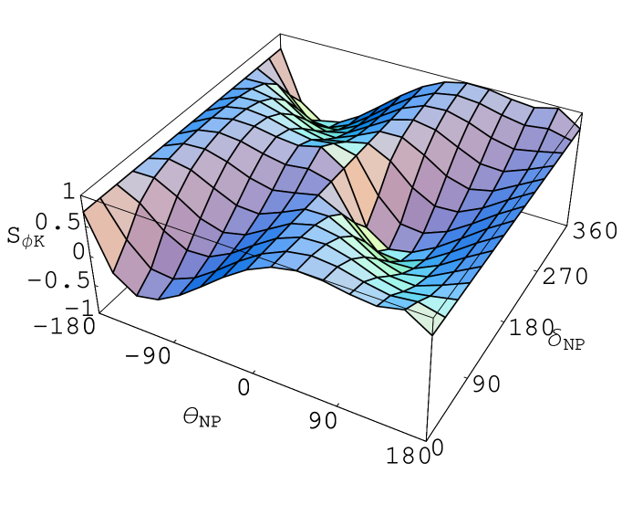
The variation of $S_{\phi K}$ with respect to strong phase $\delta_{NP}$ and weak phase $\theta_{NP}$ according to Eq. (16) in VLDQ model is shown in Figure-2 and the variation of branching ratio (15) is shown in Fig-3. It can be seen from the figures that the observed asymmetry $S_{\phi K}$ and the branching ratio can be easily accommodated in this model.

4 CP Violation in $B\to\eta^{\prime}K_{S}$ process

At this stage we are in a position to test, as mentioned earlier, whether the above two models (Model-III of THDM and VLDQ) can accommodate the result for another similar mode, which seems to be in agreement with the SM. In doing so, now we consider the $B^{0}\to\eta^{\prime}K^{0}$ process.

4.1 Contributions from SM and THDM

In the SM, in addition to $b\to s\bar{q}q$ ( $q=(u,d,s)$) penguins, the $B^{0}\to\eta^{\prime}K_{S}$ process also receives a small contribution from color suppressed $b\to u\bar{u}s$ tree diagram. We first find out the standard model contribution. The matrix element in the SM is given as

$$A(\bar{B}^{0}\to\eta^{\prime}\bar{K}^{0}) = \frac{G_{F}}{\sqrt{2}}\biggr{[}V_{ub}V_{us}^{*}\sum_{i=1}^{2}C_{i}^{eff}\langle\eta^{\prime}\bar{K}^{0}|O_{i}|\bar{B}^{0}\rangle$$ (42)

$$- V_{tb}V_{ts}^{*}\sum_{i=3}^{10}C_{i}^{eff}\langle\eta^{\prime}\bar{K}^{0}|O_{i}|\bar{B}^{0}\rangle\biggr{]}\;,$$

where $O_{1,2}$ are the tree and $O_{3-6(7-10)}$ are the QCD (electroweak) penguin operators. The matrix elements of these operators are given in the factorization approximation as [14]

$$\langle\eta^{\prime}\bar{K}^{0}|O_{1}|\bar{B}^{0}\rangle=\frac{1}{3}X_{2}~{}~{}~{}~{}~{}~{}\langle\eta^{\prime}\bar{K}^{0}|O_{2}|\bar{B}^{0}\rangle=X_{2}$$

$$\langle\eta^{\prime}\bar{K}^{0}|O_{3}|\bar{B}^{0}\rangle=\frac{1}{3}X_{1}+2X_{2}+\frac{4}{3}X_{3}$$

$$\langle\eta^{\prime}\bar{K}^{0}|O_{4}|\bar{B}^{0}\rangle=X_{1}+\frac{2}{3}X_{2}+\frac{4}{3}X_{3}$$

$$\langle\eta^{\prime}\bar{K}^{0}|O_{5}|\bar{B}^{0}\rangle=\frac{R_{1}}{3}X_{1}-2X_{2}-\left(1-\frac{R_{2}}{3}\right)X_{3}$$

$$\langle\eta^{\prime}\bar{K}^{0}|O_{6}|\bar{B}^{0}\rangle=R_{1}X_{1}-\frac{2}{3}X_{2}-\left(\frac{1}{3}-R_{2}\right)X_{3}$$

$$\langle\eta^{\prime}\bar{K}^{0}|O_{7}|\bar{B}^{0}\rangle=\frac{1}{2}\biggr{[}-\frac{R_{1}X_{1}}{3}-X_{2}+\left(1-\frac{R_{2}}{3}\right)X_{3}\biggr{]}$$

$$\langle\eta^{\prime}\bar{K}^{0}|O_{8}|\bar{B}^{0}\rangle=\frac{1}{2}\biggr{[}-R_{1}X_{1}-\frac{X_{2}}{3}+\left(\frac{1}{3}-R_{2}\right)X_{3}\biggr{]}$$

$$\langle\eta^{\prime}\bar{K}^{0}|O_{9}|\bar{B}^{0}\rangle=\frac{1}{2}\biggr{[}-\frac{X_{1}}{3}+X_{2}-\frac{4}{3}X_{3}\biggr{]}$$

$$\langle\eta^{\prime}\bar{K}^{0}|O_{10}|\bar{B}^{0}\rangle=\frac{1}{2}\biggr{[}-X_{1}+\frac{X_{2}}{3}-\frac{4}{3}X_{3}\biggr{]}$$ (43)

where

$$X_{1} = i(m_{B}^{2}-m_{\eta^{\prime}}^{2})F_{0}^{B\to\pi}(m_{K^{0}}^{2})\frac{X_{\eta^{\prime}}}{\sqrt{2}}f_{K}$$

$$X_{2} = i(m_{B}^{2}-m_{K^{0}}^{2})F_{0}^{B\to K}(m_{\eta^{\prime}}^{2})\frac{X_{\eta^{\prime}}}{\sqrt{2}}f_{\pi}$$

$$X_{3} = i(m_{B}^{2}-m_{K^{0}}^{2})F_{0}^{B\to K}(m_{\eta^{\prime}}^{2})Y_{\eta^{\prime}}\sqrt{2f_{K}^{2}-f_{\pi}^{2}}$$

$$R_{1} = \frac{2m_{K^{0}}^{2}}{(m_{b}-m_{d})(m_{s}+m_{d})}\;,~{}~{}~{}~{}~{}~{}R_{2}=\frac{2(2m_{K^{0}}^{2}-m_{\pi}^{2}}{(m_{b}-m_{s})(m_{s}+m_{s})}\;.$$ (44)

$X_{\eta^{\prime}}=0.57$ and $Y_{\eta^{\prime}}=0.82$ are the mixing parameters of the $u\bar{u}+d\bar{d}$ and $s\bar{s}$ components in the $\eta^{\prime}$ meson [39], which correspond to $\theta_{P}=-20^{\circ}$. Thus the amplitude is given as

$$A(B^{0}\to\eta^{\prime}K^{0}) = i\frac{G_{F}}{2}\biggr{[}V_{ub}V_{us}^{*}a_{2}X_{2}-V_{tb}V_{ts}^{*}\biggr{\{}\left(a_{4}-\frac{a_{10}}{2}+\left(a_{6}-\frac{a_{8}}{2}\right)R_{1}\right)X_{1}$$ (45)

$$+ \left(2(a_{3}-a_{5})-\frac{1}{2}(a_{7}-a_{9})\right)X_{2}$$

$$+ \left(a_{3}+a_{4}-a_{5}+\frac{1}{2}(a_{7}-a_{9}-a_{10})+\left(a_{6}-\frac{a_{8}}{2}\right)R_{2}\right)X_{3}\biggr{\}}\biggr{]}$$

The decay width can be given by

$$\Gamma(B^{0}\to\eta^{\prime}K^{0})=\frac{|\vec{p}|}{8\pi m_{B}^{2}}|A(B^{0}\to\eta^{\prime}K^{0})|^{2}$$ (46)

Using $F_{0}^{(B\to\pi)}(m_{K^{0}}^{2})=0.335$, $f_{K(\pi)}=0.16(0.13)$ GeV, the quark masses as $(m_{d},~{}m_{s},~{}m_{b})=(0.0076,~{}0.122,~{}4.88)$ GeV and the values of the coefficients $a_{i}$’s for $N_{C}=3$ from Ref. [27] we obtain the branching ratio in the standard model as

$$BR(B^{0}\to\eta^{\prime}K^{0})|_{SM}=3.24\times 10^{-5}\;.$$ (47)

which is slightly less than the current experimental data [28]

$$BR(B^{0}\to\eta^{\prime}K^{0})=(5.8_{-1.3}^{+1.4})\times 10^{-5}\;.$$ (48)

Now we consider the contributions arising from THDM. As discussed earlier in this case due to the presence of new charged Higgs penguin diagrams, the values of the effective Wilson coefficients $a_{i}$’s get modified. Again substituting their values from [27] in Eq. (45), we obtain the transition amplitude as

$$A^{THDM}(B^{0}\to\eta^{\prime}K^{0})=A^{SM}(1+0.27~{}e^{i(\theta_{NP}+\delta_{NP})})\;.$$ (49)

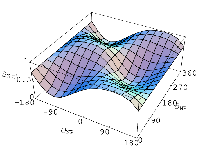
Now taking $r_{NP}=0.27$ and varying the weak phase $\theta_{NP}=\{-\pi,\pi\}$ and strong phase $\delta_{NP}=\{0,2\pi\}$ we can see from Figure-4, that the observed value of $S_{\eta^{\prime}K}$ can be accommodated in the THDM. Furthermore, the observed branching ratio can also be explained in this model as seen from from Figure-5. If we take a crude assumption that the THDM and SM amplitudes interfere constructively, the maximum value of branching ratio is found to be

$$BR^{THDM}(B^{0}\to\eta^{\prime}K^{0})=5.22\times 10^{-5}\;,$$ (50)

which lies within the present experimental limits [28].

Figure 4: 3DPlot of $S_{\eta^{\prime}K}$ versus the weak phase $\theta_{NP}$ and strong phase $\delta_{NP}$ (in degrees) for $r_{NP}=0.27$

Figure 5: Branching ratio of $B^{0}\to\eta^{\prime}K^{0}$ (in units of $10^{-5}$) process in THDM versus the phase $\phi_{NP}$ (in degree). The horizontal solid line is the central experimental value whereas the dashed horizontal lines denote the error limits.

4.2 Contributions from VLDQ Model

Now we consider the contributions arising from extra vector like down quark model. In this case the $B^{0}\to\eta^{\prime}K^{0}$ process proceeds through both color allowed and color suppressed tree level $Z$-mediated FCNC diagrams. The corresponding operators are given as

$$O_{1}^{Z-FCNC}=[\bar{s}_{\alpha}\gamma^{\mu}(1-\gamma_{5})b_{\alpha}][\bar{q}_{\beta}\gamma_{\mu}(C_{V}^{q}-C_{A}^{q}\gamma_{5})q_{\beta}]$$

$$~{}~{}~{}~{}~{}~{}~{}~{}~{}\equiv[\bar{s}_{\alpha}\gamma^{\mu}(1-\gamma_{5})b_{\alpha}]\left[\bar{q}_{\beta}\gamma_{\mu}\left\{\frac{(C_{V}^{q}+C_{A}^{q})}{2}(1-\gamma_{5})+\frac{(C_{V}^{q}-C_{A}^{q})}{2}(1+\gamma_{5})\right\}q_{\beta}\right]$$

$$O_{2}^{Z-FCNC}=[\bar{s}_{\beta}\gamma^{\mu}(1-\gamma_{5})b_{\alpha}][\bar{q}_{\alpha}\gamma_{\mu}(C_{V}^{q}-C_{A}^{q}\gamma_{5})q_{\beta}]$$

$$~{}~{}~{}~{}~{}~{}~{}~{}\equiv[\bar{s}_{\beta}\gamma^{\mu}(1-\gamma_{5})b_{\alpha}][\bar{q}_{\alpha}\gamma_{\mu}\left\{\frac{(C_{V}^{q}+C_{A}^{q})}{2}(1-\gamma_{5})+\frac{(C_{V}^{q}-C_{A}^{q})}{2}(1+\gamma_{5})\right\}q_{\beta}]$$ (51)

Using Fierz transformation and equation of motion the matrix elements of these operators are given as

$$\langle\eta^{\prime}\bar{K}^{0}|O_{1}^{Z-FCNC}|\bar{B}^{0}\rangle = (C_{A}^{u}+C_{A}^{d})X_{2}+C_{A}^{s}X_{3}$$ (52)

$$+ \frac{1}{6}\biggr{[}\left(C_{V}^{d}(1+R_{1})+C_{A}^{d}(1-R_{1})\right)X_{1}$$

$$+ \biggr{(}C_{V}^{s}(1+R_{2})+C_{A}^{s}(1-R_{2})\biggr{)}X_{3}\biggr{]}$$

$$\langle\eta^{\prime}\bar{K}^{0}|O_{2}^{Z-FCNC}|\bar{B}^{0}\rangle = \frac{1}{3}(C_{A}^{u}+C_{A}^{d})X_{2}+\frac{1}{3}C_{A}^{s}X_{3}$$ (53)

$$+ \frac{1}{2}\biggr{[}\left(C_{V}^{d}(1+R_{1})+C_{A}^{d}(1-R_{1})\right)X_{1}$$

$$+ \biggr{(}C_{V}^{s}(1+R_{2})+C_{A}^{s}(1-R_{2})\biggr{)}X_{3}\biggr{]}$$

So the amplitude for $B^{0}\to\eta^{\prime}K^{0}$ in VLDQ model is given as

$$A^{VLDQ}(\bar{B}^{0}\to\eta^{\prime}\bar{K}^{0}) = \frac{G_{F}}{\sqrt{2}}U_{sb}\biggr{[}\frac{4}{3}\left\{(C_{A}^{u}+C_{A}^{d})X_{2}+C_{A}^{s}X_{3}\right\}$$ (54)

$$+ \frac{2}{3}\biggr{\{}\left(C_{V}^{d}(1+R_{1})+C_{A}^{d}(1-R_{1})\right)X_{1}$$

$$+ \biggr{(}C_{V}^{s}(1+R_{2})+C_{A}^{s}(1-R_{2})\biggr{)}X_{3}\biggr{\}}\biggr{]}$$

Substituting the values of $C_{V(A)}^{q}$ as

$$C_{V}^{u}=\frac{1}{2}-\frac{4}{3}\sin^{2}\theta_{W}\;,~{}~{}~{}~{}~{}~{}~{}~{}~{}C_{A}^{u}=\frac{1}{2}\;,$$

$$C_{V}^{(s,d)}=-\frac{1}{2}+\frac{2}{3}\sin^{2}\theta_{W}\;,~{}~{}~{}~{}~{}C_{A}^{(s,d)}=-\frac{1}{2}\;.$$ (55)

we find

$$r_{NP}\simeq 0.72$$ (56)

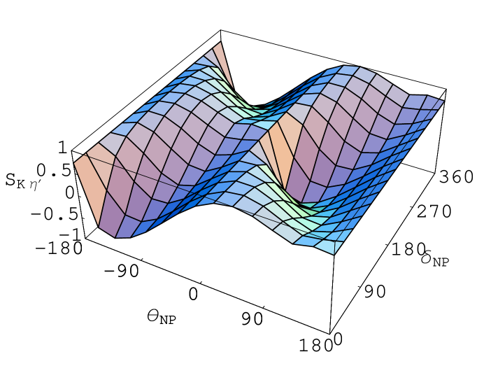
The variation of $S_{\eta^{\prime}K^{0}}$ and the branching ratio according to Eqs. (16) and (15)in the vector like down quark model are shown in Fig-6 and Fig-7. It can be seen that the observed asymmetry and branching ratio for $B^{0}\to\eta^{\prime}K^{0}$ mode can be easily accommodated in this model.

Figure 6: 3DPlot of $S_{\eta^{\prime}K^{0}}$ versus the weak phase $\theta_{NP}$ and strong phase $\delta_{NP}$ (in degrees) for $r_{NP}=0.72$

Figure 7: Branching ratio of $B^{0}\to\eta^{\prime}K^{0}$ process (in units of $10^{-5}$) in VLDQ model versus the phase $\phi_{NP}$ (in degree). The horizontal solid line is the central experimental value whereas the dashed horizontal lines denote the error limits.

5 Conclusions

To summarize, the time dependent CP asymmetry measurements in $B\to\phi K_{s}$ gives $\sin 2\beta$, which is 2.7$\sigma$ deviation from the corresponding value in $B\to\psi K_{S}$. According to the SM expectation they should measure the same. Unlike the $B\to\psi K_{S}$, which is a tree level process, $B\to\phi K_{S}$ occurs at one loop level, which allows room for new physics to play an important role. In this paper, we have explored two simple beyond SM scenarios, the two Higgs doublet model (model III) and model with extra vector like down quark. We found that model III of THDM is unable to explain, whereas vector like down quark model can easily explain the result.

It is important to note here that any new physics scenario that explains the $\phi K_{s}$ discrepancy must also explain another similar two-body decay $B\to\eta^{\prime}K_{s}$, which is also expected to give the same value as of $\psi K_{s}$ or $\phi K_{s}$, i.e., sin 2$\beta$. In doing so it will be easy to rule out or narrow down the various NP scenarios. We found that both the models (THDM-model-III and VLDQ) can explain the $\eta^{\prime}K_{s}$ result. This in turn gives us the clue that the VLDQ model may possibly be a strong contender for the NP effects responsible in $B\to\phi K_{s}$. It is worthwhile to emphasize that various supersymmetric models (as can be found in the literature) can explain the $\phi K_{s}$ discrepancy. But apart from [13, 14] none of the scenarios so far explained the simultaneous explanation of $\phi K_{s}$ and $\eta^{\prime}K_{s}$. On the other hand, our findings indicate that the simple non-supersymmetric extension of the SM in terms of the matter content should not be ignored for possible NP candidature. Regardless of the sources of NP, if in future the $\phi K_{s}$ result continues to be different from the SM expectation, then it will certainly establish the presence of NP.

6 Acknowledgements

We thank Yuval Grossman for fruitful discussions. The work of RM was supported in part by Department of Science and Technology, Government of India through Grant No. SR/FTP/PS-50/2001.

References

- [1] B. Aubert et al. [BABAR Collaboration], Phys. Rev. Lett. 89, 201802 (2002) [arXiv:hep-ex/0207042].
- [2] K. Abe et al. [Belle Collaboration], [arXiv:hep-ex/0207098].
- [3] Y. Nir, in Proceedings at the ICHEP 2002, Amsterdam, 2002 [arXiv:hep-ph/0208080].
- [4] N. Cabibbo, Phys. Rev. Lett. 10, 531 (1963); M. Kobayashi and T. Maskawa, Prog. Theor. Phys. 49, 652 (1973).
- [5] Y. Grossman and M. P. Worah, Phys. Lett. B 395, 241 (1997) [arXiv:hep-ph/9612269].
- [6] G. Hiller, Phys. Rev. D 66, 071502 (2002).
- [7] G. Barenboim, J. Bernabeu and M. Raidal, Phys. Rev. Lett. 80, 4625 (1998); M. Raidal, Phys. Rev. Lett. 89, 231803 (2002).
- [8] M. Ciuchini and L. Silverstini, Phys. Rev. Lett. 89, 231802 (2002); C.-W. Chiang and J. L. Rosner, [arXiv:hep-ph/0302094].
- [9] E. Lunghi and D. Wyler, Phys. Lett. B 521, 320 (2001); S. Khalil and E. Kou, Phys. Rev. D 67, 055009 (2003) [arXiv:hep-ph/0212023]; G. L. Kane, P. Ko, H. Yang, C. Kolda, J.-H. Park and L. T. Yang, Phys. Rev. Lett. 90, 141803 (2003); K Agashe and C. D Carone, [arXiv:hep-ph/0304229].
- [10] A. Datta, Phys. Rev. D 66, 071702(R) (2002).
- [11] S. Baek, [arXiv:hep-ph/0301269]
- [12] Y. Grossman, G. Isidori and M. Worah, Phys. Rev. D 58, 057504 (1997).
- [13] B. Dutta, C. S. Kim and S. Oh, Phys. Rev. Lett. 90, 011801 (2003); A Kundu, T. Mitra, [arXiv:hep-ph/0302123].
- [14] S. Khalil and E. Kou, [arXiv:hep-ph/0303214].
- [15] B. Aubert et al. [BABAR Collaboration], [arXiv:hep-ex/0207070].
- [16] R. A. Briere et al. [CLEO Collaboration], Phys. Rev. Lett. 86, 3718, (2001) [arXiv:hep-ex/0101032]; C. P. Jessop et al. [CLEO Collaboration], Phys. Rev. Lett. 85, 2881, (2001) [arXiv:hep-ex/0006008].
- [17] D. London and A. Soni, Phys. Lett. B 407, 61 (1997).
- [18] K. Abe et al. [Belle Collaborations], Phys. Rev. D 67, 031102 (2003) [arXiv:hep-ex/0212062].
- [19] B. Aubert et al. [BABAR Collaboration], [arXiv:hep-ex/0303046].
- [20] I. I. Bigi and A I. Sanda, CP Violation, Cambridge Monographs on Particle Physics, Nuclear Physics and Cosmology, (Cambridge University Press, Cambridge, England 2000); G. C. Branco, L. Lavoura and J. P. Silva, CP Violation, International Series of Monographs on Physics, Number 103, (Oxford University Press, New York 1999).
- [21] Y. Grossman, Z. Ligeti, Y. Nir and H. Quinn, [arXiv:hep-ph/0303171].
- [22] A. J. Buras and R. Fleischer, in Heavy Flavours II, eds. A. J. Buras and M. Lindner, World Scientific Singapore, page- 65.
- [23] G. Buchalla, A. J. Buras and M. E. Lautenbacher, Rev. Mod. Phys. 68, 1125 (1996).
- [24] A. Ali and C. Greub, Phys. Rev. D 57, 2996 (1998); A. Ali, G. Kramer and C. D. Lü, Phys. Rev. D 58, 094009 (1998).
- [25] G. Barenboim, J. Bernabeu, J. Matias and M. Raidal, Phys. Rev. D 60, 016003 (1999).
- [26] N.G. Deshpande and J. Trampetic, Phys. Rev. D 41, 2926 (1990); H. Simma and D. Wyler, Phys. Lett. B 272, 395 (1991); J.-M. Gerard and W.-S. Hou, Phys. Rev. D 43, 2909 (1991); Phys. Lett. B 253, 478 (1991).
- [27] Z. Xiao, C. S. Li and K.-T. Chao, Phys. Rev. D 63, 074005 (2001); ibid 65, 114021 (2002); [arXiv:hep-ph/0012269].
- [28] K Hagiwara et al, Particle Data Group, Phys. Rev. D 66, 010001 (2002).
- [29] J. F. Gunion, H. E. Haber, G. Kane and S. Dawson, The Higgs Hunter’s Guide, Addison-Wesley Publishing Company, (1990).
- [30] D. Atwood, L. Reina and A. Soni, Phys. Rev. D 55, 3156 (1997).
- [31] T. P. Cheng and M. Sher, Phys. Rev. D 35, 3484 (1987); M. Sher and Y. Yuan, Phys. Rev. D 44, 1461 (1991); W. S. Hou, Phys. Lett. B 296, 179 (1992); D. Chang, W. S. Hou and W. Y. Keung, Phys. Rev. D 48, 217 (1993); Y. L. Wu and L. Wolfenstein, Phys. Rev. Lett. 73, 1762 (1994); D. Atwood, L. Reina and A. Soni, Phys. Rev. Lett. 75, 3800 (1995).
- [32] D. B.-Chao, K. Cheung and W.-Y. Keung, Phys. Rev. D 59, 115006 (1999).
- [33] T. Inami and C. S. Lim, Prog. Theor. Phys. 65, 297 (1981); ibid 65, 1772E (1981).
- [34] Y. Grossman, Y. Nir and R. Rattazzi, in Heavy Flavours II, eds. A. J. Buras and M. Lindner, World Scietific Sigapore, page-755 [arXiv:hep-ph/9701231].
- [35] G. Barenboim, F. J. Bottella and O. Vives, Phys. Rev. D 64, 015007 (2001).
- [36] S Glenn et al. [CLEO Collaboration], Phys. Rev. Lett. 80, 2289 (1998).
- [37] J. Kaneko et al. [Belle Collaboration], Phys. Rev. Lett. 90, 021801 (2003).
- [38] G. Buchalla, G. Hiller and G. Isidori, Phys. Rev. D 63, 014015 (2001).
- [39] J. L. Rosner, Phys. Rev. D 27, 1101 (1983); E. Kou, Phys. Rev. D 63, 054027 (2001).