Light Scalar Mesons

in the Improved Ladder Approximation

of QCD

with Strong $U_{A}(1)$ Breaking

Toru Umekawa

Thesis submitted for the Degree

of Doctor of Science

Department of Physics, Tokyo Institute of Technology,

Meguro, Tokyo, 152-8551 Japan

January, 2003

Abstract

The spectrum and the mixing angle of the light scalar nonet mesons are studied using the extended Nambu-Jona-Lasinio (NJL) model as well as the improved ladder approximation (ILA) of QCD with $U_{A}(1)$  symmetry breaking interaction. The ILA is an approximation that is consistent with chiral symmetry and consists of the rainbow approximation of the Schwinger-Dyson equation and the ladder approximation of the Bethe-Salpeter equation. Improvement is made by the use of the running coupling constant according to the Higashijima-Miransky method. The $U_{A}(1)$  breaking is supposed to come from the coupling of light quarks to instanton, and is represented by a contact six-quark vertex, called the Kobayashi-Maskawa-’t Hooft (KMT) interaction. The strength of the KMT interaction in the NJL model is determined so as to reproduce the electromagnetic decays of the $\eta$ meson. That in the ILA approach is determined so as to reproduce the pseudoscalar meson spectrum. This interaction is so strong that it causes large mixing of $(u\bar{u}+d\bar{d})$ and $s\bar{s}$, in the $\eta$ meson.

In the extended NJL model, we study the qualitative features of the scalar meson spectrum. In the scalar nonet spectrum, the KMT interaction is found to give the right ordering of $\sigma-a_{0}$ masses and a few hundred MeV mass difference between the $\sigma$ and $a_{0}$ mesons. We also find that the strangeness content in the $\sigma$ meson is about $15\%$.

In the ILA approach, we confirm the qualitative features of the results from the extended NJL. We obtain the mass spectra of the light pseudoscalar nonet mesons and the $\sigma,a_{0}$ mesons which are consistent with current experimental data. They are both reproduced with the same parameter choice. On the other hand, we show that the obtained $f_{0}$ and $K_{0}^{*}$ state can not be identified directly with the experimental data. It may suggest that the $f_{0}(980)$ and $\kappa(700-900)$ states may not be explained only by the quark-anti quark state.

We also find that the strangeness content in the $\sigma$ meson is about $5\%$. We obtain the result that the $U_{A}(1)$ breaking interaction reproducing the mass spectrum of the pseudoscalar meson gives large effects on the scalar meson mass spectrum.

Chapter 1 Introduction

Understanding low-lying hadron spectrum is one of the most challenging problems in the quantum chromodynamics (QCD). The spectrum is highly nontrivial due to the nonperturbative complexity, such as dynamical chiral symmetry breaking (D$\chi$SB), axial U(1) anomaly. For instance, the pseudoscalar mesons are off-scale light, if we suppose that they are bound states of a quark and an antiquark, while their spin-flip partners, i.e., vector mesons, are normal with masses about 2/3 of the baryon masses. This “anomaly” in the pseudoscalar mesons is attributed to their Nambu-Goldstone-boson nature associated with the D$\chi$SB. This is strongly in contrast with the heavy meson spectroscopy, such as heavy quarkonia and heavy flavor mesons. There the spectrum is more like the hydrogen atom with slightly stronger fine and hyperfine splittings.

It should be noticed that the low-lying hadrons are the key to explore the complicated QCD vacuum, as in QCD we are not able to “measure” the bulk properties of the ground state, which can be accessed directly in the case of condensed matter physics. Thus it is important to explore the properties of the low-lying hadrons from the viewpoints of QCD dynamics and symmetries.

Another nontrivial effect comes from $U_{A}(1)$ symmetry, which is expected to be broken by anomaly. Weinberg showed that the mass of $\eta^{\prime}$ should be less than $\sqrt{3}m_{\pi}$ if $U_{A}(1)$ symmetry were not explicitly broken.[1] Thus the $U_{A}(1)$ symmetry must be broken. Later, ’t Hooft pointed out the relation between $U_{A}(1)$ anomaly and topological gluon configurations of QCD and showed that the interaction of light quarks and instantons breaks the $U_{A}(1)$ symmetry.[2] He also showed that such interaction can be represented by a local $2N_{f}$ quark vertex, which is antisymmetric under flavor exchanges, in the dilute instanton gas approximation. The dynamics of instantons in the multi-instanton vacuum has been studied by many authors, either in the models or in the lattice QCD approach, and the widely accepted picture is that the QCD vacuum consists of small instantons of the size about 1/3 fm with the density of 1 instanton (or anti-instanton) per fm⁴.[3]

According to such instanton vacuum picture, the hadron spectrum shows its signature. The $\eta-\eta^{\prime}$ mass difference is the obvious one, which can be understood by flavor mixing in the $I=0$ ${1\over\sqrt{2}}\left(u\mbox{$\bar{u}$}+d\mbox{$\bar{d}$}\right)$ and $s\mbox{$\bar{s}$}$. Without the flavor mixing, ${1\over\sqrt{2}}\left(u\mbox{$\bar{u}$}+d\mbox{$\bar{d}$}\right)$ and $s\mbox{$\bar{s}$}$ would form mass eigenstates, and thus the ideal mixing is achieved. This is natural if the Okubo-Zweig-Iizuka (OZI) rule applies. However, the OZI rule is known to be significantly broken in the pseudoscalar mesons. For instance in the Nambu-Jona-Lasinio(NJL) model, the electromagnetic $\eta$ decay processes suggest that the mixing of ${1\over\sqrt{2}}\left(u\mbox{$\bar{u}$}+d\mbox{$\bar{d}$}\right)$ and $s\mbox{$\bar{s}$}$ is indeed strong so that the $\eta$ meson is close to the pure octet state.[4]

Recently, the scalar mesons, $J^{\pi}=0^{+}$, attracts a lot of attention by two reasons.[5] (1) Experimental evidence for $\sigma$ ($I=0$) scalar meson of mass around 500-800 MeV is overwhelming.[6, 7] Especially the decays of heavy mesons show clear peaks in the $\pi\pi$ invariant mass spectrum. (2) The roles of the scalar mesons in chiral symmetry have been stressed in the context of high temperature and/or density hadronic matter.[8] It is believed that chiral symmetry will be restored in the QCD ground state at high temperature (and/or baryon density). Above the critical temperature of order 150 MeV the world is nearly chiral symmetric and we expect that hadrons belong to an irreducible representation of chiral symmetry, if we neglect small mixing due to finite quark mass. The pion is not any more a Nambu-Goldstone(NG) boson, and has a finite mass and should be degenerate with a scalar meson, i.e., $\sigma$.

For $N_{f}=3$, we expect to have a $U(3)$ nonet of light scalar mesons, which are the chiral partners of the pseudoscalar nonet. We assume that $\sigma$ is the member of this nonet. The naive assignment of the flavor component of $\sigma(I=0)$ and $a_{0}(I=1)$ is $u\bar{u}+d\bar{d}$ and $u\bar{u}-d\bar{d}$, respectively. The masses of the $u\bar{u}+d\bar{d}$ and $u\bar{u}-d\bar{d}$ mesons must become degenerate, if the flavor mixing interaction is absent. However, the mass of $a_{0}(980)$, which is the lightest $a_{0}$ meson, is larger than that of $\sigma$ by about $400[\mbox{MeV}]$. We consider that this mass splitting is explained again by the $U_{A}(1)$ breaking interaction. As is in the case of the light pseudoscalar mesons, the $U_{A}(1)$ breaking interaction contributes significantly for the light scalar meson nonet and then $\sigma-a_{0}$ mass splitting is explained by the flavor mixing. The goal of this paper is to study the role of the $U_{A}(1)$  breaking interaction to the mass spectrum of the light nonet scalar meson. Here we study the lowest scalar meson states in the $I=0,\,1,\,1/2$ channels and the second lowest one in $I=0$ channel which we call $\sigma$, $a_{0}$, $K_{0}^{*}$ and $f_{0}$, respectively. The identification of these states with the experimentally observed states will be given later.

We first employ a simple model, the extended Nambu-Jona-Lasinio(NJL) model. It is the simplest possible quark model with the correct symmetry structure for the present purposes. [11] The chiral symmetry is broken both explicitly by the quark mass term and dynamically by quark loops, while the $U_{A}(1)$ symmetry is broken by the Kobayashi-Maskawa-’t Hooft (KMT) interaction. [2, 12] The KMT interaction is a contact six-quark interaction, which represents the $U_{A}(1)$  breaking effects induced by the instanton configuration of the gluon in the vacuum.

After understanding the qualitative features of the scalar meson spectrum in the extended NJL model, we proceed to the analysis using the improved ladder approximation (ILA) [14] of QCD with the KMT interaction. The ILA of QCD is the approximation in which the gluon is integrated out and is written only in terms of the quark degrees of freedom. The ILA is an approximation that is consistent with chiral symmetry. We employ the rainbow approximation of the Schwinger-Dyson (SD) equation for the quark propagator and the ladder approximation of the Bethe-Salpeter (BS) equation for the quark-anti quark bound state. It is important to note that these two approximated equations are consistent with the chiral symmetry. Improvement is made by the use of the running coupling constant according to the Higashijima-Miransky [13] method. The KMT interaction is introduced in the ILA as an explicit interaction kernel. Naito et al. [17, 18] showed explicitly that the chiral symmetry is indeed preserved in this formulation and properties of the pseudoscalar meson, such as the masses and decay constants, are consistent with those of the Nambu-Goldstone (NG) bosons of chiral symmetry breaking. They furthermore considered effects of the $U_{A}(1)$ breaking and explicit chiral symmetry breaking due to the finite quark masses. They successfully reproduced the realistic mass spectrum of the pseudoscalar mesons.

In this thesis, we consider the scalar mesons in the same formulation. The advantage of this approach is consistency with chiral symmetry. It is found that the properties of the light pseudoscalar mesons are reproduced according to the expectations from chiral symmetry. We then treat the scalar mesons and the pseudoscalar mesons as the chiral partners. In this study, at first we fix the parameters so that the mass spectrum and the decay constants of the pseudoscalar mesons are reproduced and then we apply those for the scalar mesons.

This subject has been studied in other approaches by many authors. The most direct approach might be the lattice QCD simulation. At present, however, it is difficult to compute the light singlet scalar meson. There have been studies by using the NJL model [19, 21] or the linear sigma model [22]. In those studies, the effects of the $U_{A}(1)$  breaking interaction are weak so that the flavor mixing in the $\sigma$ meson is negligible. However, recently Takizawa et al. [4] showed that the $U_{A}(1)$  breaking effects must be much stronger in order to explain the electromagnetic decays of the $\eta$ meson. The main aim of this study is to explain the anomalous ordering of scalar meson can be explained by the strong $U_{A}(1)$ breaking effects. Indeed we will show that the $\sigma-a_{0}$ splitting and significant flavor mixing is induced by the strong $U_{A}(1)$ breaking interaction. We will see a large mixing of $s\mbox{$\bar{s}$}$ component in the $\sigma$ meson in our approach.

Other pictures of the light scalar mesons proposed so far include the multi-quark state or the meson molecule state [9]. There may exist the mixing of quark-anti quark state with these state. However, it is difficult to believe that these multi-quark states are the main component of the light scalar mesons. We will show that the scalar meson nonet can be explained purely as the quark - anti quark state with the $U_{A}(1)$  breaking effects.

In chapter 2, we explain the theoretical background for this study. In chapter 3, we present the extended NJL model analysis. In chapter 4, we present the formulation of the ILA approach. In chapter 5, we show our results and give discussions on the mass spectrum as well as the mixings. In chapter 6, conclusions are given.

Chapter 2 Theoretical Background

2.1 Quantum Chromodynamics

Quantum Chromodynamics (QCD) is the $SU(3)$ nonabelian gauge field theory, which describes the strong interactions of colored quarks and gluons. A quark comes in 3 colors and gluons come in eight colors. Hadrons are color singlet combination of quarks, anti-quarks and gluons.

The Lagrangian of QCD with the gauge fixing terms is

$${\cal L}= \bar{\psi}({i}D\!\!\!\!/-m_{0})\psi-\frac{1}{4}F_{a}^{\mu\nu}F^{a}_{\mu\nu}-\frac{1}{2\xi_{0}}(\partial_{\mu}A^{\mu}_{a})^{2}$$ (2.1)

$$+\partial_{\mu}\bar{c}_{a}\partial^{\mu}c_{a}+g_{0}f_{abe}A_{a}^{\mu}(\partial_{\mu}\bar{c}_{b})c_{e}$$

$$F_{\mu\nu}^{a}=\partial_{\mu}A_{\nu}^{a}-\partial_{\nu}A_{\mu}^{a}-g_{0}f^{abc}A_{\mu}^{b}A_{\nu}^{c}$$ (2.2)

$$D_{\mu}=\partial_{\mu}+ig_{0}\frac{\lambda^{a}}{2}A_{\mu}^{a}$$ (2.3)

where $g_{0}$ is the QCD coupling constant, and the $f_{abc}$ is the structure constant of the $SU(3)$ algebra. The $\psi_{j}$ represent the quark fields in which the $j=1,2,3$ is the color label. The $A_{\mu}^{a}$ represent the gluon fields with $a=1,...,8$. The quantities $c_{a}$ are called ghost fields which are introduced by in gauge fixing procedure. The ghost occurs only in loops, and never appears as asymptotic state. The $\xi_{0}$ is the gauge fixing parameter. The limit $\xi_{0}\to\infty$ defines the Landau gauge and we use this gauge in the improved ladder approximation later.

The most characteristic property of QCD, which supports that the theory describing the dynamics of the hadron is QCD, is the asymptotic freedom. From the experiments of the deep inelastic scattering of the lepton from the hadron, it was found that the quarks are almost free in high momentum transfer region. This property is called asymptotic freedom and it was shown that only the nonabelian gauge field theory exhibits it. Then the extra symmetry of the nonabelian gauge field theory is identified with color symmetry which is suggested by the quark model. This completes QCD.

To see the asymptotic freedom nature of QCD we show the running coupling constant $\alpha_{s}(q^{2})\equiv g^{2}_{R}(q^{2})/4\pi$. It is obtained by the one-loop renormalization group calculation as

$$\alpha_{s}(q^{2})=\frac{12\pi}{(33-2N_{f})\ln(q^{2}/\Lambda^{2})}+\cdots$$ (2.4)

where $N_{f}$ is the number of quark flavors with mass less than $\sqrt{q^{2}}$. The $\alpha_{s}(q^{2})$ is small at large $q^{2}$. Consequently in the high energy region, the perturbative analysis of QCD makes sense and it is applied to the deep inelastic scattering, $e^{+}e^{-}$ annihilation process, decays of heavy quarkonia and so on.

In contrast, the $\alpha_{s}(q^{2})$ becomes large as $q^{2}$ decreases and then the perturbation approaches become poor approximations. In this region, the nonperturbative effects, especially the confinement and the dynamical chiral symmetry breaking, are important. The confinement means that only colorless states are physically realized and hence quarks cannot be observed in isolated state. The dynamical chiral symmetry breaking is explained in the next section. Because the complexity of low energy QCD, various approaches have been tried such as to solve QCD on the discretized space time numerically (lattice-gauge theory), construct effective theories and models (th potential quark model, the bag model, the Skyrme model, the NJL model), or to consider some limit as $N_{C}\to\infty$.

2.2 The Chiral Symmetry Breaking

If one supposes that all the masses of $N_{f}$ quarks are zero, the QCD Lagrangian satisfies ${U}_{fL}(N_{f})\times{U}_{fR}(N_{f})=U_{V}(1)\times U_{A}(1)\times{SU}_{fL}(N_{f})\times{SU}_{fR}(N_{f})$ symmetries, ie., the invariance under the transformations

$$\psi_{L}\equiv\frac{1}{2}(1-\gamma_{5})\psi \to \psi_{L}^{\prime}=\exp(i\theta_{L}^{a}\frac{\lambda^{a}_{f}}{2})\psi_{L}\qquad(a=0,...,N_{f}^{2}-1)$$ (2.5)

$$\psi_{R}\equiv\frac{1}{2}(1+\gamma_{5})\psi \to \psi_{R}^{\prime}=\exp(i\theta_{R}^{a}\frac{\lambda^{a}_{f}}{2})\psi_{R}\qquad(a=0,...,N_{f}^{2}-1).$$ (2.6)

Although the quark mass term breaks those symmetries explicitly, they remain approximate symmetries of QCD for light flavors i.e., $u,d$ and $s$.

Among these symmetries, some of them are broken in the vacuum state. The $U_{A}(1)$ symmetry is broken explicitly by the anomaly and we explain it in the next section.

We here concentrate on the ${SU}_{fL}(3)\times{SU}_{fR}(3)$ chiral symmetry, which is broken spontaneously in the vacuum. Then the symmetries of the QCD vacuum are $U_{V}(1)\times{SU}_{f}(3)$. In this section, we explain the chiral symmetry and its breaking in the case of $N_{f}=2$ for simplicity. At first, we show it using two simple models, the linear sigma model and the two-flavor Nambu-Jona-Lasinio (NJL) model, which have the $SU(2)_{L}\times SU(2)_{R}$ chiral symmetry. Then we explain the chiral symmetry of QCD.

The Lagrangian of the linear sigma model is

$${\cal L}= \bar{\psi}\i\partial\!\!\!/\psi+\frac{1}{2}\partial_{\mu}{\mbox{{\boldmath$\pi$}}}\partial^{\mu}{\mbox{{\boldmath$\pi$}}}+\frac{1}{2}\partial_{\mu}\sigma\partial^{\mu}\sigma-g\bar{\psi}(\sigma-i{\mbox{{\boldmath$\tau$}}\cdot\mbox{{\boldmath$\pi$}}}\gamma_{5})\psi$$ (2.7)

$$+\frac{\mu^{2}}{2}(\sigma^{2}+\mbox{{\boldmath$\pi$}}^{2})-\frac{\lambda}{4}(\sigma^{2}+\mbox{{\boldmath$\pi$}}^{2})^{2}$$

where $\psi$ is the doublet nucleon $\psi=\ ^{T}(p\ n)$ and $\pi$ is the triplet of the pion fields $\mbox{{\boldmath$\pi$}}=\ ^{T}(\pi^{1}\ \pi^{2}\ \pi^{3})$. This Lagrangian is invariant under the ${SU}_{fL}(2)\times{SU}_{fR}(2)$ chiral transeformation,

$$\psi_{L,R}\to{\psi^{\prime}}_{L,R}=U_{L,R}\psi_{L,R}\qquad\Sigma\equiv(\sigma+i\mbox{{\boldmath$\tau$}}\cdot\mbox{{\boldmath$\pi$}})\to\Sigma^{\prime}=U_{L}\Sigma U_{R}^{\dagger}$$ (2.8)

$$U_{L,R}=\exp(i\theta^{a}_{L,R}\frac{\tau^{a}}{2}).$$ (2.9)

It should be noted that this symmetry is isomorphic to $O(4)$ symmetry, which is represented by the 4-dimensional $(\sigma,\mbox{{\boldmath$\pi$}})$ space. When $\mu^{2}$ is positive. the potential energy

$$V(\sigma,\mbox{{\boldmath$\pi$}})=\frac{\mu^{2}}{2}(\sigma^{2}+\mbox{{\boldmath$\pi$}}^{2})-\frac{\lambda}{4}(\sigma^{2}+\mbox{{\boldmath$\pi$}}^{2})^{2}$$ (2.10)

forms a 4-dimensional wine bottle shape.

The classical minimum of $V(\sigma,\mbox{{\boldmath$\pi$}})$ gives the set of degenerate ground states satisfying

$$\sigma^{2}+\mbox{{\boldmath$\pi$}}^{2}=\frac{\mu^{2}}{\lambda}.$$ (2.11)

Let us choose a particular ground state,

$$\left\langle\sigma\right\rangle=\sqrt{\frac{\mu^{2}}{\lambda}}\equiv v,\quad\left\langle\mbox{{\boldmath$\pi$}}\right\rangle=0$$ (2.12)

Then one sees that the chiral $SU(2)_{fL}\times SU(2)_{fR}$ symmetry is broken spontaneously by the ground state $(\ref{Eq:sigmaGround})$. Defining $\tilde{\sigma}=\sigma-v$, we then rewrite the Lagrangian as

$${\cal L}= \psi(i\partial\!\!\!/-gv)\psi+\frac{1}{2}[\partial_{\mu}\tilde{\sigma}\partial^{\mu}\tilde{\sigma}-2\mu^{2}\tilde{\sigma}^{2}]+\frac{1}{2}\partial_{\mu}\mbox{{\boldmath$\pi$}}\cdot\partial^{\mu}\mbox{{\boldmath$\pi$}}$$ (2.13)

$$-g\bar{\psi}(\tilde{\sigma}-i{\mbox{{\boldmath$\tau$}}\cdot\mbox{{\boldmath$\pi$}}}\gamma_{5})\psi+\lambda v\tilde{\sigma}(\sigma^{2}+\mbox{{\boldmath$\pi$}}^{2})-\frac{\lambda}{4}[(\tilde{\sigma}^{2}+\mbox{{\boldmath$\pi$}}^{2})^{2}-v^{4}].$$

This Lagrangian is not any more symmetric under the rotation in the $(\tilde{\sigma},\mbox{{\boldmath$\pi$}})$ space. One sees that the pion becomes massless, while the scalar meson $\tilde{\sigma}$ acquires a mass $m_{\tilde{\sigma}}=\sqrt{2\mu^{2}}$, and also the fermion gets a mass $M=gv$.

The appearance of the massless pion is a concrete example of the Goldstone theorem: if a theory has a continuous symmetry of the Lagrangian is spontaneously broken, there must be a massless boson, which is called Nambu-Goldstone (NG) boson. In this case, the pion is the NG boson. The order parameter of the chiral symmetry breaking is $v=\left\langle\sigma\right\rangle$. In this model, the pion decay constant $f_{\pi}$ defined by

$$\left\langle 0|A_{\mu}^{i}|\pi^{j}(\mbox{{\boldmath$p$}})\right\rangle=if_{\pi}p_{\mu}\delta^{ij}$$ (2.14)

coincides with $v$ in the tree level.

Next we show the two flavor and $N_{C}$ color NJL model. This model is written in terms of quark degrees of freedom as

$${\cal L}=\psi(i\partial\!\!\!/)\psi+\frac{1}{2}g_{s}\sum_{i=0}^{3}\left[(\bar{\psi}\tau^{i}\psi)^{2}+(\bar{\psi}i\gamma_{5}\tau^{i}\psi)^{2}\right].$$ (2.15)

where $\psi=\ ^{T}(u\ d)$. This Lagrangian is invariant under the $U(2)_{fL}\times U(2)_{fR}$ chiral transformation

$$\psi_{L,R}\to{\psi^{\prime}}_{L,R}=\exp(i\theta_{L,R}^{i}\frac{\tau^{i}}{2})\psi_{L,R}\quad i=0,...,3.$$ (2.16)

In this case, the order parameter of the chiral symmetry breaking is the value of the composite operator $\left\langle\bar{\psi}\psi\right\rangle$ and then the symmetry is dynamically broken.

We analyze this model in the leading order of the $1/N_{C}$ expansion. Using the mean field approximation, the Lagrangian is rewritten as

$${\cal L}_{\rm MFA}=\bar{\psi}i\partial\!\!\!/q+M\bar{\psi}\psi$$ (2.18)

$$M\equiv-\frac{g_{s}}{N_{f}}\left\langle\bar{\psi}\psi\right\rangle=\frac{g_{s}}{N}\lim_{x\to 0}\mbox{tr}[S_{F}(x)]$$

. (2.19)

Eqs. $(\ref{Eq:NJL1})$ and $(\ref{Eq:NJL2})$ lead to the following equation for $M$:

$$M=4ig_{s}N_{C}\int\frac{d^{4}p}{(2\pi)^{4}}\frac{M}{p^{2}-M^{2}}$$ (2.20)

Rotating the integral into Euclidean space $(p^{0}\to ip_{4})$, we find the equation:

$$M=\frac{g_{s}N_{C}}{4\pi^{2}}\int_{0}^{\Lambda^{2}}dp^{2}\frac{p^{2}M}{p^{2}+M^{2}}$$ (2.21)

where $\Lambda$ is the ultraviolet cutoff. After the integral, we obtain

$$M(\kappa-1)=\kappa\frac{M^{3}}{\Lambda^{2}}\ln\frac{\Lambda^{2}+M^{2}}{M^{2}}$$ (2.22)

$$\kappa\equiv\frac{g_{s}N_{C}\Lambda^{2}}{4\pi^{2}}.$$ (2.23)

There is always the trivial solution, $M=0$, to this equation, and when $\kappa>1$, there is also a nontrivial one with $M\neq 0$. In the case of the $M\neq 0$, the value of $\left\langle\bar{\psi}\psi\right\rangle$ is not zero and it shows that the chiral $U_{fL}(2)\times U_{fR}(2)$ is dynamically broken to the $U_{fv}(2)$. The quarks acquire the dynamical mass $M$.

According to the dynamical symmetry breaking, there should be the four NG bosons. To confirm this, we consider the Bethe-Salpeter (BS) equations for the pseudoscalar mesons and the scalar mesons. The BS equation in the present model in Euclid space is written as

$${S_{F}}^{-1}_{n,n_{1}}(q+\frac{P}{2})\chi_{n_{1}m_{1}}(q,P){S_{F}}_{m_{1}m}^{-1}(q-\frac{P}{2})=\int\frac{d^{4}k}{(2\pi)^{4}}K_{mn,n_{2}m_{2}}(q,k;P)\chi_{n_{2},m_{2}}(q;P)$$

$$K_{mn,n_{2}m_{2}}=i\frac{g_{s}}{2}\left[(\tau^{j})_{nm}(\tau^{j})_{m_{2}n_{2}}+(i\gamma_{5}\tau^{j})_{nm}(i\gamma_{5}\tau^{j})_{m_{2}n_{2}}\right]$$ (2.24)

where $\chi$ is the BS amplitude defined as

$$\chi_{nm}(q;P)=e^{-iP\frac{x+y}{2}}\int d^{4}(x-y)\left\langle 0|T\bar{\psi}_{n}(x)\psi_{m}(y)|P\right\rangle e^{iq(x-y)}.$$ (2.25)

$|P\rangle$ is the bound state with momentum $P$. The BS amplitude for the pseudoscalar meson, ${\chi^{(P)}}_{i}$, and the BS amplitude for the scalar meson, ${\chi^{(S)}}_{i}$, can be written in terms of four scalar amplitudes as

$${\chi^{(P)}_{j}}_{nm}(q;P)=\mbox{{\boldmath$1$}}_{C}\frac{\tau_{j}}{2}\left[\phi^{(P)}_{S}(q;P)+\phi^{(P)}_{P}(q;P)q\!\!\!/+\phi^{(P)}_{Q}(q;P)P\!\!\!\!/+\phi^{(P)}_{T}(q;P)\frac{1}{2}(P\!\!\!\!/q\!\!\!/-q\!\!\!/P\!\!\!\!/)\right]\gamma_{5}$$

$${\chi_{j}^{(S)}}_{nm}(q;P)=\mbox{{\boldmath$1$}}_{C}\frac{\tau_{j}}{2}\left[\phi^{(S)}_{S}(q;P)+\phi^{(S)}_{P}(q;P)q\!\!\!/+\phi^{(S)}_{Q}(q;P)P\!\!\!\!/+\phi^{(S)}_{T}(q;P)\frac{1}{2}(P\!\!\!\!/q\!\!\!/-q\!\!\!/P\!\!\!\!/)\right]$$

where $\tau^{a}$ is the Pauli matrix which denotes the flavor structure of the meson state. In the chiral limit and in the leading order of the $1/N_{C}$ expansion, the BS equations becomes extremely simple. Furthermore we takes only the first order in $P^{2}/\Lambda^{2}$, then we obtain the following BS equation:

$$\left(q^{2}+\frac{P^{2}}{2}\right)\phi_{S}^{(P)}(q^{2},P^{2}) = \frac{\kappa}{\Lambda^{2}}\int^{\Lambda^{2}}dk^{2}k^{2}\phi_{S}^{(P)}(k^{2},P^{2})$$ (2.26)

$$\left(q^{2}+\frac{P^{2}}{2}+4M\right)\phi_{S}^{(S)}(q^{2},P^{2}) = \frac{\kappa}{\Lambda^{2}}\int^{\Lambda^{2}}dk^{2}k^{2}\phi_{S}^{(S)}(k^{2},P^{2}).$$ (2.27)

These equations are satisfied for each flavor $j$.

If one identifies the amputated function $\tilde{\chi}(q^{2})=(M^{2}-q^{2})\chi$ and substitute the $\frac{P^{2}}{2}\to M^{2}$, Eq. $(\ref{NJLBS_p})$ coincides with Eq. (2.20). Then we can easily solve it.

The spectrum of $M_{P}^{2}=-P^{2}$ of pseudoscalar bound states and the spectrum of $M_{S}^{2}=-P^{2}$ of scalar bound states are determined from the following equations

$$\kappa-1=\kappa\frac{M^{2}-\frac{M_{P}^{2}}{2}}{\Lambda^{2}}\ln\left(\frac{\Lambda^{2}+M^{2}-\frac{M_{P}^{2}}{2}}{M^{2}-\frac{M^{2}_{S}}{2}}\right)$$ (2.28)

$$\kappa-1=\kappa\frac{M^{2}-\frac{M_{S}^{2}}{2}}{\Lambda^{2}}\ln\left(\frac{\Lambda^{2}+3M^{2}-\frac{M_{S}^{2}}{2}}{3M^{2}-\frac{M^{2}_{S}}{2}}\right).$$ (2.29)

We obtain for $M\neq 0$ case

$$M_{P}=0$$ (2.30)

$$M_{S}=2M.$$ (2.31)

The four pseudoscalar mesons are massless and they are the NG bosons for the chiral symmetry breaking $U_{fL}(2)\times U_{fR}(2)\to U_{fV}(2)$.

In the case of QCD, if all the $u,d,s$ quarks are massless, which is called the chiral limit, the chiral ${SU}_{fL}(3)\times{SU}_{fR}(3)$ symmetry is exact. Although it is broken by the quark mass term explicitly, since those masses are much smaller than the typical hadron masses $(\sim 700[\mbox{MeV}/c^{2}]-1[\mbox{GeV}/c^{2}])$, this symmetry is approximately satisfied. By considering the chiral symmetry and its dynamical breaking, many properties of light hadrons are understood. Especially, the fact that the pion is extremely lighter than the other mesons is explained as the pion is the Nambu-Goldstone (NG) boson accompanying the dynamical breaking of the chiral symmetry. Practically, in the QCD vacuum the chiral symmetry is dynamically broken and the residual symmetry is $SU_{V}(3)$. In that time, eight symmetry is broken and then there are eight NG bosons. The light pseudoscalar octet mesons excluding $\eta^{\prime}$ are the NG boson. The $\eta$ and $\eta^{\prime}$ mesons are the mixed state of the octet $NG$ boson state and the singlet state which is not the NG boson state. This non-zero value of the quark condensate can not be obtained by the perturbative calculation. It is caused by the nonperturbative effects. The ladder approximation which we use in this study is the convenient way to obtain the non-zero value of quark condensate.

Additionally, in the chiral symmetry broken vacuum the effective quark mass is generated.

2.3 $U_{A}(1)$ Symmetry Breaking

For understanding the properties of the light hadrons, it is necessary to consider the $U_{A}(1)$ symmetry, which is expected to be broken by anomaly. The QCD Lagrangian is symmetric under the $U_{A}(1)$ transformation. However, Weinberg showed that the mass of $\eta^{\prime}$ should be less than $\sqrt{3}m_{\pi}$ if $U_{A}(1)$ symmetry were not explicitly broken.[1] The experimental value of the $eta^{\prime}$ mass is $957.78\pm 0.14[\mbox{MeV}]$ and that of the pion mass is $\sim 140[\mbox{MeV}]$. Thus the $U_{A}(1)$ symmetry must be broken by the anomaly. Later, ’t Hooft pointed out the relation between $U_{A}(1)$ anomaly and topological gluon configurations of QCD and showed that the interaction of light quarks and instantons breaks the $U_{A}(1)$ symmetry.[2]

The instanton is the classical topological solution of the gauge field in the 4-dimensinal Euclid space. Then it is self-dual $F^{a}_{\mu\nu}=\tilde{F^{a}_{\mu\nu}}$ where $\tilde{F}_{a}^{\mu\nu}\equiv\frac{1}{2}\epsilon^{\mu\nu\alpha\beta}F_{\alpha\beta}^{a}$. The BPST [23] instanton solution in the singular gauge is given by

$$A^{a}_{\mu}(x)=2\frac{x_{\nu}}{x^{2}}\frac{\bar{\eta}_{a\mu\nu}\rho^{2}}{x^{2}+\rho^{2}}$$ (2.32)

$$\bar{\eta_{a\mu\nu}}=\left\{\begin{array}[]{cl}\epsilon_{a\mu\nu}&\mu,\nu=1,2,3\\ -\delta_{a\mu}&\nu=4\\ \delta_{a\nu}&\mu=4\\ \end{array}\right.$$ (2.36)

where $\rho$ is the instanton size. This solution has the non zero value

$$q=\int d^{4}x\frac{g^{2}}{32\pi^{2}}F^{a}_{\mu\nu}\tilde{F}_{a}^{\mu\nu}$$ (2.37)

This integral is the value related to the topology which called as Pontryagin index q. In the Minkowski space, the instanton gives the transition amplitude from the vacuum of topological index Q to the vacuum of topological index Q+q.

The QCD vacuum may be considered as the multi-instanton state. The dynamics of instantons in the multi-instanton vacuum has been studied by many authors, either in the models or in the lattice QCD approach, and the widely accepted picture is that the QCD vacuum consists of small instantons of the size about 1/3 fm with the density of 1 instanton (or anti-instanton) per fm⁴.[3]

If the vacuum consists of instanton configurations, light quarks are affected by the instantons. Especially for a massless quark there exists a zero mode which satisfies

$$(-i)D\!\!\!\!/\ \psi_{0}=0.$$ (2.38)

The solution is given by

$${\psi_{0}}(x)=-\frac{\rho}{\pi}\frac{x_{\mu}\gamma_{\mu}}{\sqrt{x^{2}}}\frac{1}{(x^{2}+\rho^{2})^{3/2}}\left(\begin{array}[]{c}\phi\\ -\phi\\ \end{array}\right)$$ (2.41)

where $\phi$ is the hedgehog structure for the $SU(2)$ color and spin. This solution satisfies the $\gamma_{5}\psi_{0}=\psi_{0}$ and then the instanton induces transition from the left hand $\psi_{0L}$ to the right hand $\psi_{0R}$ may occur. Since the zero mode exists in each flavor, the Green’s function the $N_{f}$ quark and $N_{f}$ antiquark $\left\langle\Pi_{N_{f}}\bar{\psi}_{R}\psi_{L}\right\rangle$, which is not $U_{A}(1)$ invariant, does not vanish.

This effect can be represented by an low energy effective interaction with $2N_{f}$ quark vertex. In the case of $N_{f}=3$, it is given by a six-quark interaction as

$${\cal L}_{6} = G_{D}\left\{\,{\rm det}\left[\bar{\psi}_{i}(1-\gamma_{5})\psi_{j}\right]+{\rm det}\left[\bar{\psi}_{i}(1+\gamma_{5})\psi_{j}\right]\,\right\}\,$$ (2.42)

which is called the Kobayashi-Maskawa-’t Hooft (KMT) interaction. This interaction is not $U_{A}(1)$ symmetric and is $SU(3)_{fR}\times SU(3)_{fR}$ symmetric. By substituting the one $\bar{\psi}\psi$ by the condensate or mass term , the four-quark flavor mixing interaction is produced.

The effects of the KMT interaction on the scalar $q\bar{q}$ state and the pseudoscalar $q\bar{q}$ state are summarized in Table. 2.1. From this table, one sees in how the KMT interaction induces the $\eta-\eta^{\prime}$ mass difference. which can be understood by flavor mixing in the $I=0$ ${1\over\sqrt{2}}\left(u\mbox{$\bar{u}$}+d\mbox{$\bar{d}$}\right)$ and $s\mbox{$\bar{s}$}$. Without the flavor mixing, $\eta={1\over\sqrt{2}}\left(u\mbox{$\bar{u}$}+d\mbox{$\bar{d}$}\right)$ and $\eta^{\prime}=s\mbox{$\bar{s}$}$ would form mass eigenstates, and thus the ideal mixing is achieved. This is natural if the Okubo-Zweig-Iizuka (OZI) rule applies. However, the OZI rule is known to be significantly broken in the pseudoscalar mesons. By the flavor mixing effect of the KMT interaction, these states are mixed. Then the $\eta$ approaches to the flavor octet state ${1\over\sqrt{6}}\left(u\mbox{$\bar{u}$}+d\mbox{$\bar{d}$}-2s\mbox{$\bar{s}$}\right)$ and $\eta^{\prime}$ approaches to the flavor singlet state ${1\over\sqrt{6}}\left(u\mbox{$\bar{u}$}+d\mbox{$\bar{d}$}+s\mbox{$\bar{s}$}\right)$. For instance, according to the Nambu-Jona-Lasinio(NJL) model, the electromagnetic $\eta$ decay processes suggest that the mixing of ${1\over\sqrt{2}}\left(u\mbox{$\bar{u}$}+d\mbox{$\bar{d}$}\right)$ and $s\mbox{$\bar{s}$}$ is indeed strong so that the $\eta$ meson is close to the pure octet state.[4] Then in $\eta$, the KMT interaction works as the attractive force which competes with the effects of the increase of the $s\bar{s}$ component. On the contrary, in $\eta^{\prime}$, the KMT interaction works as the repulsive force which competes with the effects of the decrease of the $s\bar{s}$ component. According to the improved ladder approximation approach which we will show later, as the KMT interaction increases, $\eta$ mass does not change after slightly increasing and $\eta^{\prime}$ mass increase monotonically. Consequently, the $\eta-\eta^{\prime}$ mass difference is explained by the $U_{A}(1)$ breaking effects of the KMT interaction.

In this study, we investigate the role of this $U_{A}(1)$ breaking effect in the light scalar nonet meson mass spectrum.

flavor	pseudoscalar	scalar
octet	attractive	repulsive
singlet	repulsive	attractive

Table 2.1: The effects of the Kobayashi-Maskawa-t’Hooft interaction on the pseudoscalar $q\bar{q}$ state and the scalar $q\bar{q}$ state.

2.4 The Improved Ladder Approximation of QCD

The improved ladder approximation of QCD is based on the approximation in the Schwinger-Dyson (SD) and Bethe-Salpeter (BS) equation of QCD. The gluon degrees of freedom are integrated out and are represented by the quark-quark interaction kernels. Both SD equation and BS equation are restricted to the ladder diagrams of gluon exchange between quark lines and the gluon polarization and the vertex correction are taken into account through the running coupling constant approximately.

The origin of this approach is the Higashijima-Miransky approach [13] for the Swinger-Dyson (SD) equation for the quark propagator, which keeps consistency with asymptotic freedom by using the running coupling constant of one loop renormalization group calculation. Since that running coupling constant diverges at low momentum, an infrared cutoff are introduced. Under the rainbow approximation the SD equation in the Landau gauge shows the D$\chi$SB and gives the running quark mass consistent with the renormalization group at high momentum.

Later, Aoki et al. [14] applied the same idea to the BS equation and shows that the combination of the rainbow SD and the ladder BS equation is consistent with chiral symmetry. It was shown that in the chiral limit, the pseudoscalar meson obtained as solutions of the BS equation have the expected properties consistent with chiral symmetry.

The shortcomings of this approach may be summarized in the following four points. The first one is that the infrared cutoff can not be deduced from QCD. Although the strength of the D$\chi$SB depends on it strongly, it should be given phenomenologically. The second one is that results are gauge dependet. In the ILA, the Landau gauge is employed at the gluon propagator. To remove the gauge dependence, the higher order may be necessary. [15] The third one is that in ILA a large $\Lambda_{\rm QCD}$ is needed to reproduce the appropriate magnitude of the chiral symmetry breaking. It may indicate that the chiral symmetry breaking can not be explained only by the ladder approximation of the one gluon exchange. The last one is that the axial Ward identity of QCD is not satisfied by the non-local coupling constant of the gluon exchange interaction. However, by using the modified axial vector current the axial Ward identity can be satisfied. [16] In this study, this modified axial vector current is used.

A realistic model based on the ILA has been studied by Naito et al. [18] They introduced finite quark mass and further $U_{A}(1)$ breaking interaction in the interaction kernel and calculated the pseudoscalar spectrum.

Chapter 3 Extended Nambu-Jona-Lasinio model

In order to clarify the roles of the breaking interaction in the scalar meson spectrum, we first consider a simple model and analyze the pseudoscalar and scalar mesons. One of the simplest models which incorporate chiral symmetry and its dynamical breaking is the Nambu-Jona-Lasinio (NJL) model, which is extended by an additional $U_{A}(1)$ breaking interaction. The $U_{A}(1)$ breaking is considered to be caused by the interaction of quarks and instantons in the vacuum. Here the $U_{A}(1)$ breaking interaction is represented by the six-quark interaction term called Kobayashi-Maskawa-t’ Hooft (KMT) interaction.

3.1 Formulation

We work with the following NJL model lagrangian density extended to three-flavor case:

$${\cal L} = {\cal L}_{0}+{\cal L}_{4}+{\cal L}_{6},$$ (3.1)

$${\cal L}_{0} = \bar{\psi}\,\left(i\partial_{\mu}\gamma^{\mu}-\hat{m}\right)\,\psi\,,$$ (3.2)

$${\cal L}_{4} = {G_{S}\over 2}\sum_{a=0}^{8}\,\left[\,\left(\bar{\psi}\lambda^{a}\psi\right)^{2}+\left(\bar{\psi}\lambda^{a}i\gamma_{5}\psi\right)^{2}\,\right]\,,$$ (3.3)

$${\cal L}_{6} = G_{D}\left\{\,{\rm det}\left[\bar{\psi}_{i}(1-\gamma_{5})\psi_{j}\right]+{\rm det}\left[\bar{\psi}_{i}(1+\gamma_{5})\psi_{j}\right]\,\right\}\,.$$ (3.4)

Here the quark field $\psi$ is a column vector in color, flavor and Dirac spaces and $\lambda^{a}(a=0\ldots 8)$ is the Gell-Mann matrices for the flavor $U(3)$. The free Dirac lagrangian ${\cal L}_{0}$ incorporates the current quark mass matrix $\hat{m}={\rm diag}(m_{u},m_{d},m_{s})$ which breaks the chiral $U_{L}(3)\times U_{R}(3)$ invariance explicitly. ${\cal L}_{4}$ is a QCD motivated four-fermion interaction, which is chiral $U_{L}(3)\times U_{R}(3)$ invariant. The Kobayashi-Maskawa-’t Hooft determinant ${\cal L}_{6}$ represents the $U_{A}(1)$ anomaly. It is a $3\times 3$ determinant with respect to flavor with $i,j={\rm u,d,s}$.

Quark condensates and constituent quark masses are self-consistently determinded by the gap equations in the mean field approximation,

$$M_{u} = m_{u}-2G_{S}\left\langle\mbox{$\bar{u}$}u\right\rangle-2G_{D}\left\langle\mbox{$\bar{d}$}d\right\rangle\left\langle\mbox{$\bar{s}$}s\right\rangle\,,$$

$$M_{d} = m_{d}-2G_{S}\left\langle\mbox{$\bar{d}$}d\right\rangle-2G_{D}\left\langle\mbox{$\bar{s}$}s\right\rangle\left\langle\mbox{$\bar{u}$}u\right\rangle\,,$$

$$M_{s} = m_{s}-2G_{S}\left\langle\mbox{$\bar{s}$}s\right\rangle-2G_{D}\left\langle\mbox{$\bar{u}$}u\right\rangle\left\langle\mbox{$\bar{d}$}d\right\rangle\,,$$ (3.5)

with

$$\left\langle\mbox{$\bar{q}$}q\right\rangle = -{\rm Tr}^{(c,D)}\left[iS_{F}^{q}(x=0)\right]$$ (3.6)

$$= -\int^{\Lambda}\frac{d^{4}p}{(2\pi)^{4}}{\rm Tr}^{(c,D)}\left[\frac{i}{p_{\mu}\gamma^{\mu}-M_{q}+i\epsilon}\right]\,.$$

Here the covariant cutoff $\Lambda$ is introduced to regularize the divergent integral and Tr^(c,D) means trace in color and Dirac spaces.

The scalar channel quark-antiquark scattering amplitudes

$$\left\langle p_{3},\bar{p}_{4};{\rm out}\right.\left|p_{1},\bar{p}_{2};{\rm in}\right\rangle=(2\pi)^{4}\delta^{4}(p_{3}+p_{4}-p_{1}-p_{2}){\cal T}_{q\bar{q}}$$ (3.7)

are then calculated in the ladder approximation. We assume that $m_{u}=m_{d}$ so that the isospin is exact. In the $\sigma$ and $f_{0}$ channel, the explicit expression is

$${\cal T}_{q\bar{q}}=-\left(\begin{array}[]{c}\bar{u}(p_{3})\lambda^{8}v(p_{4})\\ \bar{u}(p_{3})\lambda^{0}v(p_{4})\end{array}\right)^{T}\,\left(\begin{array}[]{cc}A(q^{2})&B(q^{2})\\ B(q^{2})&C(q^{2})\\ \end{array}\right)\,\left(\begin{array}[]{c}\bar{v}(p_{2})\lambda^{8}u(p_{1})\\ \bar{v}(p_{2})\lambda^{0}u(p_{1})\end{array}\right)\,,$$ (3.8)

with

$$A(q^{2}) = \frac{2}{{\rm det}{\bf D}(q^{2})}\left\{2(G_{0}G_{8}-G_{m}G_{m})I^{0}(q^{2})-G_{8}\right\}\,,$$ (3.9)

$$B(q^{2}) = \frac{2}{{\rm det}{\bf D}(q^{2})}\left\{-2(G_{0}G_{8}-G_{m}G_{m})I^{m}(q^{2})-G_{m}\right\}\,,$$ (3.10)

$$C(q^{2}) = \frac{2}{{\rm det}{\bf D}(q^{2})}\left\{2(G_{0}G_{8}-G_{m}G_{m})I^{8}(q^{2})-G_{0}\right\}\,,$$ (3.11)

and

$$G_{0} = \frac{1}{2}G_{S}-\frac{1}{3}(2\langle\bar{u}u\rangle+\langle\bar{s}s\rangle)G_{D}\,,$$ (3.12)

$$G_{8} = \frac{1}{2}G_{S}-\frac{1}{6}(\langle\bar{s}s\rangle-4\langle\bar{u}u\rangle)G_{D}\,,$$ (3.13)

$$G_{m} = -\frac{1}{3\sqrt{2}}(\langle\bar{s}s\rangle-\langle\bar{u}u\rangle)G_{D}\,.$$ (3.14)

The quark-antiquark bubble integrals are defined by

$$I^{0}(q^{2}) = i\int^{\Lambda}\frac{d^{4}p}{(2\pi)^{4}}{\rm Tr}^{(c,f,D)}\left[S_{F}(p)\lambda^{0}S_{F}(p+q)\lambda^{0}\right]\,,$$ (3.15)

$$I^{8}(q^{2}) = i\int^{\Lambda}\frac{d^{4}p}{(2\pi)^{4}}{\rm Tr}^{(c,f,D)}\left[S_{F}(p)\lambda^{8}S_{F}(p+q)\lambda^{8}\right]\,,$$ (3.16)

$$I^{m}(q^{2}) = i\int^{\Lambda}\frac{d^{4}p}{(2\pi)^{4}}{\rm Tr}^{(c,f,D)}\left[S_{F}(p)\lambda^{0}S_{F}(p+q)\lambda^{8}\right]\,,$$ (3.17)

with $q=p_{1}+p_{2}$. The $2\times 2$ matrix ${\bf D}$ is given by

$${\bf D}(q^{2})=\left(\begin{array}[]{cc}D_{11}(q^{2})&D_{12}(q^{2})\\ D_{21}(q^{2})&D_{22}(q^{2})\end{array}\right)\,,$$ (3.18)

with

$$D_{11}(q^{2}) = 2G_{0}I^{0}(q^{2})+2G_{m}I^{m}(q^{2})-1\,,$$ (3.19)

$$D_{12}(q^{2}) = 2G_{0}I^{m}(q^{2})+2G_{m}I^{8}(q^{2})$$ (3.20)

$$D_{21}(q^{2}) = 2G_{8}I^{m}(q^{2})+2G_{m}I^{0}(q^{2})$$ (3.21)

$$D_{22}(q^{2}) = 2G_{8}I^{8}(q^{2})+2G_{m}I^{m}(q^{2})-1\,.$$ (3.22)

From the pole positions of the scattering amplitude Eq. (3.8), the $\sigma$-meson mass $m_{\sigma}$ and the $f_{0}$-meson mass $m_{f_{0}}$ are determined.

The scattering amplitude Eq. (3.8) can be diagonalized by rotation in the flavor space

$${\cal T}_{q\bar{q}} = -\left(\begin{array}[]{c}\bar{u}(p_{3})\lambda^{8}v(p_{4})\\ \bar{u}(p_{3})\lambda^{0}v(p_{4})\end{array}\right)^{T}{\bf T}_{\theta}^{-1}{\bf T}_{\theta}\left(\begin{array}[]{cc}A(q^{2})&B(q^{2})\\ B(q^{2})&C(q^{2})\\ \end{array}\right){\bf T}^{-1}_{\theta}$$ (3.30)

$$\times{\bf T}_{\theta}\left(\begin{array}[]{c}\bar{v}(p_{2})\lambda^{8}u(p_{1})\\ \bar{v}(p_{2})\lambda^{0}u(p_{1})\end{array}\right)\,,$$

$$= -\left(\begin{array}[]{c}\bar{u}(p_{3})\lambda^{\sigma}v(p_{4})\\ \bar{u}(p_{3})\lambda^{f_{0}}v(p_{4})\end{array}\right)^{T}\,\left(\begin{array}[]{cc}D^{\sigma}(q^{2})&0\\ 0&D^{f_{0}}(q^{2})\end{array}\right)$$ (3.38)

$$\times\left(\begin{array}[]{c}\bar{v}(p_{2})\lambda^{\sigma}u(p_{1})\\ \bar{v}(p_{2})\lambda^{f_{0}}u(p_{1})\end{array}\right)\,,$$

with $\lambda^{\sigma}\equiv\cos\theta\lambda^{8}-\sin\theta\lambda^{0}$, $\lambda^{f_{0}}\equiv\sin\theta\lambda^{8}+\cos\theta\lambda^{0}$ and

$${\bf T}_{\theta}=\left(\begin{array}[]{cc}\cos\theta&-\sin\theta\\ \sin\theta&\cos\theta\end{array}\right)\,.$$ (3.39)

The rotation angle $\theta$ is determined by

$$\tan 2\theta=\frac{2B(q^{2})}{C(q^{2})-A(q^{2})}\,.$$ (3.40)

Note that $\theta$ therefore depends on $q^{2}$. At $q^{2}=m_{\sigma}^{2}$, $\theta$ represents the mixing angle of the $\lambda^{8}$ and $\lambda^{0}$ components in the $\sigma$-meson state.

The $U_{A}(1)$ breaking KMT 6-quark determinat interaction ${\cal L}_{6}$ contributes to the scalar $q\mbox{$\bar{q}$}$ channel only by the form of the effective 4-quark interaction, which is derived from ${\cal L}_{6}$ by contracting a quark-antiquark pair into the quark condensate. The explicit form of the effective KMT interaction is

$${\cal L}_{6}^{eff}=\left(\frac{-1}{2}\right)G_{D}\Biggl{\{} \left(\frac{-2}{3}\right)\left(2\left\langle\mbox{$\bar{u}$}u\right\rangle+\left\langle\mbox{$\bar{s}$}s\right\rangle\right)\left[\left(\bar{\psi}\lambda^{0}\psi\right)^{2}-\left(\bar{\psi}\lambda^{0}i\gamma_{5}\psi\right)^{2}\right]$$ (3.41)

$$+\left\langle\mbox{$\bar{s}$}s\right\rangle\sum_{i=1}^{3}\left[\left(\bar{\psi}\lambda^{i}\psi\right)^{2}-\left(\bar{\psi}\lambda^{i}i\gamma_{5}\psi\right)^{2}\right]$$

$$+\left\langle\mbox{$\bar{u}$}u\right\rangle\sum_{i=4}^{7}\left[\left(\bar{\psi}\lambda^{i}\psi\right)^{2}-\left(\bar{\psi}\lambda^{i}i\gamma_{5}\psi\right)^{2}\right]$$

$$+\left(\frac{1}{3}\right)\left(4\left\langle\mbox{$\bar{u}$}u\right\rangle-\left\langle\mbox{$\bar{s}$}s\right\rangle\right)\left[\left(\bar{\psi}\lambda^{8}\psi\right)^{2}-\left(\bar{\psi}\lambda^{8}i\gamma_{5}\psi\right)^{2}\right]$$

$$+\left(\frac{\sqrt{2}}{3}\right)\left(\left\langle\mbox{$\bar{u}$}u\right\rangle-\left\langle\mbox{$\bar{s}$}s\right\rangle\right)\Bigl{[}\left(\bar{\psi}\lambda^{0}\psi\right)\left(\bar{\psi}\lambda^{8}\psi\right)+\left(\bar{\psi}\lambda^{8}\psi\right)\left(\bar{\psi}\lambda^{0}\psi\right)$$

$$-\left(\bar{\psi}\lambda^{0}i\gamma_{5}\psi\right)\left(\bar{\psi}\lambda^{8}i\gamma_{5}\psi\right)+\left(\bar{\psi}\lambda^{8}i\gamma_{5}\psi\right)\left(\bar{\psi}\lambda^{0}i\gamma_{5}\psi\right)\Bigr{]}\Biggr{\}}\,.$$

One can easily figure out from Eq. (3.41) that the $U_{A}(1)$ breaking KMT interaction gives the attractive force in the flavor singlet scalar $q\mbox{$\bar{q}$}$ channel. On the other hand, it gives the repulsive force in the isospin $I=1$ ($a_{0}$) and $I=1/2$ ($K_{0}^{*}$) channels. Because of the large strange quark mass, $|\left\langle\mbox{$\bar{s}$}s\right\rangle|$ is bigger than $|\left\langle\mbox{$\bar{u}$}u\right\rangle|$, and therefore, the repulsion in the $I=1$ channel is stronger than that in the $I=1/2$ channel.

3.2 Results

We show our numerical results and give discussions on the mass spectrum as well as the mixings in this section. As the extended NJL model has been used in the analyses of the pseudoscalar mesons, here we have used the model parameters fixed in the study of the electromagnetic decays of the $\eta$ meson. Since the $\eta$ meson properties depend on the strength of the $U_{A}(1)$ breaking interaction rather sensitively, it is reasonable to determine the strength of the $U_{A}(1)$ breaking interaction from the $\eta$ meson properties.

The parameters of the NJL model are the current quark masses $m_{u}=m_{d}$, $m_{s}$, the four-quark coupling constant $G_{S}$, the $U_{A}(1)$ breaking KMT six-quark determinant coupling constant $G_{D}$ and the covariant cutoff $\Lambda$. We take $G_{D}$ as a free parameter and study scalar meson properties as functions of $G_{D}$. We use the light current quark masses $m_{u}=m_{d}=8.0$ MeV to reproduce $M_{u}=M_{d}\simeq 330$ MeV ($\simeq 1/3M_{N}$) which is the value commonly used in the constituent quark model. The other parameters, $m_{s}$, $G_{S}$ and $\Lambda$, are determined so as to reproduce the isospin averaged observed masses, $m_{\pi}=138.0$ MeV, $m_{K}=495.7$ MeV and the pion decay constant $f_{\pi}=92.4$ MeV. When we take the different value of $G_{D}$, we go through the fitting procedure each time.

We obtain $m_{s}=193$ MeV, $\Lambda=783$ MeV, $M_{u,d}=325$ MeV, $M_{s}=529$ MeV and $f_{K}=97$ MeV, which are almost independent of $G_{D}$. The quark condensates are also independent of $G_{D}$ and our results are $\langle\bar{u}u\rangle^{\frac{1}{3}}=-216$ MeV and $\langle\bar{s}s\rangle^{\frac{1}{3}}=-226$ MeV whenever we have fixed other model parameters from the observed values of $m_{\pi}$, $m_{K}$ and $f_{\pi}$.

We define dimensionless parameters,

$$G_{D}^{\rm eff} \equiv -G_{D}(\Lambda/2\pi)^{4}\Lambda N_{c}^{2}$$

$$G_{S}^{\rm eff} \equiv G_{S}(\Lambda/2\pi)^{2}N_{c}.$$ (3.42)

As reported in Ref. [4], the experimental value of the $\eta\to\gamma\gamma$ decay amplitude is reproduced at about $G_{D}^{\rm eff}=0.7$. The calculated $\eta$-meson mass at $G_{D}^{\rm eff}=0.7$ is $m_{\eta}=510$ MeV which is 7% smaller than the observed mass. $G_{D}^{\rm eff}=0.7$ corresponds to $G_{D}\langle\overline{s}s\rangle/G_{S}=0.44$, suggesting that the contribution from ${\cal L}_{6}$ to the dynamical mass of the up and down quarks is 44% of that from ${\cal L}_{4}$. The calculated value of $\Gamma(\eta\to\pi^{0}\gamma\gamma)$ is 0.92 eV at $G_{D}^{\rm eff}=0.7$, which is in good agreement with the experimental data: $\Gamma(\eta\to\pi^{0}\gamma\gamma)=0.93\pm 0.19$ eV.

Before going to present the numerical results for the scalar mesons, let us summarize the properties of the scalar mesons in the NJL model. In the $SU_{L}(2)\times SU_{R}(2)$ version of the NJL with no explicit symmetry breaking term, the $\sigma$-meson mass can be calculated analytically in the mean field + ladder approximation, i.e., $m_{\sigma}=2M_{u}$. The $\sigma$ meson is therefore regarded as the lowest bosonic excitation, whose mass is twice of the gap energy, associated with chiral symmetry breaking. It should be noticed that there is a cut above $q^{2}=4M_{u}^{2}$ in the complex $q^{2}$-plane of the quark-antiquark scattering T-matrix, which corresponds to the unphysical decay: $\sigma\to\mbox{$\bar{q}$}q$. This is one of the known shortcomings of the NJL model. If one introduces a small symmetry breaking term, i.e., the current quark mass term, $m_{\sigma}$ moves up and gets the imaginary part corresponding to the $\sigma\to\mbox{$\bar{q}$}q$ decay. [25] The pole position is in the second Riemann-sheet of the complex $q^{2}$-plane, as is the case of ordinary resonances. It means that the Argand diagram for the T-matrix makes a circular resonance shape in the scalar $q\mbox{$\bar{q}$}$ channel.

It should be noted that the physical decay mode of $\sigma$, i.e., $\sigma\to\pi\pi$ is neither taken into account in the ladder approximation. As this decay makes the $\sigma$ width significantly large, our result for $\sigma$ mass is qualitative rather than quantitative. Nevertheless, the results shown below show that the scalar mesons in the NJL model is realized as the chiral partner of the Nambu-Goldstone bosons, and that they give systematic behavior for the orders of the masses and the splittings.

Let us now discuss our results of the scalar mesons. The calculated results of the scalar-meson masses, $q\mbox{$\bar{q}$}$ decay widths and the mixing angle $\theta$ are shown in Fig. 3.1, Fig. 3.2 and Fig. 3.3, respectively. The $q\mbox{$\bar{q}$}$ decay widths of the scalar mesons shown there are unphysical ones. We present them just for showing the pole positions in the complex $q^{2}$-plane.

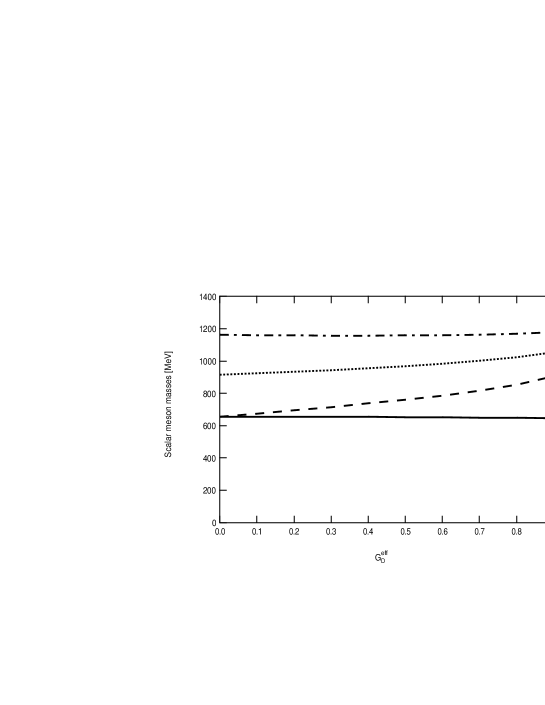
Figure 3.1: The calculated scalar meson masses as functions of the effective coupling constant $G_{D}^{\rm eff}$ of the $U_{A}(1)$ breaking KMT interaction. The solid, dashed, dotted and dash-dotted lines represent $m_{\sigma}$, $m_{a_{0}}$, $m_{K_{0}^{*}}$ and $m_{f_{0}}$, respectively.

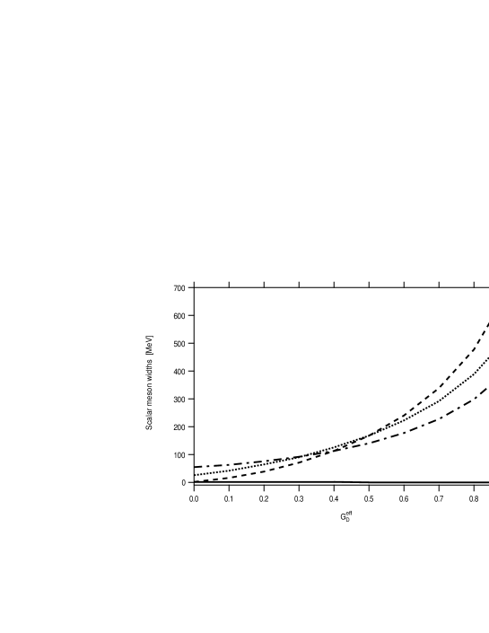
Figure 3.2: The calculated $q\mbox{$\bar{q}$}$ decay widths of the scalar mesons as functions of the effective coupling constant $G_{D}^{\rm eff}$ of the $U_{A}(1)$ breaking KMT interaction. The solid, dashed, dotted and dash-dotted lines represent $m_{\sigma}$, $m_{a_{0}}$, $m_{K_{0}^{*}}$ and $m_{f_{0}}$, respectively.

When $G_{D}^{\rm eff}$ is zero, our lagrangian does not cause the flavor mixing and therefore the ideal mixing is achieved. The $\sigma$ is purely $u\bar{u}+d\bar{d}$, which corresponds to $\theta=-54.7^{\circ}$, and is degenerate to the $a_{0}$ in this limit. When one increases the strength of the $U_{A}(1)$ breaking KMT interaction, the $q\mbox{$\bar{q}$}$ attraction in $\sigma$ increases and $\sigma$ state moves from the ideal mixing state toward the flavor singlet state. It means that the strange quark component of $\sigma$ increases as $G_{D}^{\rm eff}$ becomes bigger. Since the increase of the attractive force compensates with the increase of the strange quark component, $m_{\sigma}$ is almost independent of the strength of the $U_{A}(1)$ breaking interaction. The $\mbox{$\bar{q}$}q$ decay width of the $\sigma$ meson is very small, i.e., less than 2 MeV and therefore we neglect it in our calculation of the mixing angle. At $G_{D}^{\rm eff}=0.7$, the calculated mixing angle is $\theta=-77.3^{\circ}$, corresponding to about 15% mixing of the strangeness component in $\sigma$.

Hatsuda and Kunihiro have discussed the masses and mixing angle of the isoscalar nonstrange ($\sigma_{NS}$) and strange ($\sigma_{S}$) scalar mesons using the similar model.[19] They have reported a rather small mixing between $\sigma_{NS}$ and $\sigma_{S}$. The reason of the difference between their result and our result is the strength of the $U_{A}(1)$ breaking KMT interaction. The strength of the $U_{A}(1)$ breaking KMT interaction used in the present study is much stronger than that used in their study. They have determined the strength from the $\eta^{\prime}$ mass, while we have fixed it from the radiative decays of $\eta$. Strong $U_{A}(1)$ breaking interaction suggests that the instanton liquid picture of the QCD vacuum.[3] In Ref. [19], they have discussed the origin of the difference of the mixing properties of the scalar mesons and pseudoscalar mesons. We agree with their qualitative discussion, namely, the flavor mixing between $\sigma$ and $f_{0}$ is weaker than that between $\eta$ and $\eta^{\prime}$. Shakin has also pointed out that the KMT interaction mixes the $\sigma_{NS}$ and $\sigma_{S}$, while he assigned the lowest $I=0$ $q\mbox{$\bar{q}$}$ state to $f_{0}(980)$. [20]

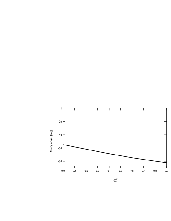
Figure 3.3: The calculated mixing angle of the $\sigma$ meson as a function of the effective coupling constant $G_{D}^{\rm eff}$ of the $U_{A}(1)$ breaking KMT interaction.

Let us turn to the discussion of the $a_{0}$ and $K_{0}^{*}$ mesons. As shown in Fig. 3.1, both $m_{a_{0}}$ and $m_{K_{0}^{*}}$ increase as $G_{D}^{\rm eff}$ increases. The slope for $m_{a_{0}}$ is steeper than that for $m_{K_{0}^{*}}$, which is consistent with the simple argument based on the form of the effective interaction Eq. (3.41). At $G_{D}^{\rm eff}=0.7$, the calculated masses are $m_{a_{0}}=816$ MeV and $m_{K_{0}^{*}}=1002$ MeV, therefore the $U_{A}(1)$ breaking interaction pushes up the $a_{0}$ and $K_{0}^{*}$ masses about 161 MeV and 88 MeV, respectively. Although the effect of the $U_{A}(1)$ breaking interaction on the $K_{0}^{*}$ meson is smaller than that on the $a_{0}$ meson, our numerical results show that it is not enough to support the existence of the light $\kappa$ state.

As for the $f_{0}$ meson, we have shown our results in Figs. 3.1 and 3.2. At $G_{D}^{\rm eff}=0$, the $f_{0}$ state is expected to be pure $s\mbox{$\bar{s}$}$ state in our model. Because of the $q\mbox{$\bar{q}$}$ decay width, we cannot calculate the mixing angle for $f_{0}$. The calculated mass of the $f_{0}$ meson at $G_{D}^{\rm eff}=0$ is $m_{f_{0}}=1.163$ GeV which is above the $s\mbox{$\bar{s}$}$ threshold $2M_{s}=1.113$ GeV. As shown in Ref. [21], the symmetry breaking effect by the current quark mass term pushes up the scalar meson mass above the $q\mbox{$\bar{q}$}$ threshold and the following relation is obtained by using the bosonization technique with the lowest order derivative expansion in the NJL model.

$$\left(m_{\rm scalar\,meson}^{2}-({q\bar{q}\,{\rm threshold\,energy})}^{2}\right)\propto m_{\rm current\,quark}$$ (3.43)

Our results at $G_{D}^{\rm eff}=0$ are $m_{a_{0}}^{2}-4M_{u}^{2}=0.008$ GeV², $m_{K_{0}^{*}}^{2}-(M_{u}+M_{s})^{2}=0.060$ GeV² and $m_{f_{0}}^{2}-4M_{s}^{2}=0.115$ GeV², respectively. The above simple mass relation therefore holds in our case too. Fig. 3.1 shows that the $f_{0}$ meson mass is almost independent of the strength of the KMT interaction. The situation is just opposite to the $\sigma$ case, i.e., the increase of the repulsive force by the KMT interaction compensates with the decrease of the strange quark component of the $f_{0}$ meson when one increases the strength of the KMT interaction.

It should be noted here that in the $SU_{L}(3)\times SU_{R}(3)$ version of linear sigma model, not only the three-meson flavor determinant term but also the chiral invariant four-meson terms give rise to the $\sigma-a_{0}$ mass difference. [22, 9] We note that the extended NJL model does not give such type of interaction.

Chapter 4 Formulation of the Improved Ladder Approximation Approach

In this chapter, we present the formulation of the Improved Ladder Approximation (ILA) of QCD. The approximation is applied to the Schwinger-Dyson (SD) equation for the quark propagator and to the Bethe-Salpeter (BS) equation for the pseudoscalar and scalar meson.

4.1 Lagrangian

The ladder approximation is the lowest order in the perturbation theory for the interaction kernels employed in this approximation may not be valid except for a heavy quark systems, where the coupling constant is small for this approximation. It, however, can be improved at low mass region by including a certain set of higher-order diagrams which bring the running coupling constant, $\alpha_{S}(p^{2})$.

In the present study we employ the following Lagrangian density the ILA of QCD,

$${\cal L}[\psi,\bar{\psi}]=\bar{\psi}(i\partial\!\!\!/-m_{0})\psi+{\cal L}_{\rm GE}[\psi,\bar{\psi}]+{\cal L}_{\rm KMT}[\psi,\bar{\psi}]$$ (4.1)

$$\psi=(u,d,s)^{T}.$$ (4.2)

In (4.1), $m_{0}$ denotes the bare quark mass matrix $m_{0}=\mbox{diag}(m_{q},m_{q},m_{s})$ where we assume the isospin invariance. ${\cal L}_{\rm GE}$ denotes the gluon exchange interaction

$${\cal L}_{\rm GE}[\psi,\bar{\psi}]= -\frac{1}{2}\int_{pp^{\prime}qq^{\prime}}{\cal K}^{mm^{\prime},nn^{\prime}}(p,p^{\prime},q,q^{\prime})$$ (4.3)

$$\qquad\qquad\times\bar{\psi}_{m}(p)\psi_{m^{\prime}}(p^{\prime})\bar{\psi}_{n}(q)\psi_{n^{\prime}}(q^{\prime})e^{-i(p+p^{\prime}+q+q^{\prime})x}$$

where

$${\cal K}^{mm^{\prime},nn^{\prime}}(p,p^{\prime},q,q^{\prime})=i\bar{g}^{2}D^{\mu\nu}\left(\frac{p+p^{\prime}}{2}-\frac{q+q^{\prime}}{2}\right)(\gamma_{\mu}T^{a})^{mm^{\prime}}(\gamma_{\nu}T^{a})^{nn^{\prime}}.$$ (4.4)

To reduce the expressions we use an abbreviation $\int_{p}{(2\pi)^{4}}$ through this chapter. The indeces $m,n,\cdots$ represent the components of the color, flavor and Dirac space. In the gluon propagator we employ the Landau gauge,

$$iD^{\mu\nu}(k)=\left(g^{\mu\nu}-\frac{k^{\mu}k^{\nu}}{k^{2}}\right)\frac{-1}{k^{2}}$$ (4.5)

and the Higashijima-Miransky type running coupling constant $\bar{g}^{2}$ defined as follows.

$$\bar{g}^{2}(p^{2}_{E},q^{2}_{E})=\theta(p^{2}_{E}-q^{2}_{E})g^{2}(p^{2}_{E})+\theta(q^{2}_{E}-p^{2}_{E})g^{2}(q^{2}_{E})$$ (4.6)

with

$$g^{2}(p_{E}^{2})=\left\{\begin{array}[]{ll}\frac{1}{\beta_{0}}\frac{1}{1+t}\mbox{for \quad}t_{\rm IF}\leq t\\ &\\ \frac{1}{2\beta_{0}}\frac{1}{(1+t_{\rm IF})^{2}}\left[3t_{\rm IF}-t_{0}+2-\frac{(t-t_{0})^{2}}{t_{\rm IF}-t_{0}}\right]&\mbox{for}\quad t_{0}\leq t\leq t_{\rm IF}\\ &\\ \frac{1}{2\beta_{0}}\frac{3t_{\rm IF}-t_{0}+2}{(1+t_{\rm IF})^{2}}&\mbox{for}\quad t\leq t_{0}\\ \end{array}\right.$$ (4.12)

$$t=\ln\frac{p_{E}^{2}}{\Lambda_{\rm QCD}^{2}}-1$$ (4.13)

$$\beta_{0}=\frac{1}{(4\pi)^{2}}\frac{11N_{C}-2N_{f}}{3}$$ (4.14)

Here, $p_{E}$ and $q_{E}$ denote the Euclidian momenta defined by

$$p=(p_{0},\vec{p})\quad \to \quad p_{E}=(ip_{4},\vec{p})$$ (4.15)

$$p^{2}=p_{0}^{2}-\vec{p}^{2}\quad \to \quad p^{2}_{E}=-p^{2}=\vec{p}^{2}+p_{o}^{2}$$ (4.16)

In eq.(4.12) the infrared cut-off $t_{\rm IF}$ is introduced. Above $t_{\rm IF}$ $g^{2}(p_{E}^{2})$ develops according to the one loop solution of the QCD renormalization group equation, while below $t_{0}$, $g^{2}(p_{E}^{2})$ is kept constant. These two regions are connected by a quadratic polynomial so that $g^{2}(p_{E}^{2})$ becomes a smooth function. Here $N_{C}$ and $N_{f}$ are the number of colors and active flavors respectively. We use $N_{C}=N_{f}=3$ in this study. The behavior of the running coupling constant is shown in the Fig. 4.1 together with the one-loop QCD running coupling constant for $\Lambda_{\rm QCD}=600[\mbox{MeV}]$.

Figure 4.1: The running coupling constant of the QCD and the ILA

${\cal L}_{\rm KMT}$ is the Kobayashi-Maskawa-’t Hooft (KMT) interaction given by

$${\cal L}_{\rm KMT}= -\frac{1}{3}G_{D}\epsilon^{f_{1}f_{2}f_{3}}\epsilon^{g_{1}g_{2}g_{3}}\bar{w}(\partial_{x_{1}};\partial_{y_{1}};\partial_{x_{2}};\partial_{y_{2}};\partial_{x_{3}};\partial_{y_{3}})$$ (4.17)

$$\times\left\{[\bar{\psi}_{g_{1}}(x_{1})\psi_{f_{1}}(y_{1})][\bar{\psi}_{g_{2}}(x_{2})\psi_{f_{2}}(y_{2})][\bar{\psi}_{g_{3}}(x_{3})\psi_{f_{3}}(y_{3})]\right.$$

$$+3\left.[\bar{\psi}_{g_{1}}(x_{1})\psi_{f_{1}}(y_{1})][\bar{\psi}_{g_{2}}(x_{2})\gamma_{5}\psi_{f_{2}}(y_{2})][\bar{\psi}_{g_{3}}(x_{3})\gamma_{5}\psi_{f_{3}}(y_{3})]\right\}\Bigg{|}_{*}$$

where $f_{1},g_{1},\cdots$ are flavor indices, $\epsilon$ denotes the antisymmetric tensor with $\epsilon^{uds}=1$ and the symbol $*$ at the end of the equation means to take the limit $x_{1},x_{2},\cdots\to x$ after all derivatives are operated. This interaction causes the $U_{A}(1)$ symmetry breaking and also flavor mixing.

We introduce a weight function $\bar{w}$ which is necessary so that the KMT interaction is turned off at the high energy region. Then the asymptotic behavior of the ILA are kept. We use the following Gaussian form

$$\bar{w}(\partial_{x_{1}};\partial_{y_{1}};\partial_{x_{2}};\partial_{y_{2}};\partial_{x_{3}};\partial_{y_{3}})=\bar{w}\left(\frac{\partial^{2}_{x_{1}}+\partial^{2}_{x_{2}}+\partial^{2}_{x_{3}}+\partial^{2}_{y_{1}}+\partial^{2}_{y_{2}}+\partial^{2}_{y_{3}}}{2}\right)$$ (4.18)

$$w(\mu^{2})=\exp(-\kappa\mu^{2})$$ (4.19)

This weight function is convenient for numerical calculations as it is factorized as

$$w(-p^{2}-q^{2})=w(-p^{2})w(-q^{2}).$$ (4.20)

The parameter $\kappa$ is taken as

$$\kappa=0.7[\mbox{GeV}^{-2}].$$ (4.21)

This value corresponds to the form factor of the instanton of the average size $\rho$, about $1/3$[fm]. The instanton form factor,

$$\frac{1}{x_{E}^{2}+\rho^{2}}\propto 1-\frac{x^{2}_{E}}{\rho^{2}}+\cdots$$ (4.22)

can be identified for small $x_{E}^{2}$ with the Fourier transformation of the weight function

$$\mbox{F.T.}w(q^{2}_{E})=C\exp\left(-\frac{x^{2}_{E}}{4\kappa}\right)\propto 1-\frac{x^{2}_{E}}{4\kappa}+\cdots$$ (4.23)

with

$$4\kappa=\rho^{2}.$$ (4.24)

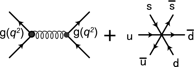
Figure 4.2: The interactions of the ILA.

Finally we introduce the ultraviolet momentum cutoff $\Lambda_{\rm UV}$, which is necessary to regularize loop integrals in the ILA approach. It is useful to introduce the cutoff function

$$\frac{1}{f(p^{2})}=\left\{\begin{array}[]{cc}1&p^{2}<\Lambda_{\rm UV}^{2}\\ 0&p^{2}>\Lambda_{\rm UV}^{2}\end{array}\right.$$ (4.27)

By adding it in the kinetic term as

$$\bar{\psi}f(\partial^{2})(i\partial\!\!\!/-m_{0})\psi$$ (4.28)

all integrals are regularized. We choose a very large $\Lambda_{\rm UV}$ ($\sim 100[\mbox{GeV}]$) so that the results are not sensitive to the value of $\Lambda_{\rm UV}$.

It should be noted that because the cut off function, f and w, depend on the momentum, the Noether currents are modified from the bare QCD currents.

4.2 Renormalization of Quark Masses

In our approach, the parameters of the Lagrangian are renormalized at the cutoff scale $\Lambda_{\rm UV}$. Since the $\Lambda_{\rm UV}$ should be taken enough large, it may not be appropriate to fix the quark mass at such high energy. Instead of the quark mass ${m_{q}}_{0}$, ${m_{s}}_{0}$ at the scale $\Lambda_{\rm UV}$, we choose renormalized the quark mass at the momentum scale $\mu=2[\mbox{GeV}]$ as ${m_{q}}_{R}=5[\mbox{MeV}]$ and ${m_{s}}_{R}=100[\mbox{MeV}]$ and calculate the ${m_{q}}_{0}$ and ${m_{s}}_{0}$ in the following way.

The renormalization constants $Z_{m_{q}}$ and $Z_{m_{s}}$ are defined by

$$m_{q}=Z_{m_{q}}^{-1}{m_{q}}_{R},\quad m_{s}=Z_{m_{s}}^{-1}{m_{s}}_{R}.$$ (4.29)

We take the renormalization condition as

$$\frac{\partial B_{q}(\mu^{2})}{\partial{m_{q}}_{R}}\Bigg{|}_{m_{qR}}=0$$ (4.30)

$$\frac{\partial B_{s}(\mu^{2})}{\partial{m_{s}}_{R}}\Bigg{|}_{m_{sR}}=0.$$ (4.31)

We define the quark condensate as follows

$$<:\bar{\psi}(0)\psi(0):>=-\int_{p}\mbox{Tr}[S_{F}^{\rm Full}(p)]+\int_{p}Tr[S_{F}^{\rm bare}]$$ (4.32)

where

$$\int_{p}\mbox{Tr}[S_{F}^{\rm Full}(p)]=N_{C}\int_{p}\frac{4iB(p^{2})}{p^{2}-B^{2}(p^{2})}$$ (4.33)

$$\int_{p}\mbox{Tr}[S_{F}^{\rm bare}(p)]=N_{C}\int_{p}\frac{4i\frac{\partial B}{\partial m_{R}}m_{R}}{p^{2}-\left(\frac{\partial B}{\partial m_{R}}m_{R}\right)^{2}}$$ (4.34)

4.3 Effective Action

To derive the Schwinger-Dyson (SD) equation and the Bethe-Salpeter (BS) equation, we use the Cornwall-Jackiw-Tomboulis (CJT) effective action formulation [29].

The CJT effective action is defined as

$$\Gamma[S_{F}]=i\mbox{Tr}\mbox{Ln}[S_{F}]-i\mbox{Tr}[S_{0}^{-1}S_{F}]+\Gamma_{\rm loop}[S_{F}]$$ (4.35)

The last term of Eq.$(\ref{CJTaction})$ is the residual term, and is given by the sum of all the Feynman amplitudes of corresponding to the two particle irreducible vacuum diagrams with two ore more loops. In these amplitudes, quark propagator is substituted by the full propagator

$$S_{F}(x,y)=\langle 0|T\psi(x)\bar{\psi}(y)|0\rangle.$$ (4.36)

In this study, we employ the lowest loop order and the leading $1/N_{C}$ contribution for the $\Gamma_{\rm loop}[S_{F}]$. Then the CJT action becomes

$$\Gamma[S_{F}]=i\mbox{Tr}\mbox{Ln}[S_{F}]-i\mbox{Tr}[S_{0}^{-1}S_{F}]+\Gamma_{\rm GE}[S_{F}]+\Gamma_{\rm KMT}[S_{F}]$$ (4.37)

where

$$\Gamma_{\rm GE}[S_{F}]= -\frac{1}{2}\int d^{4}x{\cal K}^{m_{1}m_{2},n_{1}n_{2}}(i\partial_{x_{1}},i\partial_{x_{2}};i\partial_{y_{1}},i\partial_{y_{2}})$$ (4.38)

$$\times\left({S_{F}}_{m_{2}m_{1}}(x_{2},x_{1}){S_{F}}_{n_{2}n_{1}}(y_{2},y_{1})-{S_{F}}_{m_{2}n_{1}}(x_{2},y_{1}){S_{F}}_{n_{2}m_{1}}(y_{2},x_{1})\right)\Bigg{|}_{*}$$

$$\Gamma_{\rm KMT}[S_{F}]= -\frac{G_{D}}{3}\int d^{4}x\epsilon^{f_{1}f_{2}f_{3}g_{1}g_{2}g_{3}}w\left(\frac{\partial^{2}_{x_{1}}+\partial^{2}_{y_{1}}+\partial^{2}_{x_{2}}+\partial^{2}_{y_{2}}+\partial^{2}_{x_{3}}+\partial^{2}_{y_{3}}}{2}\right)$$

$$\times\left(-\mbox{tr}^{\rm(DC)}[{S_{F}}_{f_{1}g_{1}}(y_{1},x_{1})]\mbox{tr}^{\rm(DC)}[{S_{F}}_{f_{2}g_{2}}(y_{2},x_{2})]\mbox{tr}^{\rm(DC)}[{S_{F}}_{f_{3}g_{3}}(y_{3},x_{3})]\right.$$

$$\qquad\left.-3\mbox{tr}^{\rm(DC)}[{S_{F}}_{f_{1}g_{1}}(y_{1},x_{1})]\mbox{tr}^{\rm(DC)}[\gamma_{5}{S_{F}}_{f_{2}g_{2}}(y_{2},x_{2})]\mbox{tr}^{\rm(DC)}[\gamma_{5}{S_{F}}_{f_{3}g_{3}}(y_{3},x_{3})]\right)\Bigg{|}_{*}.$$

It should be noted that the global $SU_{L}(3)\times SU_{R}(3)$ symmetry is preserved within this approximation if the quark masses $m_{q}$ and $m_{s}$ vanish.

In fact, the total effective action $\Gamma[S_{F}]$ is invariant under the infinitesimal global chiral transformation

$$S_{F}(x,y)\to\left(1+i\gamma_{5}\frac{\lambda^{a}}{2}\theta^{a}\right)S_{F}(x,y)\left(1+i\gamma_{5}\frac{\lambda^{a}}{2}\theta^{a}\right),$$ (4.40)

except for the quark mass term.

From this truncated effective action, the rainbow SD equation and the ladder BS equation are derived consistently.

4.4 Schwinger Dyson equation

The Schwinger-Dyson equation is derived by the stability condition of the CJT action

$$\frac{\delta\Gamma[S_{F}]}{\delta S_{F}(x,y)}=0.$$ (4.41)

Introducing the regularized propagators

$$S_{F}^{R}(q)=f(q^{2})S_{F}(q)$$ (4.42)

$$S_{0}^{R}(q)=f(q^{2})S_{0}(q),$$ (4.43)

the SD equation in the momentum space becomes

$$i{S_{F}^{R}}^{-1}(q)-i{S_{0}^{R}}^{-1}(q) = -\frac{C_{F}}{f(-q^{2})}\int_{p}\frac{1}{f(-p^{2})}\bar{g}^{2}(-q^{2},-p^{2})iD^{\mu\nu}(p-q)\gamma_{\mu}S_{F}(p)\gamma_{\nu}$$ (4.44)

$$-G_{D}\mbox{{\boldmath$1$}}_{C}\mbox{{\boldmath$1$}}_{f}\epsilon^{gf_{1}f_{2}}\epsilon^{fg_{1}g_{2}}\int_{p,k}\frac{1}{f(-p^{2})f(-k^{2})}w(-q^{2}-p^{2}-k^{2})$$

$$\qquad\qquad\qquad\times\mbox{tr}^{\rm(DC)}[{S_{F}^{R}(p)}_{g_{1}f_{1}}]\mbox{tr}^{\rm(DC)}[{S_{F}^{R}(k)}_{g_{2}f_{2}}]$$

with the coefficient from the color space,

$$C_{F}=\frac{\mbox{tr}[T^{a}T^{a}]}{N_{C}}=\frac{N_{C}^{2}-1}{2N_{C}}.$$ (4.45)

This equation is shown diagrammatically in Fig.$(\ref{FIG_SDeq})$.

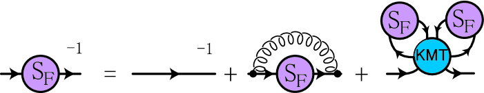
Figure 4.3: The SD equation

Generally the quark propagator is parametrized as

$$S_{F}^{R}(q)=\frac{i}{q\!\!\!/A(q^{2})-B(q^{2})}.$$ (4.46)

In the Landau gauge, it can be shown that the solution satisfies $A(-q_{E}^{2})=1$. Then the SD equation becomes the integral equation only of the mass function $B(q^{2})$ and reads

$$B_{q}(-q^{2})= m_{q}+\frac{3C_{F}}{16\pi^{2}}\int^{\Lambda_{\rm UV}^{2}}_{0}dk^{2}\bar{g}^{2}(q^{2},k^{2})\left\{\theta(k^{2}-q^{2})+\frac{k^{2}}{q^{2}}\theta(q^{2}-k^{2})\right\}\frac{B_{q}(-k^{2})}{k^{2}+B_{q}(-k^{2})}$$

$$+\frac{G_{D}N_{C}^{2}w(q^{2})}{8\pi^{4}}\int^{\Lambda_{\rm UV}^{2}}_{0}dk^{2}w(k^{2})\frac{k^{2}B_{q}(-k^{2})}{k^{2}+B_{q}(-k^{2})}\int^{\Lambda_{\rm UV}^{2}}_{0}dl^{2}w(l^{2})\frac{l^{2}B_{s}(-l^{2})}{l^{2}+B_{s}(-l^{2})}$$

$$B_{s}(-q^{2})= m_{s}+\frac{3C_{F}}{16\pi^{2}}\int^{\Lambda_{\rm UV}^{2}}_{0}dk^{2}\bar{g}^{2}(q^{2},k^{2})\left\{\theta(k^{2}-q^{2})+\frac{k^{2}}{q^{2}}\theta(q^{2}-k^{2})\right\}\frac{B_{s}(-k^{2})}{k^{2}+B_{s}(-k^{2})}$$

$$+\frac{G_{D}N_{C}^{2}w(q^{2})}{8\pi^{4}}\int^{\Lambda_{\rm UV}^{2}}_{0}dk^{2}w(k^{2})\frac{k^{2}B_{q}(-k^{2})}{k^{2}+B_{q}(-k^{2})}\int^{\Lambda_{\rm UV}^{2}}_{0}dl^{2}w(l^{2})\frac{l^{2}B_{q}(-l^{2})}{l^{2}+B_{q}(-l^{2})}.$$

4.5 Bethe-Salpeter equation

To treat the pseudoscalar mesons and the scalar meson as quark-antiquark bound state, we use the homogeneous Bethe-Salpeter equation. It is derived by

$$\frac{\delta^{2}\Gamma[S_{F}]}{\delta{S_{F}}_{mn}(x,y)\delta{S_{F}}_{m^{\prime}n^{\prime}}(y^{\prime},x^{\prime})}\chi_{n^{\prime},m^{\prime}}(y^{\prime},x^{\prime};P_{B})=0$$ (4.49)

where

$$\chi_{n^{\prime},m^{\prime}}(y^{\prime},x^{\prime};P_{B})=\langle 0|T\psi_{n^{\prime}}(y^{\prime})\bar{\psi}_{m^{\prime}}(x^{\prime})|\mbox{{\boldmath$P$}}\rangle$$ (4.50)

denotes the BS amplitude. The normalization condition is taken as

$$\langle\mbox{{\boldmath$P$}}_{B}|\mbox{{\boldmath$P^{\prime}_{B}$}}\rangle=(2\pi)^{3}2{P_{B}}_{0}\delta^{3}(\mbox{{\boldmath$P$}}_{B}-\mbox{{\boldmath$P$}}^{\prime}_{B})$$ (4.51)

and $P_{B}=\sqrt{M_{B}^{2}+\mbox{{\boldmath$P$}}_{B}^{2}}$ where $\mbox{{\boldmath$P$}}_{B}$ is the on-shell momentum of the meson.

Introducing the regularized BS amplitude by

$$\chi^{R}_{n^{\prime},m^{\prime}}(q;P_{B})=f(-q_{+}^{2})\chi_{n^{\prime},m^{\prime}}(q;P_{B})f(-q_{-}^{2})$$ (4.52)

$$q_{+}=q+\frac{P_{B}}{2},\qquad q_{-}=q-\frac{P_{B}}{2}$$ (4.53)

the BS equation in momentum space becomes

$$S_{F}^{R^{-1}}(q_{+})\chi^{R}(q;P)S_{F}^{R^{-1}}(q_{-})$$

$$=-iC_{F}\int_{k}\frac{1}{f(-k_{+}^{2})f(-k_{-}^{2})}\bar{g}^{2}(-q^{2},-k^{2})iD^{\mu\nu}(q-k)\gamma_{\mu}\chi^{R}(k;P)\gamma_{\nu}$$

$$-2iG_{D}\epsilon^{ghf^{\prime}}\epsilon^{fh^{\prime}g^{\prime}}\mbox{{\boldmath$1$}}_{C}\int_{p,k}\frac{1}{f(-p^{2})f(-k_{+}^{2})f(-k_{-}^{2})}w\left(-p^{2}-q^{2}-k^{2}-\frac{P_{B}^{2}}{2}\right)$$

$$\times\mbox{tr}^{(DC)}[{S_{F}^{R}}_{h^{\prime}h}(p)]\left\{(\gamma_{5})\mbox{tr}^{(DC)}[\gamma_{5}\chi^{R}_{g^{\prime}f^{\prime}}(k;P_{B})]+(1)\mbox{tr}^{(DC)}[\chi^{R}_{g^{\prime}f^{\prime}}(k;P_{B})]\right\}$$ (4.54)

which is shown diagrammatically in Fig.(4.4).

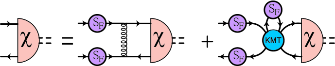
Figure 4.4: The BS equation

For the pion, the BS amplitude can be written in terms of four scalar amplitudes as in Ref.[18],

$$\chi^{R}_{nm}(k;P)=\mbox{{\boldmath$1$}}_{C}\frac{\lambda^{a}}{2}\left(\phi_{S}(k;P)+\phi_{P}(k;P)k\!\!\!/+\phi_{Q}(k;P)P\!\!\!\!/+\phi_{T}(k;P)\frac{1}{2}(P\!\!\!\!/k\!\!\!/-k\!\!\!/P\!\!\!\!/)\right)\gamma_{5}$$ (4.55)

where $\lambda^{a}$ denotes the flavor structure of the pion state. The neutral pion, for instance, is given by $a=3$

$$\lambda^{3}=\left(\begin{array}[]{ccc}1&0&0\\ 0&-1&0\\ 0&0&0\\ \end{array}\right)$$ (4.59)

On the other hand, for the $\eta$ and $\eta^{\prime}$ mesons, the BS amplitudes are written in terms of eight scalar amplitudes,

$$\chi^{R}_{nm}= \mbox{{\boldmath$1$}}_{C}\frac{\lambda^{q}}{2}\left(\phi^{q}_{S}(k;P)+\phi^{q}_{P}(k;P)k\!\!\!/+\phi^{q}_{Q}(k;P)P\!\!\!\!/+\phi^{q}_{T}(k;P)\frac{1}{2}(P\!\!\!\!/k\!\!\!/-k\!\!\!/P\!\!\!\!/)\right)\gamma_{5}$$ (4.60)

$$+ \mbox{{\boldmath$1$}}_{C}\frac{\lambda^{s}}{2}\left(\phi^{s}_{S}(k;P)+\phi^{s}_{P}(k;P)k\!\!\!/+\phi^{s}_{Q}(k;P)P\!\!\!\!/+\phi^{s}_{T}(k;P)\frac{1}{2}(P\!\!\!\!/k\!\!\!/-k\!\!\!/P\!\!\!\!/)\right)\gamma_{5}$$

where the flavor matrices $\lambda^{q}$ and $\lambda^{s}$ are defined by

$$\lambda^{q}=\left(\begin{array}[]{ccc}1&0&0\\ 0&1&0\\ 0&0&0\\ \end{array}\right),\qquad\lambda^{s}=\left(\begin{array}[]{ccc}0&0&0\\ 0&0&0\\ 0&0&\sqrt{2}\\ \end{array}\right).$$ (4.67)

Because of the flavor mixing effects caused by the KMT interaction, the q and s components of the BS amplitude are mixed. We identify the ground state solution with the $\eta$ meson state and the first excited state with the $\eta^{\prime}$ meson state. The explicit form of the BS equation is given in the appendix.

Similarly the pseudoscalar mesons, the BS amplitude of the scalar meson is parametrized as

$$\chi^{R}_{nm}(k;P)=\mbox{{\boldmath$1$}}_{C}\frac{\lambda^{a}}{2}\left(\phi_{S}(k;P)+\phi_{P}(k;P)k\!\!\!/+\phi_{Q}(k;P)P\!\!\!\!/+\phi_{T}(k;P)\frac{1}{2}(P\!\!\!\!/k\!\!\!/-k\!\!\!/P\!\!\!\!/)\right)$$ (4.68)

for $a_{0}$ and

$$\chi^{R}_{nm}= \mbox{{\boldmath$1$}}_{C}\frac{\lambda^{q}}{2}\left(\phi^{q}_{S}(k;P)+\phi^{q}_{P}(k;P)k\!\!\!/+\phi^{q}_{Q}(k;P)P\!\!\!\!/+\phi^{q}_{T}(k;P)\frac{1}{2}(P\!\!\!\!/k\!\!\!/-k\!\!\!/P\!\!\!\!/)\right)$$ (4.69)

$$+ \mbox{{\boldmath$1$}}_{C}\frac{\lambda^{s}}{2}\left(\phi^{s}_{S}(k;P)+\phi^{s}_{P}(k;P)k\!\!\!/+\phi^{s}_{Q}(k;P)P\!\!\!\!/+\phi^{s}_{T}(k;P)\frac{1}{2}(P\!\!\!\!/k\!\!\!/-k\!\!\!/P\!\!\!\!/)\right)$$

for $\sigma$ or $f_{0}$, respectively.

In the numerical computation, we treat the BS equation in the Euclidean momentum region. Then the physical solution, which corresponds to negative $P_{E}^{2}$, is obtained only by extrapolation from the $P_{E}^{2}>0$ region. It can be done in the following way. First, we rewrite the Euclidean BS equation in the form

$$\phi_{A}(q;P_{E})=\int_{k_{E}}M_{AB}(q_{E};k_{E};P_{E})\phi_{B}(k;P_{E})$$ (4.70)

where $\phi_{A}$ and $\phi_{B}$ denotes the set of amplitude. This equation should not have solution at $P_{E}^{2}>0$ because, if it exists, it is a tachyon solution. Therefore we instead solve the eigenvalue equation

$$\lambda(P_{E}^{2})\phi_{A}(q_{E};P_{E})=\int_{k}M_{AB}(q_{E};k_{E};P_{E})\phi_{B}(k_{E};P_{E})$$ (4.71)

for a fixed $P_{E}^{2}>0$. Then we extrapolate the eigenvalue to $P_{E}^{2}<0$ as a function of $P^{2}_{E}$ and search for the on-shell point $\lambda(-M_{B}^{2})=1$. We employ the quadratic function of $P_{E}^{2}$ for the extrapolation. We also check the results using the PCAC relation.

4.6 Normalization and Decay Constants

4.6.1 Normalization

In order to obtain the decay constants of the pseudoscalar mesons, it is necessary to normalize the BS amplitude derived from the inhomogeneous BS equation. The normalization condition of the BS amplitude is given by

$$i\int_{q}\frac{1}{f(-q_{+}^{2})f(-q_{-}^{2})}\chi^{R}_{n_{1}m_{1}}(q;P)\bar{\chi}^{R}_{m_{2}n_{2}}(q;P)P^{\mu}\frac{\partial}{\partial P^{\mu}}\left\{{S_{F}^{R}}_{n_{2}n_{1}}^{-1}(q_{+}){S_{F}^{R}}_{m_{1}m_{2}}^{-1}(q_{-})\right\}=-2P^{2}.$$ (4.72)

The explicit form of this equation is shown in the appendix.

4.6.2 Calculation of the Decay Constant

Using the normalized BS amplitude, the decay constants of the pseudoscalar mesons are obtained by

$$f_{B}=\frac{1}{P_{B}^{2}}\int_{q} \frac{1}{f(-q_{-}^{2})f(-q_{+}^{2})}$$

$$\times\mbox{Tr}\left[\bar{\chi}^{R}(q;P_{B})\left\{i\gamma_{5}\frac{\lambda^{\alpha}}{2}\left(\frac{f(-q_{-}^{2})+f(-q_{+}^{2})}{2}P\!\!\!\!/+(f(-q_{+}^{2})-f(-q_{-}^{2}))q\!\!\!/\right)\right.\right.$$

$$\left.\left.\qquad\quad+E^{\alpha}(q;P)+F^{\alpha}(q;P)\right\}\right]$$

$$E^{\alpha}_{mn}(q;P)=\int_{k} \left[\left\{K^{n^{\prime}nmm^{\prime}}_{(-k,q-\frac{P}{2},-q-\frac{P}{2},k+P)}-K^{n^{\prime}nmm^{\prime}}_{(-k,q-\frac{P}{2},-q+\frac{P}{2},k)}\right\}\left(i\gamma_{5}\frac{\lambda^{\alpha}}{2}S_{F}(k)\right)_{m^{\prime}n^{\prime}}\right.$$

$$+\left.\left\{K^{n^{\prime}nmm^{\prime}}_{(-k+P,q-\frac{P}{2},-q-\frac{P}{2},k)}-K^{n^{\prime}nmm^{\prime}}_{(-k,q+\frac{P}{2},-q-\frac{P}{2},k)}\right\}\left(S_{F}(k)i\gamma_{5}\frac{\lambda^{\alpha}}{2}\right)_{m^{\prime}n^{\prime}}\right]$$

$$F^{\alpha}_{mn}(q;P) = -2G_{D}\gamma_{5}\mbox{{\boldmath$1$}}_{color}\int_{k,l}\frac{1}{f(-k^{2})f(-l^{2})}\mbox{tr}^{(DC)}[{S_{F}^{R}}_{g_{2}f_{2}}(k)]$$ (4.75)

$$\quad\times\left[\left\{w\left(-(q-\frac{P}{2})^{2}-k^{2}-l^{2}\right)-w\left(-q^{2}-\frac{3}{4}P^{2}-k^{2}-l^{2}+Pl\right)\right\}\right.$$

$$\quad\quad\times\epsilon^{ff_{2}f_{3}}\epsilon^{gg_{2}g_{3}}\mbox{tr}^{(DC)}\left[{S_{F}^{R}}(l)i\frac{\lambda^{\alpha}}{2}\right]_{g_{3}f_{3}}$$

$$\quad\quad+\left\{w\left(-(q+\frac{P}{2})^{2}-k^{2}-l^{2}\right)-w\left(-q^{2}-\frac{3}{4}P^{2}-k^{2}-l^{2}-Pl\right)\right\}$$

$$\quad\quad\left.\times\epsilon^{ff_{2}f_{3}}\epsilon^{gg_{2}g_{3}}\mbox{tr}^{(DC)}\left[i\frac{\lambda^{\alpha}}{2}{S_{F}^{R}}(l)\right]_{g_{3}f_{3}}\right]$$

The terms $E^{\alpha}(q;P)$ and $F^{\alpha}(q;P)$ represent the corrections to the Noether axialvector current due to the momentum dependencies interaction.

For the $\eta$ and $\eta^{\prime}$ mesons, the flavor structure of the BS amplitude depends on the relative and total momenta in general. Therefore we can not fix $\lambda^{\alpha}$ in the definition of the decay constant from the flavor structure of the BS amplitude. Instead we only consider the decay constants associated with the octet and singlet axialvector currents for the $\eta$, $\eta^{\prime}$ mesons, i.e., we define and calculate $f_{8}^{\eta}$, $f_{0}^{\eta}$ ,$f_{8}^{\eta^{\prime}}$ and $f_{0}^{\eta^{\prime}}$.

Since the BS equation is homogeneous, the overall sign of the BS amplitude, and therefore the decay constants, cannot be determined. We choose the sign as

$$\left\{\begin{array}[]{l}f^{8}_{\eta}>0\qquad\mbox{for}\qquad\eta\\ f^{0}_{\eta^{\prime}}>0\qquad\mbox{for}\qquad\eta^{\prime}\quad.\\ \end{array}\right.$$ (4.78)

4.7 PCAC relation

In our approach, there are eight axial-vector currents, $J_{5\mu}^{\alpha}(\alpha=1,\cdots,8)$ , which satisfy the PCAC relation

$$\partial^{\mu}J_{5\mu}^{\alpha}(x)=2\left[m_{0}J_{5}\right]^{\alpha}(x)$$ (4.79)

$$\left[m_{0}J_{5}\right]^{\alpha}(x)=\bar{\psi}i\gamma_{5}\frac{f(\stackrel{{\scriptstyle\leftarrow}}{{\partial^{2}}})m_{0}\lambda^{\alpha}+\lambda^{\alpha}m_{0}f(\partial^{2})}{4}\psi.$$ (4.80)

We take the matrix element of both the sides of eq. (4.79) between a meson state $\langle\mbox{{\boldmath$P$}}_{B}|$ and the vacuum $|0\rangle$ and obtain

$$-f_{B}^{\alpha}M_{B}^{2}=2[m_{0}{\cal E}_{B}^{\alpha}]$$ (4.81)

where $f_{B}^{\alpha}$ means the decay constant $f_{\pi},f_{8}^{\eta},f_{8}^{\eta^{\prime}}$. $[m_{0}{\cal E}_{B}^{\alpha}]$ is defined by

$$[m_{0}{\cal E}_{B}^{\alpha}]=\lim_{P\to P_{B}}i\int_{q}\frac{1}{2}\left(\frac{1}{f(-q_{-}^{2})}+\frac{1}{f(-q_{+}^{2})}\right)\mbox{tr}\left[\bar{\chi}^{R}(q;P)m_{0}\gamma_{5}\frac{\lambda^{\alpha}}{2}\right]$$ (4.82)

Since this relation must be kept on the mass shell, we can use this as a check of the obtained mass by using the extrapolation. We introduce the ratio R defined by

$$R^{\alpha}(P_{E}^{2})=\frac{f^{\alpha}_{B}(P_{E}^{2})P_{E}^{2}}{2[m_{0}{\cal E}_{B}]^{\alpha}(P_{E}^{2})}.$$ (4.83)

As this ratio should become unity at $P_{E}^{2}=-M_{B}^{2}$, the value of $R^{\alpha}(-M_{E}^{2})$ is a good measure of the accuracy of the calculation, especially the extrapolation from the $P_{E}^{2}>0$ region to $P_{E}^{2}=-M_{B}^{2}$ point.

Chapter 5 Results and Discussion

In this chapter, we show the numerical results and give the disscussion.

5.1 Parameters

In the present approach, there are eight input parameters: quark mass ${m_{q}}_{0}$ for the up and down quarks, the current quark mass ${m_{s}}_{0}$ for the strange quark, the scale parameter of QCD running coupling constant $\Lambda_{\rm QCD}$, the infrared cutoff $t_{\rm IF}$, the smoothness parameter $t_{0}$, the strength parameter of the KMT $G_{D}$, the parameter of the weight function of the KMT $\kappa$ and the ultraviolet cutoff $\Lambda_{\rm UV}$. We take the ultraviolet cutoff $\Lambda_{\rm UV}=100[\mbox{GeV}]$ and at such large value the physical observables do not depend on it. The quark masses ${m_{q}}_{0},{m_{s}}_{0}$ are chosen so that the renormalized masses at the momentum scale $\mu=2[\mbox{GeV}]$ become the ${m_{q}}_{R}=4.5[\mbox{MeV}]$ and ${m_{s}}_{R}=150[\mbox{MeV}]$, respectively. The $\kappa$ parameter is taken as $\kappa=0.7[\mbox{GeV}^{-2}]$, which corresponds to the instanton of the average size $1/3[{\rm fm}]$ as shown in Sec.[4.1]. The other parameters $\Lambda_{\rm QCD}$, $t_{\rm IF}$, $t_{0}$, $G_{D}$ are chosen as the pseudoscalar meson masses $M_{\pi}$, $M_{\eta}$, $M_{\eta^{\prime}}$ and the pion decay constant $f_{\pi}$ are fitted to the experimental values. The parameters we used are $\Lambda_{\rm QCD}=600[\mbox{MeV}]$, $t_{0}=-6.89$, $t_{\rm IF}=0.204$ and $G_{D}=75[\mbox{GeV}^{-5}]$.

The results of the calculation with these parameters are $M_{\pi}=136[\mbox{MeV}]$, $M_{\eta}=515[\mbox{MeV}]$, $M_{\eta^{\prime}}=982[\mbox{MeV}]$ and $f_{\pi}=95[\mbox{MeV}]$. These are in agreement with experimental values in less than $6\%$ of deviation. Table 5.1 summarizes all the values of the parameters.

Although $\Lambda_{\rm QCD}$ is somewhat larger than the standard value $\Lambda_{\rm QCD}=100\sim 300[\mbox{MeV}]$, a large $\Lambda_{\rm QCD}$ is necessary in the ILA to generate the desired dynamical chiral symmetry breaking (D$\chi$SB). It may indicate that the chiral symmetry breaking is not fully explained by the ladder approximation of the one gluon exchange with $U_{A}(1)$ breaking effect. If we take a strong KMT interaction, we may reduce $\Lambda_{\rm QCD}$, but then $\eta-\eta^{\prime}$ mass splitting becomes too large. As a result, we should choose a large $\Lambda_{\rm QCD}$ so that the D$\chi$SB is generated mainly by the gluon exchange interaction. Although the results of our calculation show that the contribution of the KMT interaction to the quark mass function and to the quark condensate is small ($\leq 10\%$), it gives significant effects on the mass spectrum and the mixing angle. Then this KMT interaction can be regarded to induce strong $U_{A}(1)$ breaking.

${m_{q}}_{R}(2[\mbox{GeV}])$	$4.5[\mbox{MeV}]$
${m_{s}}_{R}(2[\mbox{GeV}])$	$150[\mbox{MeV}]$
$\Lambda_{\rm QCD}$	$600[\mbox{MeV}]$
$t_{\rm IF}$	$0.204$
$t_{0}$	$-6.89$
$G_{D}$	$75[\mbox{GeV}^{-5}]$
$\kappa$	$0.7[\mbox{GeV}^{-2}]$
$\Lambda_{\rm UV}$	$100[\mbox{GeV}]$

             $M_{\pi}$ $136[\mbox{MeV}]$ $M_{\eta}$ $515[\mbox{MeV}]$ $M_{\eta^{\prime}}$ $982[\mbox{MeV}]$ $f_{\pi}$ $95[\mbox{MeV}]$

Table 5.1: The values of the the parameters in the ILA approach and the obtained observable quantities.

5.2 Solution of the SD equation

Let us now discuss the solutions of the SD equation. Our numerical results of the running quark masses are shown in Fig.5.1 and 5.2. The values of the quark condensates and mass function at $P_{E}^{2}=0$ are given in the Table 5.2.

Figure 5.1: $q_{E}^{2}$ dependences of the mass function of the q quark $B_{q}$ with $G_{D}=0,25,50,75,$ $100[\mbox{GeV}^{-5}]$

Figure 5.2: $q_{E}^{2}$ dependences of the mass function of the q quark $B_{s}$ with $G_{D}=0,25,50,75,$ $100[\mbox{GeV}^{-5}]$

$G_{D}[\mbox{GeV}^{5}]$	$B_{q}(0)[\mbox{GeV}]$	$B_{s}(0)[\mbox{GeV}]$	$-\langle\bar{q}q\rangle_{R}^{1/3}[\mbox{GeV}]$	$-\langle\bar{s}s\rangle_{R}^{1/3}[\mbox{GeV}]$
0	0.524	0.744	$0.225$	$0.052$
25	0.551	0.752	$0.236$	$0.088$
50	0.582	0.763	$0.248$	$0.122$
75	0.616	0.778	$0.259$	$0.146$
100	0.655	0.797	$0.270$	$0.165$

Table 5.2: Dependences of the mass function at $q_{E}^{2}=0$ and the quark condensates on the strength of the KMT interaction.

One sees that the mass function depends weakly on $G_{D}$. When $G_{D}$ increases from 0 to 75 $[\mbox{GeV}^{-5}]$, $B_{q}(0)$ increases only by 15%. It becomes clearer by comparing the effects in the SD equation of the one gluon exchange term with that of the KMT term. It is shown in Figs. 5.3 and 5.4.

Figure 5.3: Effects of the gluon exchange interaction and the KMT interaction to the q quark mass function at $G_{D}=75[\mbox{GeV}^{-5}]$

Figure 5.4: Effects of the gluon exchange interaction and the KMT interaction to the s quark mass function at $G_{D}=75[\mbox{GeV}^{-5}]$

The dependence of the condensates of $u,d$ quark on $G_{D}$ is also small as shown in Fig. 5.5. When $G_{D}$ increases from 0 to 75 $[\mbox{GeV}^{-5}]$, $-\left\langle\bar{q}q\right\rangle_{R}^{1/3}$ changes by 13 %. But at the same time $\left\langle\bar{q}q\right\rangle_{R}$ changes by 24%, and indicate that the effects of the KMT interaction is not so small. The dependence of the condensates of $s$ quark on $G_{D}$ is rather large. When $G_{D}$ increases from 0 to 75 $[\mbox{GeV}^{-5}]$, $-\left\langle\bar{s}s\right\rangle_{R}^{1/3}$ changes by 64 %.

Figure 5.5: Dependence of the quark condensates on the strength of the KMT interaction.

These results clearly differ from the result of NJL model. In the NJL model, the effect of the KMT interaction in the dynamical quark mass are very large, $G_{D}\left\langle\bar{s}s\right\rangle/G_{S}=0.44$ suggests that the contribution from the KMT interaction to the dynamical quark mass is 44% of that of the four quark interaction. This difference will be examined later.

5.3 Solution of the BS equation of the Pseudo Scalar mesons

Let us now turn to the discussion of the solutions of the BS equation. Our numerical results for the pion are summarized in Table 5.3. From these results, it is shown that the pion mass is not so sensitive to $G_{D}$, which suggest that the increase of dynamical quark mass and of the attractive KMT interaction tend to cancel with each other. The change of decay constant is also small. It is 7% and this result is consistent with the change of the condensate. The R value defined in Eq.(4.83) is an indicator which shows whether the Ward identity of the axial vector current is satisfied on the mass shell. We consider that the deviation of R from the unity indicates error in the extrapolation from Euclid $(p_{E}^{2}>0)$ to Minkowski $(p_{E}^{2}<0)$ region. From the Table 5.3, one sees that the deviation is about $\sim 6\%$ and thus extrapolation error for $M_{\pi}^{2}$ and $f_{\pi}$ is of this order.

$G_{D}[\mbox{GeV}^{-5}]$	$M_{\pi}[\mbox{MeV}]$	$f_{\pi}[\mbox{MeV}]$	R
0	126	84	1.00
25	130	88	1.02
50	133	92	1.03
75	136	95	1.05
100	139	99	1.06

Table 5.3: Dependences of the solution of the pion BS equation on the strength of the KMT interaction.

The masses and decay constants of the $\eta$ and $\eta^{\prime}$ are shown in Tables 5.4, 5.5 and Fig. (5.6). Since the BS equation is homogeneous, the sign of the BS amplitudes, and therefore the decay constants, is undetermined. We choose the sign so that $f_{8}$ is positive for $\eta$, and $f_{0}$ is positive for $\eta^{\prime}$.

The masses of $\eta$ and $\eta^{\prime}$ mesons and their decay constants depend strongly on the $G_{D}$. Especially, the $\eta^{\prime}$ meson mass seems to be sensitive as is expected. This is in contrast to the result for the pion. The $U_{A}(1)$ breaking effects are large in the $\eta$ and $\eta^{\prime}$ sector. The overall behavior of the mass spectrum agrees well with the NJL result. [19, 4]

$G_{D}[\mbox{GeV}^{-5}]$	$M_{\eta}[\mbox{MeV}]$	$f_{\eta}^{8}[\mbox{MeV}]$	$f_{\eta}^{0}[\mbox{MeV}]$	$R^{8}$	mixing angle[deg]
0	134	49	69	1.00	-54.7
25	311	61	65	1.06	-46.8
50	409	78	53	1.08	-34.2
75	447	95	35	1.08	-20.0
100	448	106	16	1.03	-8.6

Table 5.4: Dependences of the solution of the $\eta$ meson solution of the coupled channel BS equation on the strength of the KMT interaction.

$G_{D}[\mbox{GeV}^{-5}]$	$M_{\eta^{\prime}}[\mbox{MeV}]$	$f_{\eta^{\prime}}^{8}[\mbox{MeV}]$	$f_{\eta^{\prime}}^{0}[\mbox{MeV}]$	$R^{8}$	mixing angle[deg]
0	785	-91	74	1.55	-54.8
25	846	-71	91	1.69	-35.9
50	867	-54	103	1.71	-34.2
75	982	-28	109	1.73	-26.2
100	1273	-11	82	2.05	-6.6

Table 5.5: Dependences of the solution of the $\eta^{\prime}$ meson solution of the coupled channel BS equation on the strength of the KMT interaction.

Figure 5.6: Dependence of the mass spectrum of the $\pi$, $\eta$ and $\eta^{\prime}$ mesons on the strength of the KMT interaction.

The $\eta-\eta^{\prime}$ mixing angles are defined in terms of the decay constants as

$$\frac{-f^{\eta}_{0}}{f^{\eta}_{8}}=\tan\theta_{\eta}$$ (5.1)

$$\frac{f^{\eta^{\prime}}_{8}}{f^{\eta^{\prime}}_{0}}=\tan\theta_{\eta^{\prime}}.$$ (5.2)

The results are presented in Tables 5.4, 5.5 and Fig. (5.7). In the limit of $G_{D}=0$, since there is no flavor mixing, $\eta$ is pure $\frac{1}{\sqrt{2}}(u\bar{u}+d\bar{d})$ state and $\eta^{\prime}$ is $s\bar{s}$ state. They are the ideally mixed states, i.e., $\theta=\arctan(-\sqrt{2})=-54.7\,^{\circ}$. In this limit, as $G_{D}$ becomes larger, the mixing angle approaches to $0^{\circ}$ i.e., the $SU(3)$ limit. At that time, $\eta$ approaches to the pure octet $\frac{1}{\sqrt{6}}(u\bar{u}+d\bar{d}-2s\bar{s})$ state and $\eta^{\prime}$ approach to the pure singlet $\frac{1}{\sqrt{3}}(u\bar{u}+d\bar{d}+s\bar{s})$ state. At $G_{D}=75[\mbox{GeV}^{-5}]$, we obtain $\theta_{\eta}=-20.0\,^{\circ}$ and $\theta_{\eta^{\prime}}=-26.2\,^{\circ}$. These large changes of the mixing angle and the mass spectrum at $G_{D}=75[\mbox{GeV}^{-5}]$ indicate strong $U_{A}(1)$ symmetry breaking effect.

Figure 5.7: Dependence of the mixing angle of the $\eta$ and $\eta^{\prime}$ meson on the strength of the KMT interaction

Finally we check the extrapolation ambiguities in the $\eta$ and $\eta^{\prime}$ meson masses. The R values for the $\eta$ meson are as good as the pion case. On the other hand, the deviation for the $\eta^{\prime}$ meson is as much as 73%. As the $\eta^{\prime}$ mass is much larger than the $\pi$ and $\eta$ masses, the extrapolation from the Euclid region to the on shell momentum brings large uncertainty. It is shown in Fig. 5.10.

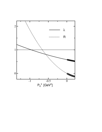
Figure 5.8: The extraporation of the eigenvalue $\lambda$ of the BS equation and R value. The solid line shows the extraporation of the $\lambda$ and the doted line shows the extraporation of the $R$.

Figure 5.9: Extrapolation of the eigenvalue and the $R$ for $\eta^{\prime}$ meson with $G_{D}=75[\mbox{GeV}^{-5}]$.

The obtained mass from the condition $R=1$ is $814[\mbox{MeV}]$ and the mass obtained from the condition $\lambda=1$, where $\lambda$ is the eigenvalue of the BS equation, is $982[\mbox{MeV}]$. This difference of the masses may show the extrapolation uncertainty. Since the dependence of the decay constants $f^{0}_{\eta^{\prime}}$ and $f^{8}_{\eta^{\prime}}$ on the momentum $P_{E}^{2}$ is small, the uncertainty of the decay constants is smaller than that of the masses. Those are shown in Fig. 5.10.

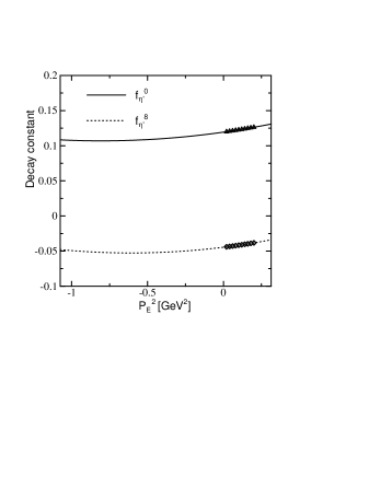
Figure 5.10: Extraporation of the $f^{0}_{\eta^{\prime}}$ and $f^{8}_{\eta^{\prime}}$ with $G_{D}=75[\mbox{GeV}^{-5}]$.

We think that this ambiguity from the extrapolation is unavoidable in the current approach.

5.4 Solution of the BS equation of the Scalar Mesons

In this section, we present the results of the ILA calculation for the scalar mesons. Note that the parameters of the present approach are completely fixed in the study of the pseudoscalar mesons. The results for the $a_{0}$, $\sigma$, $f_{0}$ mesons are summarized in Tables 5.6, 5.7 and 5.8. The dependence of the mass spectrum on the strength, $G_{D}$ of the KMT interaction is shown in Fig. 5.11.

First, the dependencies of the masses of $\sigma$ and $a_{0}$ on $G_{D}$ look qualitatively same as the NJL results shown in Fig.(3.1). In the NJL calculation, the parameters are chosen so as to reproduce the $M_{\pi}$ and $f_{\pi}$ at each $G_{D}$. In contrast, in the ILA approach we change $G_{D}$ independently. However, since $M_{\pi}$ and $f_{\pi}$ depend weakly on $G_{D}$, the results of ILA show similar behavior as those of NJL. We note that the mass of $a_{0}$ grows as $G_{D}$ increases, while the $\sigma$ mass is fairly constant. The behavior of the $f_{0}$ mass differs from the that of NJL model. As noted in Chapter 3, the mass of the $f_{0}$ solution in the NJL model is much higher than the threshold, $2M_{q}$ and the momentum cutoff,$\lambda$. The $f_{0}$ mass in the NJL result is not so reliable.

The $\sigma$ meson mass is predicted as about $670[\mbox{MeV}]$. This rather small $\sigma$ meson mass is interesting. In the case of the NJL model, the $\sigma$ meson mass is determined to be close to twice of the dynamical quark mass. On the other hand, in the ILA approach the value of the mass function at $P_{E}^{2}$, $B_{q}(p_{E}^{2}=0)$ is about $616[\mbox{MeV}]$, which is comparable to the $\sigma$ meson mass. Although there are such differences, the properties of the physical observables agree in both the calculations. This feature is very interesting.

The dependence of the $\sigma$ meson mass on the $G_{D}$ is small. This means that the effects of the $s\bar{s}$ mixing and the KMT interaction are balanced. On the other hand, in the case of $a_{0}$, the flavor content does not change and only the repulsion of the KMT is effective. Thus the $a_{0}$ mass monotonically grows as $G_{D}$ increases. We obtain $M_{a_{0}}=942[\mbox{MeV}]$. This result is comparable to the experimental value $984.8\pm 1.4[\mbox{MeV}]$. We obtain a significant mass splitting between the $\sigma$ and $a_{0}$, about $272[\mbox{MeV}]$. We conclude that the observed $\sigma-a_{0}$ mass splitting can be explained as the $U_{A}(1)$ symmetry breaking effects.

The obtained mass of $f_{0}$ is larger than the mass of $a_{0}$ by about $394\mbox{MeV}$ and they do not become degenerate even if we change the strength of the KMT interaction in our parameter range. Therefore $f_{0}(980)$ may not be identified with the $q\bar{q}$ state. To reproduce $f_{0}(980)$ and the higher $I=0$ scalar meson states, it may be needed to treat mixings of multi-quark states.

$G_{D}[\mbox{GeV}^{-5}]$	$M_{a_{0}}[\mbox{MeV}]$
0	591
25	694
50	808
75	942
100	1128

Table 5.6: Dependences of the solution of the $a_{0}$ BS equation on the strength of the KMT interaction.

$G_{D}[\mbox{GeV}^{-5}]$	$M_{\sigma}[\mbox{MeV}]$	$S^{0}$	$S^{8}$	mixing angle[deg]
0	591	12.9	9.09	-54.7
25	618	13.5	8.40	-58.1
50	645	14.4	7.51	-62.5
75	667	16.0	6.47	-68.0
100	683	18.1	5.25	-73.8

Table 5.7: Dependences of the solution of the $\sigma$meson solution of the coupled channel BS equation on the strength of the KMT interaction.

$G_{D}[\mbox{GeV}^{-5}]$	$M_{f_{0}}[\mbox{MeV}]$	$S^{0}$	$S^{8}$	mixing angle[deg]
0	1205	-21.1	14.9	-54.7
25	1230	-20.8	7.4	-70.5
50	1267	-28.4	3.1	-83.7
75	1336	-35.5	3.8	-83.9
100	1462	-45.9	10.3	-77.3

Table 5.8: Dependences of the solution of the $f_{0}$ meson solution of the coupled channel BS equation on the strength of the KMT interaction.

Figure 5.11: Dependence of the mass spectrum of the $a_{0}$, $\sigma$ and $f_{0}$ mesons on the strength of the KMT interaction.

Next, we consider the mixing angles. We introduce the matrix elements $S^{8}$ and $S^{0}$ which are defined by

$$S^{a}=\int d^{4}x\langle 0|\bar{q}\frac{\lambda^{8}}{2}q(x)|\mbox{scalar meson state}\rangle$$ (5.3)

$$=\mbox{tr}\left[\bar{\chi}^{R}(0;P)\frac{\lambda^{a}}{2}\right]$$ (5.4)

Since these S values extract the particular flavor component of $\phi_{S}$ which is the main component of the BS amplitude at the origin, we employ $S^{8}$ and $S^{0}$ to determine the ratio of the octet and the singlet components. Accordingly we define the mixing angles of the scalar mesons as

$$\tan\theta_{\sigma}=-\frac{S_{0}^{\sigma}}{S_{8}^{\sigma}}$$ (5.5)

$$\tan\theta_{f_{0}}=\frac{S_{8}^{f_{0}}}{S_{0}^{f_{0}}}.$$ (5.6)

The results are summarized in Table 5.6, 5.7 and Fig 5.12.

Figure 5.12: Dependence of the mixing angle of the $\eta$ and $\eta^{\prime}$ meson on the strength of the KMT interaction.

The mixing angle of $\sigma$ approaches $-90^{\circ}$, where $\sigma$ becomes the purely flavor singlet state: $\frac{1}{\sqrt{3}}(u\bar{u}+d\bar{d}+s\bar{s})$. The obtained angle at $G_{D}=75[\mbox{GeV}^{-5}]$ is $-68.0^{\circ}$ and is slightly smaller than the result of the NJL model, $-77.3^{\circ}$. This angle corresponds to about $5\%$ mixing of the strangeness component in $\sigma$.

Finally , the comparison of the scalar and pseudoscalar meson spectra is shown in Fig. $(\ref{FIG:spectrum})$

Figure 5.13: Dependence of the mass spectrum of the $\pi$, $\eta$, $\eta^{\prime}$, $a_{0}$, $\sigma$ and $f_{0}$ mesons on the strength of the KMT interaction.

5.5 Solution of the BS equation of the Strange Mesons

In this section, we calculate the masses of the strange pseudoscalar meson $K$ and the strange scalar meson $K_{0}^{*}$. Here we employ a crude approximation in order to avoid the technical difficulty. As these mesons consists of the a strange quark and a nonstrange quark. Then the BS equation of the ILA approach becomes extremely complicated. Instead of treating the asymmetric BS equation, we solve the symmetric BS equation for the quarks whose mass is $77.25[\mbox{MeV}]$. This mass is the average of $m_{q}$ and $m_{s}$. The results are summarized in Tables 5.9, 5.10 and Fig.(5.14).

$G_{D}[\mbox{GeV}^{-5}]$	$M_{K}[\mbox{MeV}]$
0	547
25	546
50	544
75	538
100	530

Table 5.9: Dependences of the solution of the $K$ meson BS equation on the strength of the KMT interaction.

$G_{D}[\mbox{GeV}^{-5}]$	$M_{K_{0}^{*}}[\mbox{MeV}]$
0	946
25	1040
50	1158
75	1321
100	1542

Table 5.10: Dependences of the solution of the $K_{0}^{*}$ meson BS equation on the strength of the KMT interaction.

Again the $K$ mass depends little on $G_{D}$ as in the case of $\pi$ . On the other hand, the $K_{0}^{*}$ meson mass increases due to the repulsion of the KMT interaction.

Although these results are based on the symmetric BS equations, the obtained $K$ mass, $494\sim 498[\mbox{MeV}]$, reproduces the observed value and $G_{D}$ dependence agrees with that of the NJL.

Figure 5.14: Dependence of the mass spectrum of the scalar and pseudoscalar meson nonet on the strength of the KMT interaction.

One sees that the slopes of the $a_{0}$ mass and $K_{0}^{*}$ mass are nearly equal and therefore it is clear that the $K_{0}^{*}$ mass does not become smaller than the $a_{0}$ mass in this approach. Since the NJL also gives the similar result, we conclude that the reversal of the $\kappa(700-900)$ mass and the $a_{0}(980)$ mass can not be explained by the $U_{A}(1)$ symmetry breaking. Furthermore, our $K_{0}^{*}$ mass is smaller than the next excited state $K_{0}^{*}(1430)$ by about $110\mbox{MeV}$. Consequently, the light $I=1/2$ scalar mesons may not be explained without considering mixings of the multi-quark states.

Chapter 6 Conclusion

We have studied the roles of the $U_{A}(1)$ breaking interaction of QCD in the spectrum of the light scalar nonet mesons using the extended NJL model and the ILA of QCD. We have first analyzed qualitative properties of the $U_{A}(1)$ breaking interaction in the extended NJL model, and next using the ILA approach we have carried out quantitative study. Since these approaches are consistent with chiral symmetry, the scalar and pseudoscalar mesons can be regarded as chiral partners. We choose parameters to reproduce the masses and decay constants of the pseudoscalar nonet mesons and apply those to the scalar nonet mesons.

The extended NJL model is the SU(3) NJL model supplemented with the Kobayashi-Maskawa-’t Hooft (KMT) interaction, which causes the $U_{A}(1)$ breaking. The strength of the KMT interaction is chosen so as to explain the electromagnetic decays of the $\eta$ meson. To study the role of the $U_{A}(1)$ breaking, we study the mass spectrum and the mixing angle of the scalar mesons as functions of the strength of the KMT interaction. As a result, we observe that the $\sigma$ meson mass changes little, which suggests that the increase of the dynamical quark mass and the attractive KMT interaction cancel with each other. On the other hand, the mass of $a_{0}$ increases monotonically due to the repulsive KMT interaction. This $\sigma-a_{0}$ mass splitting amounts to a $150$ MeV and is slightly smaller than the current experimental data. A possible reason that the $a_{0}$ mass is not large enough is the large unphysical $q\mbox{$\bar{q}$}$ decay width which is an artifact of this model. We have also found that the strangeness content in the $\sigma$ meson is about $15\%$.

The ILA of QCD is an approximation that is consistent with chiral symmetry and consists of the rainbow approximation of the Schwinger-Dyson equation and the ladder approximation of the Bethe-Salpeter equation. Using this approach, we analyze the scalar meson spectrum quantitatively. As we do in the extended NJL model, we choose the parameters to reproduce physical observables of the pseudoscalar mesons.

We have obtained that the $\sigma$ meson mass comes around $600\sim 700[\mbox{MeV}]$, which is much lower than the value expected from the effective quark mass. This suggests that the $\sigma$ meson is special as the chiral partner of the pion. We obtain the $\sigma-a_{0}$ mass splitting of about $272[\mbox{MeV}]$ and the strangeness content in the $\sigma$ meson is about $5\%$. It will be interesting to check this $s\bar{s}$ mixing experimentally by using, for instance, the radiative $J/\psi$ decays in near future.

The obtained mass of $f_{0}$ is larger than the mass of $a_{0}$ by about $394\mbox{MeV}$ and they do not become degenerate even if we change the strength of the KMT interaction in our parameter range. Therefore $f_{0}(980)$ may not be identified with the $q\bar{q}$ state. To reproduce $f_{0}(980)$ and the higher $I=0$ scalar meson states, it may be needed to treat mixings of multi-quark states.

The masses of the strange mesons have been calculated in an approximation. We have found that the $K_{0}^{*}$ mass is larger than the $a_{0}$ mass by about $230[\mbox{MeV}]$. The masses of $a_{0}$ and $K_{0}^{*}$ mesons increase by almost the same rate as $G_{D}$ is increased. Therefore it seems that the reversal of the $\kappa(700-900)$ mass and the $a_{0}(980)$ mass can not be explained by the $U_{A}(1)$ symmetry breaking.

Furthermore, our $K_{0}^{*}$ mass is smaller than the next excited state $K_{0}^{*}(1430)$ by about $379\mbox{MeV}$. Consequently, the light $I=1/2$ scalar mesons may not be explained without considering mixings of multi-quark states.

In conclusion, we have shown that the spectra of the pseudoscalar meson nonet and the $\sigma$ and $a_{0}$ masses can be reproduced by the extended Nambu-Jona-Lasinio model and improved ladder approximation of QCD with $U_{A}(1)$ breaking interaction. We have found that the observed spectrum is consistent with the strong $U_{A}(1)$ breaking interaction. Furthermore we have shown that $f_{0}(980)$ and $\kappa(700-900)$ can not be reproduced in our picture. It may be needed to treat mixings of multi-quark states.

For the more detailed analysis, the approach in which the decay width of the mesons may be needed. Such calculations will require two-point correlation functions of mesons in the Minkowski kinematics. This is beyond the scope of the present approach.

As these results have clarified the realization of chiral symmetry in the scalar mesons, it will now be interesting to confirm the results experimentally and also to study behavior of the scalar mesons at finite temperature and/or density, where we expect that chiral symmetry is going toward restoration.

Acknowledgments

I would like to express my deep gratitude for my supervisor prof. M. Oka who has shared his deep insight in physics with me. I have benefited very much from our many discussions and his lectures. He has also patiently answered my questions.

I also thank Dr. M. Takizawa for useful discussions and comments about the NJL model, K. Naito for the discussions about the ILA approach and M. Ishida for useful comment about the scalar nonet mesons.

Appendix A BS Equation

Here we show the explicit form of the BS equation. At first, we define the regularized amputated BS amplitude $\hat{\chi}^{R}(q;P)$ by

$$\hat{\chi}^{R}(q;P)={S_{F}^{R}}^{-1}(q+\frac{P}{2})\chi^{R}(q;P){S_{F}^{R}}^{-1}(q-\frac{P}{2})$$ (A.1)

By introducing the $\hat{\phi}_{A}$ which denotes the set of the amplitudes of the $\hat{\chi}^{R}(q;P)$ , the BS equation can be written as

$$\hat{\phi}(q;P)=\int_{k}K_{AB}(q,k;P)\phi_{B}(k;P).$$ (A.2)

We solve the BS equation by dividing to these two part.

The explicit form of Eq. (A.1) is given by

$$\phi_{S}=\frac{1}{\Delta}\left[\begin{array}[]{l}\quad\left\{-{q_{E}}^{2}+\frac{{P_{E}}^{2}}{4}-B_{+}B_{-}\right\}\hat{\phi}_{S}\\ +\left\{-{q_{E}}^{2}(B_{+}-B_{-})+\frac{{P_{E}}{q_{E}}}{2}(B_{+}+B_{-})\right\}\hat{\phi}_{P}\\ +\left\{\frac{{P_{E}}^{2}}{2}(B_{+}+B_{-})-{P_{E}}{q_{E}}(B_{+}-B_{-})\right\}\hat{\phi}_{Q}\\ +\left\{{q_{E}}^{2}{P_{E}}^{2}-({P_{E}}{q_{E}})^{2}\right\}\hat{\phi}_{T}\\ \end{array}\right]$$ (A.7)

$$\phi_{P}=\frac{1}{\Delta}\left[\begin{array}[]{l}\quad\left\{B_{+}-B_{-}\right\}\hat{\phi}_{S}\\ +\left\{-{q_{E}}^{2}-\frac{{P_{E}}^{2}}{4}-B_{+}B_{-}\right\}\hat{\phi}_{P}\\ +\left\{-2{P_{E}}{q_{E}}\right\}\hat{\phi}_{Q}\\ +\left\{({P_{E}}{q_{E}})(B_{+}+B_{-})-\frac{{P_{E}}^{2}}{2}(B_{+}-B_{-})\right\}\hat{\phi}_{T}\\ \end{array}\right]$$ (A.12)

$$\phi_{Q}=\frac{1}{\Delta}\left[\begin{array}[]{l}\quad\left\{-\frac{1}{2}(B_{+}+B_{-})\right\}\hat{\phi}_{S}\\ +\left\{\frac{1}{2}{P_{E}}{q_{E}}\right\}\hat{\phi}_{P}\\ +\left\{\left({q_{E}}^{2}+\frac{{P_{E}}^{2}}{4}\right)-B_{+}B_{-}\right\}\hat{\phi}_{Q}\\ +\left\{-{q_{E}}^{2}(B_{+}+B_{-})+\frac{{P_{E}}{q_{E}}}{2}(B_{+}-B_{-})\right\}\hat{\phi}_{T}\\ \end{array}\right]$$ (A.17)

$$\phi_{T}=\frac{1}{\Delta}\left[\begin{array}[]{l}\quad\hat{\phi}_{S}\\ +\left\{\frac{1}{2}(B_{+}-B_{-})\right\}\hat{\phi}_{P}\\ +\left\{B_{+}+B_{-}\right\}\hat{\phi}_{Q}\\ +\left\{{q_{E}}^{2}-\frac{{P_{E}}^{2}}{4}-B_{+}B_{-}\right\}\hat{\phi}_{T}\\ \end{array}\right]$$ (A.22)

where

$$q_{E+}=q+\frac{P}{2}\qquad q_{E-}=q-\frac{P}{2}$$ (A.23)

$$B_{+}=B(q_{E+}^{2})\qquad B_{-}=-B(q_{E-}^{2})$$ (A.24)

$$\Delta=({q_{E}}_{+}^{2}+B_{+}^{2})({q_{E}}_{-}^{2}+B_{-}^{2}).$$ (A.25)

The explicit form of the ${\cal L}_{\rm GE}$ part of the interaction kernel $K$ in the Eq. (A.1) is given by

$$K^{(E)}_{SS}=C_{F}\frac{\bar{g}^{2}}{f^{2}}\frac{\lambda^{\alpha}}{2}\left[\frac{-3}{(q_{E}-k_{E})^{2}}\right]$$ (A.26)

$$K^{(E)}_{PP}=C_{F}\frac{\bar{g}^{2}}{f^{2}}\frac{\lambda^{\alpha}}{2}\left[\frac{1}{(q_{E}-k_{E})^{2}}\frac{k_{q}}{A}+\frac{2}{(q_{E}-k_{E})^{4}}(q_{E}-k_{E})\cdot k_{E}\left(1-\frac{k_{q}}{A}\right)\right]$$ (A.27)

$$K^{(E)}_{QP}=C_{F}\frac{\bar{g}^{2}}{f^{2}}\frac{\lambda^{\alpha}}{2}\left[\frac{1}{(q_{E}-k_{E})^{2}}\frac{k_{P}}{A}-\frac{2}{(q_{E}-k_{E})^{4}}(q_{E}-k_{E})\cdot k_{E}\left(\frac{k_{P}}{A}\right)\right]$$ (A.28)

$$K^{(E)}_{QQ}=C_{F}\frac{\bar{g}^{2}}{f^{2}}\frac{\lambda^{\alpha}}{2}\left[\frac{1}{(q_{E}-k_{E})^{2}}-\frac{2}{(q_{E}-k_{E})^{4}}(q_{E}-k_{E})\cdot P_{E}\left(\frac{k_{P}}{A}\right)\right]$$ (A.29)

$$K^{(E)}_{PQ}=C_{F}\frac{\bar{g}^{2}}{f^{2}}\frac{\lambda^{\alpha}}{2}\left[\frac{2}{(q_{E}-k_{E})^{4}}(q_{E}-k_{E})\cdot P_{E}\left(1-\frac{k_{q}}{A}\right)\right]$$ (A.30)

$$K^{(E)}_{TT}=C_{F}\frac{\bar{g}^{2}}{f^{2}}\frac{\lambda^{\alpha}}{2}\left[\frac{(k_{E}^{2}-q_{E}^{2})\left(-\frac{k_{q}}{A}\right)+2(q_{E}-k_{E})\cdot P_{E}\frac{k_{P}}{A}-2(q_{E}-k_{E})\cdot k_{E}}{(q_{E}-k_{E})^{4}}\right]$$ (A.31)

where

$$A=q_{E}^{2}P_{E}^{2}-(P_{E}\cdot q_{E})^{2}$$ (A.32)

$$k_{q}=P_{E}^{2}(q_{E}\cdot k_{E})-(P_{E}\cdot q_{E})(P_{E}\cdot k_{E})$$ (A.33)

$$k_{P}=q_{E}^{2}(P_{E}\cdot k_{E})-(q_{E}\cdot P_{E})(q_{E}\cdot k_{E}).$$ (A.34)

The ${\cal L}_{\rm KMT}$ part is given by

$$K^{(E)}_{SS}=-24G_{D}\epsilon^{ghf^{\prime}}\epsilon^{fh^{\prime}g^{\prime}}\mbox{tr}[{S_{F}}(p)]_{h^{\prime}h}\left[\frac{\lambda^{q}}{2}\phi_{S}^{q}(q;P)+\frac{\lambda^{s}}{2}\phi_{S}^{s}(q;P)\right]_{g^{\prime}h}.$$ (A.35)

Appendix B Normalization Condition of the BS Amplitude

Here we show the normalization condition of the BS amplitude explicitly.

To reduce the expressions we use abbreviation

$$B_{+}=B\left(\left(q_{E}+P_{E}/2\right)^{2}\right)$$ (B.1)

$$B_{-}=B\left(\left(q_{E}-P_{E}/2\right)^{2}\right)$$ (B.2)

$$\rho_{+E}=(q_{E}+P_{E}/2)^{2}$$ (B.3)

$$\rho_{-E}=(q_{E}-P_{E}/2)^{2}$$ (B.4)

$$\Phi=\chi^{R}(q;P)$$ (B.5)

$$\tilde{\Phi}=\bar{\chi}^{R}(q;P).$$ (B.6)

The normalization condition of the BS amplitude is given by

$$\frac{N_{C}}{2}\int_{q_{E}} \frac{1}{f({q_{E}}_{+}^{2})f({q_{E}}_{-}^{2})}$$

$$\times \left\{\frac{1}{2}\mbox{tr}[\tilde{\Phi}P\!\!\!\!/_{E}\Phi q\!\!\!/_{E}]-\frac{1}{4}\mbox{tr}[\tilde{\Phi}P\!\!\!\!/_{E}\Phi P\!\!\!\!/_{E}]-\frac{1}{2}B_{-}\mbox{tr}[\tilde{\Phi}P\!\!\!\!/_{E}\Phi]-\left(P_{E}q_{E}+\frac{P_{E}^{2}}{2}\right)B^{\prime}_{+}\mbox{tr}[\tilde{\Phi}\Phi q\!\!\!/_{E}]\right.$$ (B.7)

$$\qquad+\frac{1}{2}\left(P_{E}q_{E}+\frac{P_{E}^{2}}{2}\right)B^{\prime}_{+}\mbox{tr}[\tilde{\Phi}\Phi P\!\!\!\!/_{E}]+\left(P_{E}q_{E}+\frac{P_{E}^{2}}{2}\right)B^{\prime}_{+}B_{-}\mbox{tr}[\tilde{\Phi}\Phi]$$

$$\quad-\frac{1}{2}\mbox{tr}[\tilde{\Phi}q\!\!\!/_{E}\Phi P\!\!\!\!/_{E}]-\frac{1}{4}\mbox{tr}[\tilde{\Phi}P\!\!\!\!/_{E}\Phi P\!\!\!\!/_{E}]+\frac{1}{2}B_{+}\mbox{tr}[\tilde{\Phi}\Phi P\!\!\!\!/_{E}]-\left(-P_{E}q_{E}+\frac{P_{E}^{2}}{2}\right)B^{\prime}_{-}\mbox{tr}[\tilde{\Phi}q\!\!\!/_{E}\Phi]$$

$$\qquad\left.-\frac{1}{2}\left(-P_{E}q_{E}+\frac{P_{E}^{2}}{2}\right)B^{\prime}_{-}\mbox{tr}[\tilde{\Phi}P\!\!\!\!/_{E}\Phi]+\left(-P_{E}q_{E}+\frac{P_{E}^{2}}{2}\right)B_{+}B^{\prime}_{-}\mbox{tr}[\tilde{\Phi}\Phi]\right\}$$

$$=2P_{E}^{2}$$

where

$$\mbox{tr}[\tilde{\Phi}P\!\!\!\!/_{E}\Phi q\!\!\!/_{E}]= 4\left(-\phi_{S}(-q;P)\phi_{S}(q;P)P_{E}q_{E}-\phi_{S}(-q;P)\phi_{T}(q;P)((P_{E}q_{E})^{2}-P_{E}^{2}q_{E}^{2})\right.$$ (B.8)

$$\quad-\phi_{T}(-q;P)\phi_{S}(q;P)((P_{E}q_{E})^{2}-P_{E}^{2}q_{E}^{2})+\phi_{P}(-q;P)\phi_{P}(q;P)q_{E}^{2}P_{E}q_{E}$$

$$\quad+\phi_{P}(-q;P)\phi_{Q}(q;P)(P_{E}q_{E})^{2}-\phi_{Q}(-q;P)\phi_{P}(q;P)q_{E}^{2}P_{E}^{2}$$

$$\quad\left.-\phi_{Q}(-q;P)\phi_{Q}(q;P)P_{E}^{2}P_{E}q_{E}\right)$$

$$\mbox{tr}[\tilde{\Phi}q\!\!\!/_{E}\Phi P\!\!\!\!/_{E}]= 4\left(-\phi_{S}(-q;P)\phi_{S}(q;P)P_{E}q_{E}+\phi_{S}(-q;P)\phi_{T}(q;P)((P_{E}q_{E})^{2}-P_{E}^{2}q_{E}^{2})\right.$$ (B.9)

$$\quad+\phi_{T}(-q;P)\phi_{S}(q;P)((P_{E}q_{E})^{2}-P_{E}^{2}q_{E}^{2})+\phi_{P}(-q;P)\phi_{P}(q;P)q_{E}^{2}P_{E}q_{E}$$

$$\quad+\phi_{P}(-q;P)\phi_{Q}(q;P)q_{E}^{2}P_{E}^{2}-\phi_{Q}(-q;P)\phi_{P}(q;P)(P_{E}q_{E})^{2}$$

$$\quad\left.-\phi_{Q}(-q;P)\phi_{Q}(q;P)P_{E}^{2}P_{E}q_{E}\right)$$

$$\mbox{tr}[\tilde{\Phi}P\!\!\!\!/_{E}\Phi P\!\!\!\!/_{E}]= 4\left(-\phi_{S}(-q;P)\phi_{S}(q;P)P_{E}^{2}-\phi_{T}(-q;P)\phi_{T}(q;P)P_{E}^{2}\{(P_{E}q_{E})^{2}-P_{E}^{2}q_{E}^{2}\}\right.$$ (B.10)

$$\quad+\phi_{P}(-q;P)\phi_{P}(q;P)(P_{E}q_{E})^{2}+\phi_{P}(-q;P)\phi_{Q}(q;P)P_{E}^{2}P_{E}q_{E}$$

$$\quad\left.-\phi_{Q}(-q;P)\phi_{P}(q;P)P_{E}^{2}P_{E}q_{E}-\phi_{Q}(-q;P)\phi_{Q}(q;P)P_{E}^{4}\right)$$

$$\mbox{tr}[\tilde{\Phi}P\!\!\!\!/_{E}\Phi]= -4\left(-\phi_{S}(-q;P)\phi_{P}(q;P)P_{E}q_{E}-\phi_{P}(-q;P)\phi_{S}(q;P)P_{E}q_{E}\right.$$ (B.11)

$$\quad-\phi_{S}(-q;P)\phi_{Q}(q;P)P_{E}^{2}+\phi_{Q}(-q;P)\phi_{S}(q;P)P_{E}^{2}$$

$$\quad-\phi_{T}(-q;P)\phi_{P}(q;P)\{(P_{E}q_{E})^{2}-P_{E}^{2}q_{E}^{2}\}$$

$$\quad\left.-\phi_{P}(-q;P)\phi_{T}(q;P)\{(P_{E}q_{E})^{2}-P_{E}^{2}q_{E}^{2}\}\right)$$

$$\mbox{tr}[\tilde{\Phi}\Phi P\!\!\!\!/_{E}]= -4\left(-\phi_{S}(-q;P)\phi_{P}(q;P)P_{E}q_{E}-\phi_{P}(-q;P)\phi_{S}(q;P)P_{E}q_{E}\right.$$ (B.12)

$$\quad-\phi_{S}(-q;P)\phi_{Q}(q;P)P_{E}^{2}+\phi_{Q}(-q;P)\phi_{S}(q;P)P_{E}^{2}$$

$$\quad+\phi_{T}(-q;P)\phi_{P}(q;P)\{(P_{E}q_{E})^{2}-P_{E}^{2}q_{E}^{2}\}$$

$$\quad\left.+\phi_{P}(-q;P)\phi_{T}(q;P)\{(P_{E}q_{E})^{2}-P_{E}^{2}q_{E}^{2}\}\right)$$

$$\mbox{tr}[\tilde{\Phi}q\!\!\!/_{E}\Phi]= -4\left(-\phi_{S}(-q;P)\phi_{P}(q;P)q_{E}^{2}-\phi_{P}(-q;P)\phi_{S}(q;P)q_{E}^{2}\right.$$ (B.13)

$$\quad-\phi_{S}(-q;P)\phi_{Q}(q;P)P_{E}q_{E}+\phi_{Q}(-q;P)\phi_{S}(q;P)P_{E}q_{E}$$

$$\quad+\phi_{T}(-q;P)\phi_{Q}(q;P)\{(P_{E}q_{E})^{2}-P_{E}^{2}q_{E}^{2}\}$$

$$\quad\left.-\phi_{Q}(-q;P)\phi_{T}(q;P)\{(P_{E}q_{E})^{2}-P_{E}^{2}q_{E}^{2}\}\right)$$

$$\mbox{tr}[\tilde{\Phi}\Phi q\!\!\!/_{E}]= -4\left(-\phi_{S}(-q;P)\phi_{P}(q;P)q_{E}^{2}-\phi_{P}(-q;P)\phi_{S}(q;P)q_{E}^{2}\right.$$ (B.14)

$$\quad-\phi_{S}(-q;P)\phi_{Q}(q;P)P_{E}q_{E}+\phi_{Q}(-q;P)\phi_{S}(q;P)P_{E}q_{E}$$

$$\quad-\phi_{T}(-q;P)\phi_{Q}(q;P)\{(P_{E}q_{E})^{2}-P_{E}^{2}q_{E}^{2}\}$$

$$\quad\left.+\phi_{Q}(-q;P)\phi_{T}(q;P)\{(P_{E}q_{E})^{2}-P_{E}^{2}q_{E}^{2}\}\right)$$

$$\mbox{tr}[\tilde{\Phi}\Phi]= 4\left(\phi_{S}(-q;P)\phi_{S}(q;P)-\phi_{P}(-q;P)\phi_{P}(q;P)q_{E}^{2}-\phi_{P}(-q;P)\phi_{Q}(q;P)P_{E}q_{E}\right.$$

$$\quad+\phi_{Q}(-q;P)\phi_{P}(q;P)P_{E}q_{E}+\phi_{Q}(-q;P)\phi_{Q}(q;P)P_{E}^{2}$$

$$\quad\left.-\phi_{T}(-q;P)\phi_{T}(q;P)\{(P_{E}q_{E})^{2}-P_{E}^{2}q_{E}^{2}\}\right).$$

Bibliography

- [1] S. Weinberg, Phys. Rev. D 11 (1975), 3583.
- [2] G. ’t Hooft, Phys. Rev. Lett. 37 (1976), 8; Phys. Rev. D 14 (1976), 3432.
- [3] For a review, T. Schäfer and E. V. Shuryak, Rev. Mod. Phys. 70 (1998), 323.
- [4] M. Takizawa, Y. Nemoto and M. Oka, Phys. Rev. D 55 (1997), 4083.
- [5] See for recent developments, Proceedings of the workshop “Possible existence of the -meson and its implications to hadron physics”, June 2000, Yukawa Institute for Theoretical Physics, Kyoto, Japan, KEK-Proceedings 2000-4, Dec. 2000 and Soryushiron Kenkyu (Kyoto) 102 (2001).
- [6] Particle Data Group, K. Hagiwara et al., Phys. Rev. D 66 (2002), 010001-450 and references therein.
- [7] Wu Ning (BES collaboration), hep-ex/0104050.
- [8] T. Hatsuda and T. Kunihiro, Phys. Rev. Lett. 55 (1985), 158; T. Hatsuda, T. Kunihiro and H. Shimizu, Phys. Rev. Lett. 82 (1999), 2840.
- [9] D. Black, A. H. Fariborz, S. Moussa, S. Nasri and J. Schechter, Phys. Rev. D 64 (2001), 014031, and references therein.
- [10] J. A. Oller and E. Oset, Phys. Rev. Lett. 80 (1998), 3452, and references therein.
- [11] Y. Nambu and G. Jona-Lasinio, Phys. Rev, 122 (1961) 345; 124 (1961) 246.
- [12] M. Kobayashi and T. Maskawa, Prog. Theor. Phys. 44 (1970), 1422; M. Kobayashi, H. Kondo and T. Maskawa, Prog. Theor. Phys. 45 (1971), 1955.
- [13] K. Higashijima, Phys. Rev. D29 (1984) 1228; V.A. Miransky, Sov. J. Nucl. Phys. 38 (1984) 280.
- [14] K. Aoki, M. Bando, T. Kugo, M.G. Mitchard and H. Nakatani, Prog. Theor. Phys 84 (1990) 683; K-I. Aoki and M. Mitchard, Phys. Lett. B266 (1991) 467.
- [15] K-I. Aoki, K. Takagi, H. Terao, M. Tomoyose, Prog. Theor. Phys. 103 (2000) 815;
- [16] K. Naito, K. Yoshida, Y. Nemoto, M. Oka and M. Takizawa, Phys.Rev. C59 (1999) 1095-1106; K. Naito and M. Oka, Phys.Rev. C59 (1999) 542-545.
- [17] K. Naito, K. Yoshida, Y. Nemoto, M. Oka and M. Takizawa, Phys.Rev. C59 (1999) 1722-1734.
- [18] K. Naito, Y. Nemoto, M. Takizawa, K. Yoshida and M. Oka, Phys. Rev. C 61 (2000), 065201.
- [19] T. Hatsuda and T. Kunihiro, Phys. Rep. 247 (1994), 221.
- [20] C. M. Shakin, Phys. Rev. D 65 (2002), 114011.
- [21] V.Dmitrasinovic, Phys. Rev. C 53 (1996), 1383.
- [22] L. H. Chan and R. W. Haymaker, Phys. Rev. D 10 (1974), 4143; M. Ishida, Prog. Theor. Phys. 101 (1999), 661-669.
- [23] A. A. Belavin, A. M. Polyakov, A. A. Schwartz, and Y. S. Tyupkin, Phys. Lett. B59 (1975), 85;
- [24] E. V. Shuryak, Nucl. Phys. B 203 (1982), 93; B 203 (1982), 116.
- [25] M. Takizawa, K. Tsushima, Y. Kohyama and K. Kubodera, Nucl. Phys. A 507 (1990), 611.
- [26] M. Takizawa, K. Kubodera and F. Myhrer, Phys. Lett. B 261 (1991), 221.
- [27] T. Kunihiro and T. Hatsuda, Phys. Lett. B206 (1988) 385; T. Hatsuda and T. Kunihiro, Z. Phys. C51 (1991) 49; V. Bernard, R.L. Jaffe and U.-G. Meissner, Nucl. Phys.B308 (1988) 753; M. Takizawa, K. Tsushima, Y. Kohyama and K. Kubodera, Prog. Theor. Phys. 82 (1989)481; Nucl. Phys. A507(1990) 611; H. Reinhardt and R. Alkofer, Phys. Lett. B207 (1988) 482; R. Alkofer and H. Reinhardt, Z. Phys C45 (1989) 275; S. Klimt, M. Lutz, U. Vogl and W. Weise, Nucl. Phys. A516 (1990) 429; U.Vogl, M. Lutz, S. Klimt and W. Weise, Prog. Part. Nucl. Phys. 27 (1991) 195.
- [28] Y. Nemoto, M. Oka and M. Takizawa, Phys. Rev. D 54, 6477 (1996); M. Takizawa and M. Oka, Phys. Lett B 359, 210 (1995); 364, 249(E) (1995).
- [29] J.M. Cornwall, R. Jackiw, E. Tomboulis, Phys. Rev. D10 (1974) 2428.