A detailed QCD analysis of twist-3 effects in DVCS observables

Abstract

In this paper I present a detailed QCD analysis of twist-3 effects in the Wandzura-Wilczek (WW) approximation in deeply virtual Compton scattering (DVCS) observables for various kinematical settings, representing the HERA , HERMES, CLAS and the planned EIC (electron-ion-collider) experiments. I find that the twist-3 effects in the WW approximation are almost always negligible at collider energies but can be large for low $Q^{2}$ and smaller $x_{bj}$ in observables for the lower energy, fixed target experiments directly sensitive to the real part of DVCS amplitudes like the charge asymmetry (CA). Conclusions are then drawn about the reliability of extracting twist-2 generalized parton distributions (GPDs) from experimental data and a first, phenomenological, parameterization of the LO and NLO twist-2 GPD $H$, describing all the currently available DVCS data within the experimental errors is given.

PACS numbers: 11.10.Hi, 11.30.Ly, 12.38.Bx

I Introduction

Hard, exclusive processes and amongst them deeply virtual Compton scattering (DVCS) in particular mrgdh ; ji ; rad1 ; die ; vgg ; jcaf ; ffgs ; ffs ; gb1 ; gb2 ; bemuothers , have emerged in recent years as prime candidates to gain a three dimensional foot1 image of parton correlations inside a nucleon afgpd3d ; burk12 ; diehl3d ; bemunew ; ji3dnew . This information is gained by mapping out the key component containing this three dimensional information, namely generalized parton distributions (GPDs).

GPDs have been studied extensively in recent years mrgdh ; ji ; rad1 ; die ; vgg ; jcaf ; ffgs ; ffs ; gb1 ; gb2 ; bemuothers ; shupoly since these distributions are not only the basic, non-perturbative ingredient in hard, exclusive processes such as DVCS or exclusive vector meson production, they are generalizations of the well known parton distribution functions (PDFs) from inclusive reactions. GPDs incorporate both a partonic and distributional amplitude behavior and hence contain more information about the hadronic degrees of freedom than PDFs. In fact, GPDs are true two-parton correlation functions, allowing access to highly non-trivial parton correlations inside hadrons foot .

In order to perform a mapping of GPDs in their variables, experimental data from a wide variety of hard, exclusive processes is needed. Furthermore, in order to be able to properly interpret the data, the processes should be well understood theoretically. Therefore, one should start out exploring the theoretically “simplest” process i.e. the one with the least theoretical uncertainty. In the class of hard, exclusive processes this is DVCS ($e(k)+p(P)\to e(k^{\prime})+p(P^{\prime})+\gamma(q^{\prime})$). The reason for this is the simple structure of its factorization theorem ji ; rad1 ; jcaf . The scattering amplitude is simply given by the convolution of a hard scattering coefficient computable to all orders in perturbation theory with ${\it one}$ type of GPD carrying the non-perturbative information. Factorization theorems for other hard exclusive processes are usually ${\it double}$ convolutions containing more than one non-perturbative function.

As with all factorization theorems, the DVCS scattering amplitude is given in this simple convolution form up to terms which are suppressed in the large scale of the process. In this case the large scale is the transfered momentum i.e. the virtual photon momentum, $Q$, and the suppressed terms are of the order $O((m_{N}/Q)^{n}),O((\sqrt{-t}/Q)^{n},O((\lambda_{QCD}/Q)^{n})$ with $m_{N}$ the proton mass and $t=(P-P^{\prime})^{2}$ the momentum transfer onto the outgoing proton. This means, however, that for smaller values of $Q$ these uncontrolled terms, called higher twist corrections, could in principle be sizeable and the convolution or lowest twist term need not be the leading one. Since we are interested in the extraction of the non-perturbative information of the lowest twist GPD, in this case twist-2, we need to understand something about these higher twist corrections.

It was shown by several groups bemutw3 ; radweitw3 ; antertw3 ; kivpoly that the first suppressed term (twist-3) in the DVCS scattering amplitude can, in leading order of the strong coupling constant (LO) and in the Wandzura-Wilczek (WW) approximation, be simply expressed through a sum of terms which can be written as a convolution of a LO twist-3 hard scattering coefficient with a twist-2 GPD. Unfortunately, it could not be shown that twist-3 in the WW approximation does factorize to all orders in perturbation theory (it seems to hold in NLO though kivmach ). However, we do have at least some control over the leading of the higher twist terms and can therefore use parameterizations of twist-2 GPDs also for twist-3.

Equipped with this knowledge one might think that this information is enough to obtain an unambiguous interpretation of DVCS data in terms of GPDs, but life is unfortunately even more complicated. Besides the dynamical twist contributions to the amplitude, there are kinematical power corrections in the DVCS cross section i.e. contributions where a dynamical twist-2 amplitude is multiplied by a term $\propto(\sqrt{-t}/Q,m_{N}/Q)$ which makes them of the same power in $1/Q$ as twist-3. These terms are of particular importance in the interference term between DVCS and the QED Bethe-Heitler (BH) process which both contribute to the total DVCS cross section. Since the kinematical power corrections are nothing but dynamical twist-2 with a kinematical dressing they can be handled by the same GPD parameterization as dynamical twist-2. Thus we have the leading corrections to the DVCS process under control, at least in LO, and can now investigate several things: a) How big are physical observables at various values of $x_{bj},Q^{2}$ and $t$ for a certain center-of-mass energy $s$, especially those terms isolating various parts in the interference term directly proportional to real or imaginary parts of DVCS amplitudes? b) How big are the next-to-leading order (NLO) corrections in the strong coupling constant to these observables? c) How big are the corrections to these observables due to twist-3 effects? d) How reliably can the twist-2 GPDs be extracted from DVCS data?

In this paper I will concentrate on c) and d). a) and b) have been extensively discussed using various GPD models in afmmlong ; afmmshort ; bemu3 . c) and d) have, in various forms, been discussed in bemu4 ; vanderhagen1 . This was done, however, without taking evolution effects into account. We know that evolution effects are sizeable and can change the shape of the GPD in the ERBL region substantially afmmgpd , thereby strongly affecting the real part of the amplitude afmmamp and the observables associated with the real part. In afmmlong ; afmmshort it was demonstrated that the type of GPD models most commonly used cannot be brought into agreement with the available data once evolution effects were taken into account. Subsequently, in afmmms , a model was proposed which was able to describe all currently available DVCS data within a full NLO QCD analysis.

I will extend the analysis of afmmms , by not only using the input model of afmmms for the twist-2 GPDs but also as an input for the twist-3 sector in the WW approximation. Sec. II contains the DVCS kinematics, structure of the cross section, equations for the twist-3 contributions and the definition of the relevant observables. In Sec. III, I will recapitulate the model I use for the four relevant twist-2 GPDs $H,\tilde{H},E,\tilde{E}$ and their twist-3 counter parts. Sec. IV contains the twist-2 vs. twist-3 results for DVCS observables in various kinematical settings. In Sec. V, I will present for the first time a phenomenological parameterization of the twist-2 GPD $H$ which can describe all currently available DVCS data within the experimental errors in both LO and NLO QCD. I will then summarize in Sec. VI.

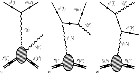
Figure 1: a) DVCS graph, b) BH with photon from final state lepton and c) with photon from initial state lepton.

II DVCS: Kinematics, cross section and definitions

The lepton level process, $e^{\pm}(k,\kappa)~{}N(P,S)\to e^{\pm}(k^{\prime},\kappa^{\prime})~{}N(P^{\prime},S^{\prime})~{}\gamma(q^{\prime},\epsilon^{\prime})$, receives contributions from each of the graphs shown in Fig. 1. This means that the cross section will contain a pure DVCS-, a pure BH- and an interference term.

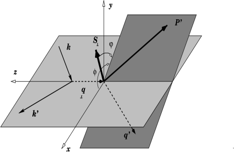
Figure 2: The kinematics of the leptoproduction in the target rest frame.

I choose to work in the target rest frame given in bemu4 (see Fig. 2), where the positive $z$-direction is chosen along the three-momentum of the incoming virtual photon. The incoming and outgoing lepton three-momenta form the lepton scattering plane, while the final state proton and outgoing real photon define the hadron scattering plane. In this reference frame the azimuthal angle of the scattered lepton is $\phi_{l}=0$, while the azimuthal angle between the lepton plane and the final state proton momentum is $\phi_{N}=\phi$. When the hadron is transversely polarized (within this frame of reference) $S_{\perp}=(0,\cos{\mit\Phi},\sin{\mit\Phi},0)$ and the angle between the polarization vector and the scattered hadron is given by $\varphi={\mit\Phi}-\phi_{N}$. The four vectors are $k=(E,E\sin\theta_{l},0,E\cos\theta_{l})$, $q=(q^{0},0,0,-|q^{3}|)$. Other vectors are $P=(M,0,0,0)$ and $P^{\prime}=(E^{\prime},|\mbox{\boldmath$P^{\prime}$}|\cos\phi\sin\theta_{N},|\mbox{\boldmath$P^{\prime}$}|\sin\phi\sin\theta_{N},|\mbox{\boldmath$P^{\prime}$}|\cos\theta_{N})$. The longitudinal part of the polarization vector is $S_{\rm LP}=(0,0,0,\Lambda)$. The relevant Lorentz-invariant variables for DVCS are then:

$$\xi=\frac{Q^{2}}{2{\bar{P}}\cdot{\bar{q}}}\,,{\bar{\cal Q}}^{2}=-{\bar{q}}^{2},t=\Delta^{2}=(P-P^{\prime})^{2}\,,y=\frac{P\cdot q}{P\cdot k}\,,$$

where ${\bar{P}}=(P+P^{\prime})/2$, ${\bar{q}}=(q+q^{\prime})/2$ and which are related to the experimentally accessible variables, $\zeta\equiv x_{bj}=-q^{2}/2P\cdot q$ and $Q^{2}=-q^{2}$, used throughout this paper, via

$${\bar{\cal Q}}^{2}=\frac{1}{2}Q^{2}\left(1+\frac{t}{Q^{2}}\right)\approx\frac{1}{2}Q^{2}$$

$$\xi=\frac{\zeta\left(1+\frac{t}{2Q^{2}}\right)}{2-\zeta\left(1-\frac{t}{Q^{2}}\right)}\approx\frac{\zeta}{2-\zeta}\,.$$ (1)

Note that $t$ has a minimal value given by

$$-t_{\rm min}^{2}=Q^{2}\frac{2(1-x_{bj})\left(1-\sqrt{1+\epsilon^{2}}\right)+\epsilon^{2}}{4x_{bj}(1-x_{bj})+\epsilon^{2}}\,.$$ (2)

where $\epsilon^{2}=4M^{2}x_{bj}^{2}/Q^{2}$. Thus the theoretical limit $t\to 0$ in an exclusive quantity is not attainable in any experimental set-up and one will have to rely on extrapolations.

The corresponding differential cross section is given by bemu4 :

$$d\sigma= \frac{(2\pi)^{4}}{4k\cdot P}|{\cal T}^{\pm}|^{2}\delta^{(4)}(k+P-k^{\prime}-P^{\prime}-q^{\prime})\times$$

$$\frac{d^{3}{\bf k^{\prime}}}{2k^{\prime}_{0}(2\pi)^{3}}\frac{d^{3}{\bf P^{\prime}}}{2P^{\prime}_{0}(2\pi)^{3}}\frac{d^{3}{\bf q^{\prime}}}{2q^{\prime}_{0}(2\pi)^{3}}\,,$$ (3)

and after integrating out some of the phase space we are left with a five-fold differential cross section:

$$\frac{d\sigma}{dx_{bj}dyd|t|d\phi d\varphi}=\frac{\alpha^{3}x_{bj}y}{16\,\pi^{2}\,Q^{2}\sqrt{1+\epsilon^{2}}}\left|\frac{\cal T}{e^{3}}\right|^{2}\,.$$ (4)

The square of the amplitude receives contributions from pure DVCS (Fig. 1a), from pure BH (Figs. 1b, 1c) and from their interference (with a sign governed by the lepton charge),

$$|{\cal T}|^{2}=|{\cal T}_{DVCS}|^{2}+{\cal I}+|{\cal T}_{BH}|^{2}$$ (5)

where the individual terms are given by

$$|{\cal T}_{\rm BH}|^{2}=\frac{e^{6}}{x_{bj}^{2}y^{2}(1+\epsilon^{2})^{2}t\,{\cal P}_{1}(\phi){\cal P}_{2}(\phi)}\times$$

$$\left[c^{\rm BH}_{0}+\sum_{n=1}^{2}c^{\rm BH}_{n}\,\cos(n\phi)+s^{\rm BH}_{1}\,\sin(\phi)\right]$$ (6)

$$|{\cal T}_{\rm DVCS}|^{2}=\frac{e^{6}}{y^{2}{\cal Q}^{2}}\times$$

$$\Big{[}c^{\rm DVCS}_{0}+\sum_{n=1}^{2}\left[c^{\rm DVCS}_{n}\cos(n\phi)+s^{\rm DVCS}_{n}\sin(n\phi)\right]\Big{]}$$ (7)

$${\cal I}=\frac{\pm e^{6}}{x_{bj}y^{3}t{\cal P}_{1}(\phi){\cal P}_{2}(\phi)}$$

$$\Big{[}c_{0}^{\cal I}+\sum_{n=1}^{3}\left[c_{n}^{\cal I}\cos(n\phi)+s_{n}^{\cal I}\sin(n\phi)\right]\Big{]}$$ (8)

where the $+/-$ sign in the interference stands for a negatively/positively charged lepton.

The $c_{n}$’s and $s_{n}$’s are the Fourier coefficients of the $\cos(n\phi)$ and $\sin(n\phi)$ terms. These coefficients are given as combinations of the real and imaginary part of the unpolarized and the polarized proton spin-non-flip and spin-flip DVCS amplitudes ${\cal H},{\cal\tilde{H}},{\cal E},{\cal\tilde{E}}$ (for the $c^{\cal I}$’s or $s^{\cal I}$’s) or the squares of the afore mentioned DVCS amplitudes (for the $c^{\rm DVCS}$’s or $s^{\rm DVCS}$’s). The exact from is given in bemu4 and does not have to be repeated here. I will discuss the computation of the DVCS amplitudes and the necessary model assumptions in the next section. The precise form of the BH propagators ${\cal P}_{1,2}(\phi)$ which induces an additional $\phi$-dependence, besides the $\cos(n\phi)$ and $\sin(n\phi)$ terms, and which can mock $\cos(n\phi)$ and $\sin(n\phi)$ dependences in certain observables, can also be found in bemu4 . Note that in order to avoid collinear singularities occurring through the incidence of the outgoing photon with the incoming lepton line in ${\cal P}_{1,2}(\phi)$ we need to constrain $y$ according to

$$y\leq y_{\rm col}\equiv\frac{Q^{2}+t}{Q^{2}+x_{bj}t}.$$ (9)

in order to avoid an artificially enhanced BH contribution. This limit is only of practical relevance for fixed target experiments at very low energies. Collider experiments do not have any meaningful statistics for exclusive processes at very large $y\simeq O(1)$. In the following discussion, I will neglect the contributions to the DVCS cross section containing transversity and terms higher than twist-3.

The DVCS observables I will deal with later on are based on a less differential cross section than the five-fold one in Eq. (4). The reason for this is first that the cross section in Eq. (4) is frame dependent since the azimuthal angles $\phi$ and $\varphi$ are not Lorentz invariants and hence, they will be integrated out. Secondly, since a $t$-distribution is notoriously hard to measure, we also integrate out $t$, however with experimentally sensible cuts as will be discussed later. In consequence, our observables will be based on only a two-fold differential cross section. Note that the DVCS data currently available is at most for two-fold quantities, normally just one-fold or even totally integrated over. One might argue that the more variables in an observable are integrated out the more information is lost, especially when studying higher twist effects. This is indeed true, however, one has to make a sensible compromise between wishful thinking on the one hand and experimental facts on the other. Also, as I will show below, these two-fold quantities are enough to clearly demonstrate the size of the higher twist effects on DVCS observables. In the following, I will concentrate both for the sake of brevity and the fact that these quantities are the easiest once to study, on the Single Spin Asymmetry (SSA) and the Charge Asymmetry (CA) defined in accordance with experiments, the following way:

$$SSA=\frac{2\int_{0}^{2\pi}d\phi~{}\sin(\phi)(d\sigma^{\uparrow}-d\sigma^{\downarrow})}{\int_{0}^{2\pi}d\phi~{}(d\sigma^{\uparrow}+d\sigma^{\downarrow})}\,,$$ (10)

$$CA=\frac{2\int_{0}^{2\pi}d\phi~{}\cos(\phi)(d\sigma^{+}-d\sigma^{-})}{\int_{0}^{2\pi}d\phi~{}(d\sigma^{+}+d\sigma^{-})}\,.$$ (11)

Here $d\sigma^{\uparrow}$ and $d\sigma^{\downarrow}$ refer to the two fold differential cross sections $d\sigma/dx_{bj}dQ^{2}$ with the lepton polarized along or against its direction of motion, respectively; $d\sigma^{+}$ and $d\sigma^{-}$ are the unpolarized differential cross sections for positrons and electrons, respectively.

Even though I am trying to discuss the charge asymmetry (CA) for two experiments, EIC and CLAS, which cannot measure it at all since they are or will be running with electrons only, there exist experimental problems in measuring the proper quantity, the azimuthal angle asymmetry or AAA. The AAA is defined below

$$\mbox{AAA}=\frac{\int^{\pi/2}_{-\pi/2}d\phi(d\sigma-d\sigma^{BH})-\int^{3\pi/2}_{\pi/2}d\phi(d\sigma-d\sigma^{BH})}{\int^{2\pi}_{0}d\phi d\sigma},$$

(12)

where $d\sigma^{BH}$ refers only to the pure BH cross section. The experimental problem or challenge with the AAA is that it requires either a very good detector resolution i.e. many bins in $\phi$ or an event by event reconstruction of the scattering planes. The last statement needs a word of explanation: Eq. (12) is equivalent to taking the difference between the number of DVCS minus BH events where the real $\gamma$ is above the electron scattering plane and where it is below that plane, divided by the total number of events. This procedure ensures that the numerator is not contaminated by BH, which would spoil an unambiguous interpretation of the observable in terms of the real part of DVCS amplitudes. Also, the only difference between Eq. (11) and (12) is due to the additional interference term in the denominator of Eq. (12), which is small compared to the leading contribution, and a twist-2$\times$twist-3 term in Eq. (II), which is both suppressed in the kinematics considered and small in the employed GPD model.

Unfortunately, in the case of CLAS where BH is by far the dominant contribution in the cross section, one would need to subtract two large numbers for the above plane and below plane events inducing a huge statistical uncertainty. Therefore, I will not discuss the CA for CLAS kinematics.

Let me say a word, about the expected effects of uncalculated higher twist contributions besides the calculable twist-3 contributions. Assume an asymmetry $A=\frac{B+C}{X+Y}$ where $B$ and $X$ stand for leading twist contributions and and $C$ and $Y$ for the higher twist contributions in the interference and the cross section term respectively. Expanding the denominator yields $A=B/X+C/X-B\cdot Y/X^{2}-C\cdot Y/X^{2}+\ldots$. This shows that the leading higher twist contributions in $A$ will originate from the twist corrections to the leading twist interference term and will thus be of $O(\sqrt{-t}/Q,m_{N}/Q)$ with respect to the leading term. Let us give a rough numerical example to see the significance of the higher twist corrections: Assume $B=1,X=5,C=\pm 0.3$ and $Y=\pm 1$, then $A=0.2$ in the leading twist approximation and $A\simeq 0.217$ in the full result. This shows that even though we have $20-30\%$ higher twist effects in the individual terms, they effectively cancel in the asymmetry if the corrections are both positive. However, if one or both of the higher twist corrections are negative, the result can vary between $O(20-40\%)$ from the leading twist result. The relative sign of the higher tiwst terms in both numerator and denominator will vary depending on the kinematic region one is exploring and, therefore, it is a priori not clear what the size of the higher twist corrections will be. Of course, these arguments only hold if the higher twist contributions do not become of order of the leading twist corrections.

In Sec. V, I will also talk about the one-photon cross section $\sigma(\gamma^{*}p)$ at small $x_{bj}$ defined through

$$\frac{d^{2}\sigma(ep\to ep\gamma)}{dydQ^{2}}=\Gamma~{}\sigma_{DVCS}(\gamma^{*}p\to\gamma p)$$

$$~{}\qquad~{}\mbox{where}~{}~{}\qquad~{}\Gamma=\frac{\alpha_{e.m.}(1+(1-y)^{2})}{2\pi yQ^{2}}.$$ (13)

with

$$\sigma_{DVCS}(\gamma^{*}p\to\gamma p)=\frac{\alpha^{2}x^{2}\pi}{Q^{4}{\cal B}}|{\cal T}_{DVCS}|^{2}|_{t=0},$$ (14)

and where ${\cal B}$ stems from the $t$-integration and will depend on both our cut-off in $t$ and the model of the $t$-dependence I will choose for the GPDs. Furthermore, all higher twist effects are neglected in this quantity.

III The GPD model and DVCS amplitudes: Twist-2 and Twist-3

III.1 Modeling Twist-2 GPDs

In the following I will use and review the model for twist-2 GPDs first introduced in afmmms .

Based on the aligned jet model (AJM) (see for example fs88 ) the key Ansatz of afmmms in the DGLAP region is:

$$H^{S,V,g}(X,\zeta)\equiv\frac{q^{S,V,g}\left(\frac{X-\zeta/2}{1-\zeta/2}\right)}{1-\zeta/2}\,,$$ (15)

where $q^{i}$ refers to any forward distribution and $H^{S,V}(X,\zeta)=H^{q}(X,\zeta)\pm H^{\bar{q}}(X,\zeta)$. This Ansatz in the DGLAP region corresponds to a double distribution model rad1 ; rad2 ; rad3 with an extremal profile function allowing no additional skewdness save for the kinematical one.It will also be used for $\tilde{H}$ and $E$. I will talk more about the exact details for $\tilde{H}$ and $E$ below. Note that I choose a GPD representation first introduced in gb1 , which is maximally close to the inclusive case i.e $X\in[0,1]$, $\zeta=x_{bj}$ with the partonic or DGLAP region in $[\zeta,1]$ and the distributional ampitude or ERBL region in $[0,\zeta]$.

The prescription in Eq. (15) does not dictate what to do in the ERBL region, which does not have a forward analog. The GPDs have to be continuous through the point $X=\zeta$ and should have the correct symmetries around the midpoint of the ERBL region. They are also required to satisfy the requirements of polynomiality:

$$M_{N} =\int^{1}_{\zeta}\frac{dX\tilde{X}^{N-1}}{2-\zeta}\Big{[}H^{q}(X,\zeta)-(-1)^{N-1}H^{\bar{q}}(X,\zeta)$$

$$+\frac{(1+(-1)^{N})}{2}\tilde{X}H^{g}(X,\zeta)\Big{]}$$

$$+(-1)^{N}\int^{\zeta}_{0}\frac{dX\tilde{X}^{N-1}}{2-\zeta}\left[H^{\bar{q}}(X,\zeta)+\tilde{X}H^{g}(X,\zeta)\right]$$

$$=\sum^{N/2}_{k=0}\left(\frac{\zeta}{2-\zeta}\right)^{2k}C_{2k,N}\,,$$ (16)

with $\tilde{X}=\frac{X-\zeta/2}{1-\zeta/2}$. The ERBL region is therefore modeled with these natural features in mind. One demands that the resultant GPDs reproduce the first moment $M_{1}=3$ and the second moment $M_{2}=1+C\zeta^{2}/(2-\zeta)^{2}$ footmom . $C$ was computed in the chiral-quark-soliton model vanderhagen1 and found to be $-3.2$ and is related to the D-term poly which lives exclusively in the ERBL region. This reasoning suggests the following simple analytical form for the ERBL region ($X<\zeta$):

$$H^{g,V}(X,\zeta)=H^{g,V}(\zeta)\left[1+A^{g,V}(\zeta)C^{g,V}(X,\zeta)\right]\,,$$

$$H^{S}(X,\zeta)=H^{S}(\zeta)\left(\frac{X-\zeta/2}{\zeta/2}\right)\left[1+A^{S}(\zeta)C^{S}(X,\zeta)\right]\,,$$ (17)

where the functions

$$C^{g,V}(X,\zeta)=\frac{3}{2}\frac{2-\zeta}{\zeta}\left(1-\left(\frac{X-\zeta/2}{\zeta/2}\right)^{2}\right)\,,$$

$$C^{S}(X,\zeta)=\frac{15}{2}\left(\frac{2-\zeta}{\zeta}\right)^{2}\left(1-\left(\frac{X-\zeta/2}{\zeta/2}\right)^{2}\right)\,,$$ (18)

vanish at $X=\zeta$ to guarantee continuity of the GPDs. The $A^{i}(\zeta)$ are then calculated for each $\zeta$ by demanding that the first two moments of the GPDs are explicitly satisfied. For the second moment, what is done in practice is to set the D-term to zero and demand that for each flavor the whole integral over the GPD is equal to the whole integral over the forward input PDF without the shift. For the final GPD, of course, the D-term is added to the quark-singlet (there is no D-term in the non-singlet sector) using the results from the chiral-quark-soliton model vanderhagen1 . The gluonic D-term, about which nothing is known save its symmetry, is set to zero for $Q_{0}$. Due to the gluon-quark mixing in the singlet channel, there will be a gluonic D-term generated through evolution. I will come back to this question in Sec. IV when discussing DVCS for the HERMES experimental setting.

It would be straightforward to extend this algorithm to satisfy polynomiality to arbitrary accuracy by writing the $A^{i}(\zeta)$ explicitly as a polynomial in $\zeta$ where the first few coefficients are set by the first two moments and the other coefficients are then either determined by the arbitrary functional form, as is done here, or, perhaps theoretically more appealing, one chooses orthogonal polynomials, such as Gegenbauer polynomials, for which one can set the unknown higher moments equal zero. Phenomenologically speaking, the difference between the two choices is negligible.

The above Ansatz also satisfies the required positivity conditions rad2 ; posi1 ; posi2 and is in general extremely flexible both in its implementation and adaption to either other forward PDFs or other functional forms in the ERBL region. Therefore it can be easily incorporated into a fitting procedure making it phenomenologically very useful. In what follows we will use MRST2001 mrst01 and CTEQ6 cteq6 as the forward distributions for both LO and NLO.

Let me quickly explain, why I only model certain C even and odd distributions in the quark sector, $H^{S,V}(X,\zeta)=H^{q}(X,\zeta)\pm H^{\bar{q}}(X,\zeta)$. As one can see below, only the quark charge weighted $H^{S}$ appears in the DVCS amplitude and not $H^{V}$ due to the C-even nature of the amplitude. The evolution equations for the GPDs are defined for the following C-even and C-odd singlet (s) and non-singlet (ns) flavor combinations:

$$H_{+}^{ns}=H^{q}+H^{{\bar{q}}}-\frac{1}{N_{F}}\sum_{q}(H^{q}+H^{\bar{q}})\,,$$

$$H^{V}=H_{-}^{ns}=H^{q,}-H^{{\bar{q}}}\,,$$

$$H^{s}=\frac{1}{N_{F}}\sum_{q}(H^{q}+H^{\bar{q}})=\frac{1}{N_{F}}\sum_{q}H^{S}\,,$$ (19)

where $H^{s}$ mixes, of course, with the gluon and $H_{\pm}^{ns}$ mix neither with each other nor with the singlet and the gluon. A single quark species, i.e. quark or anti-quark in the DGLAP region, or just a singlet or non-singlet quark combination in the ERBL region (due to the symmetry relations between quark and anti-quark in the ERBL region in the off-diagonal representation of gb1 ) can be extracted the following way:

$$\left(H^{q}\atop H^{\bar{q}}\right)=\frac{1}{2}(H_{+}^{NS}\pm H_{-}^{NS}+H^{s})\,$$ (20)

in the DGLAP region and

$$H^{S}=(H_{+}^{NS}+H^{s})\,,\quad\mbox{and}\quad H^{V}=H_{-}^{ns}\,,$$ (21)

in the ERBL region. Eqs. (19,20,21) demonstrate that it is enough to model $H^{S,V}$ in order to properly do evolution and extract the quark combinations relevant for DVCS.

The construction of $\tilde{H}$ proceeds analogous to that of $H$ with opposite symmetries in the quark and gluon sector and using the standard GRSV scenario grsv as the forward input. Due to the change of symmetry in the ERBL region the analytical form changes to

$${\tilde{H}}^{S}(X,\zeta)={\tilde{H}}^{S}(\zeta)\left[1+A^{S}(\zeta)C^{S}(X,\zeta)\right]\,,$$

$${\tilde{H}}^{g,V}(X,\zeta)={\tilde{H}}^{g,V}(\zeta)\left(\frac{X-\zeta/2}{\zeta/2}\right)\times$$

$$\left[1+A^{g,V}(\zeta)C^{g,V}(X,\zeta)\right]\,,$$ (22)

$$C^{S}(X,\zeta)=\frac{3}{2}\frac{2-\zeta}{\zeta}\left(1-\left(\frac{X-\zeta/2}{\zeta/2}\right)^{2}\right)\,,$$

$$C^{g,V}(X,\zeta)=4\frac{2-\zeta}{\zeta}\left(1-\left(\frac{X-\zeta/2}{\zeta/2}\right)^{2}\right)\,,$$ (23)

Note that there is no D-term for the polarized GPDs due to symmetry requirements.

For $\tilde{E}$, the asymptotic pion distribution amplitude i.e. the same Ansatz as in afmmms ; bemu4 was used (see also references therein for the same or similar Ansätze).

The Ansatz for $E$ used in this paper deviates from the one used in other studies to also include the gluon. First let me say a few general things about $E$: The symmetries for $E$ are the same as the ones for $\tilde{H}$ in the ERBL region. Furthermore, one would naively expect that $E$ as a function of $\zeta=x_{bj}$ dies out as $\zeta$ decreases i.e. behaves like a valence quark distribution. This is nothing but the statement that it becomes increasingly difficult to flip the spin of the proton as $x_{bj}$ is decreasing. Also, we know that the first moment of $E$ in the proton/neutron has to reproduce the respective anomalous magnetic moments (see for example vanderhaeghen ). This leads to

$$\kappa_{u}=2\kappa_{p}+\kappa_{n}=1.673$$

$$\kappa_{d}=\kappa_{p}+2\kappa_{n}=-2.033\,.$$ (24)

Following vanderhaeghen , the “forward” quark distributions from which to start is chosen to be

$$E^{u}(x)=\frac{1}{2}u_{val}(x)\cdot\kappa_{u}$$

$$E^{d}(x)=d_{val}(x)\cdot\kappa_{d}$$

$$E^{s}(x)=0$$ (25)

For the DGLAP region and the quark singlet channel I will apply to Eq. (25) the same shift as in Eq. (15). The sea contribution is set to zero in the DGLAP region as was also done in vanderhaeghen . In contrast to vanderhaeghen , I choose to include a gluonic contribution. This contribution is important since these distributions are evolved from a low scale $Q_{0}$ to the relevant experimental scale in contrast to other groups vanderhaeghen ; bemu4 which chose to neglect evolution effects. I model the gluon $E^{g}$ in the DGLAP region in the following way:

First, we know that the total angular momentum of the proton $J^{p}$ for $\zeta=0$ and $t=0$ is given by:

$$J^{p}=\frac{1}{2}= \frac{1}{2}\int^{1}_{0}dX~{}\big{[}X(H^{S}(X)+E^{S}(X))$$

$$+H^{g}(X)+E^{g}(X)\Big{]}.$$ (26)

Since together with Eq. (25) I know now all the functions in Eq. (26) except the last, the contribution of the gluon to $J^{p}$ can be defined to be $J^{g}_{E}=\frac{1}{2}(1-J^{S}-J^{g}_{H})$. Thus one can define $E^{g}$ in the DGLAP region through

$$E^{g}(X,\zeta)=\frac{J^{g}_{E}}{J^{g}_{H}}H^{G}(X,\zeta).$$ (27)

Note that in this particular model for the $E^{q}$, the second moment of $E^{S}$ is zero due to symmetry, and since the second moment of the $H^{i}$ already saturates the angular momentum sum rule, the gluon contribution should be strictly zero. However, numerically, the second moment of the $H^{i}$ is never exactly $1$, yielding a small but non-zero $E^{g}$ and secondly, the above construction is general and does not depend on the particulars of the model.

In the ERBL region, I will use the same strategy as for $H$ except that I require the sum rule for $J^{p}$ to be fulfilled after the shift in $X$ rather than the first and second moment of just the $H^{i}$. Keeping the symmetry requirements for the $E^{i}$ in mind, this means that one can use Eq. (22) and (23) for the $E^{i}$ just with different $A^{i}(\zeta)$. In consequence, the shifted version of Eq. (25) together with Eqs. (22), (23) and (27), gives a complete parameterization of the $E^{i}$. Note that this parameterization of the $E^{i}$ is in stark contrast to bemu4 where the $E^{i}$ are of the same size or even larger than the $H^{i}$ even at small $x_{bj}$ where this relation cannot hold. Hence the results for the asymmetries in this paper will vary from those in bemu4 at small $x_{bj}$ whereas in the valence region they will be similar. Note furthermore that $E$ contains a D-term in both the quark-singlet and the gluon. This D-term is identical to the one in $H$ but enters with the opposite sign and thus cancels when considering the moments of the sum of $H$ and $E$ as done for the total angular momentum $J^{p}$.

As far as the $t$-dependence is concerned, I choose to model it the same way as in afmmlong i.e. using a factorized Ansatz for the $t$-dependence from the rest of the GPD. I want to stress here that this is not really realistic theoretical assumption especially at larger values of $t$ vanderhaeghen . On the experimental side, it was shown in afmmms that in order to describe the ZEUS data on DVCS zeus at large $Q^{2}$, a $Q^{2}$ dependent slope of the $t$-dependence was required to describe the data. This in turn implies that the basic assumption of a factorized $t$ dependence as well as the assumption that the $t$ dependence of quarks and gluons is the same is wrong, at least at large $Q^{2}$, since the $Q^{2}$ dependence of the GPD can only be generated through perturbative evolution. The H1 data on DVCS h1 , for example, which lies in a lower $Q^{2}$ range does not a priori require a $Q^{2}$ dependent slope. This in turn means that at low $Q^{2}$ and low $t$, where most of the experimental data lies, a factorized $t$ dependence can still be used at the moment. The situation improves even more when one considers asymmetries since there either the $t$ dependence partially cancels between numerator and denominator, if DVCS is dominant, or, if BH is dominant, the $Q^{2}$ range is such that a factorized approach is still not totally unreasonable. As the accuracy and the kinematic reach of the data improves, however, one has to seriously address the issue of a non-factorized $t$-dependence of the GPD. I will discuss the issue in detail in Sec. V and propose a phenomenological solution.

After having evolved the GPDs using the same program successfully employed in afmmgpd , the real and imaginary part of the twist-2 DVCS amplitude in LO and NLO given below are calculated using the same program as in afmmamp :

$${\cal T}^{S,V/A}_{DVCS}(\zeta,\mu^{2},Q^{2})=\sum_{a}e^{2}_{a}\left(\frac{2-\zeta}{\zeta}\right)\times$$

$$\Big{[}\int^{1}_{0}dX~{}T^{S_{a},V/A}\left(\frac{2X}{\zeta}-1+i\epsilon,\frac{Q^{2}}{\mu^{2}}\right)~{}{\cal F}^{S_{a},V/A}(X,\zeta,\mu^{2})$$

$$\Big{.}\mp\int^{1}_{\zeta}dX~{}T^{S_{a},V/A}\left(1-\frac{2X}{\zeta},\frac{Q^{2}}{\mu^{2}}\right)~{}{\cal F}^{S_{a}/A}(X,\zeta,\mu^{2})\Big{]},$$

$${\cal T}^{g,V/A}_{DVCS}(\zeta,\mu^{2},Q^{2})=\frac{1}{N_{f}}\left(\frac{2-\zeta}{\zeta}\right)^{2}\times$$

$$\Big{[}\int^{1}_{0}dX~{}T^{g,V/A}\left(\frac{2X}{\zeta}-1+i\epsilon,\frac{Q^{2}}{\mu^{2}}\right)~{}{\cal F}^{g,V/A}(X,\zeta,\mu^{2})$$

$$\pm\Big{.}\int^{1}_{\zeta}dX~{}T^{g,V/A}\left(1-\frac{2X}{\zeta},\frac{Q^{2}}{\mu^{2}}\right)~{}{\cal F}^{g,V/A}(X,\zeta,\mu^{2})\Big{]}.$$ (28)

$V/A$ stands for the vector/axial-vector i.e. unpolarized/polarized case and ${\cal F}$ stands for the appropriate GPD $H,\tilde{H},E$ or $\tilde{E}$.

The $+i\epsilon$ prescription is implemented using the Cauchy principal value prescription (“P.V.”) through the following algorithm:

$$\Big{.}P.V.\int^{1}_{0}dX~{}T\left(\frac{2X}{\zeta}-1\right){\cal F}(X,\zeta,Q^{2})=$$

$$\int^{\zeta}_{0}dX~{}T\left(\frac{2X}{\zeta}-1\right)\left({\cal F}(X,\zeta,Q^{2})-{\cal F}(\zeta,\zeta,Q^{2})\right)+$$

$$\int^{1}_{\zeta}dX~{}T\left(\frac{2X}{\zeta}-1\right)\left({\cal F}(X,\zeta,Q^{2})-{\cal F}(\zeta,\zeta,Q^{2})\right)$$

$$+{\cal F}(\zeta,\zeta,Q^{2})\int^{1}_{0}dX~{}T\left(\frac{2X}{\zeta}-1\right)\,.$$ (29)

The relevant LO and NLO coefficient functions can be found in bemu3 ; afmmamp .

III.2 Modeling Twist-3 GPDs

After having modeled the twist-2 sector which automatically takes care of the kinematic power corrections in the DVCS cross section as well, only the genuine twist-3 sector remains. As shown in bemutw3 ; radweitw3 ; antertw3 the twist-3 GPDs and thus twist-3 DVCS amplitudes can be expressed in the WW approximation through a combination of twist-2 GPDs convoluted with a twist-3 coefficient function.

The general structure of the twist-3 DVCS amplitudes can be found in Eq. (84) of bemu4 and reads in the representation of gb1 :

$${\cal T}^{tw-3}(x_{bj},Q^{2})={\cal T}^{tw-2}(x_{bj},Q^{2})$$

$$+x_{bj}\frac{\partial}{\partial x_{bj}}C^{V,A}_{tw-3}\otimes{\cal F}+\frac{2m_{p}^{2}x_{bj}}{(1-x_{bj})(t-t_{min})}{\cal T}^{\perp}(x_{bj},Q^{2})$$

$$+{\cal T}^{qgq}(x_{bj},Q^{2})\,,$$ (30)

where the first three terms are the WW terms and the last term is a genuinely new dynamical contribution arising from $qgq$ correlations which will be neglected in the following. The ${\cal T}^{\perp}(x_{bj},Q^{2})$’s are linear combinations of the type $C^{V,A}_{tw-3}\otimes{\cal F}$ which can be found in Eq. (87) of bemu4 and do not have to be repeated here. Note that Eq. (30) differs from Eq. (84) in bemu4 by a factor $(2-x_{bj})$ which I have pulled out for convenience. The convolution $C^{V,A}_{tw-3}\otimes{\cal F}$ is done using Eqs. (28) and (29) with the $C^{V,A}_{tw-3}$ in LO having the following form

$$C^{V,A}_{tw-3}(X,\zeta)=-\frac{\zeta}{2X}\ln\left(1-X/\zeta+i\epsilon\right)\,.$$ (31)

The respective subtraction factors $I^{i}$ i.e. $\int^{1}_{0}dX~{}T\left(\frac{2X}{\zeta}-1\right)$, for the imaginary and real part of the amplitude read

$$Re~{}I^{V,A}(\zeta)=\frac{\pi}{6}\zeta-\frac{1}{2}\zeta\mbox{Li}_{2}(\zeta)-\frac{1}{4}\zeta\ln(\zeta)^{2}$$

$$Im~{}I^{V,A}(\zeta)=-\frac{1}{2}\zeta\ln(\zeta)\,.$$ (32)

${\cal T}^{tw-3}$ i.e. in particular the convolution and the derivative of the convolution with respect to $x_{bj}$, was computed numerically using an extended version of the program from afmmamp which will soon be available at url .

In the WW approximation, one can use evolution of the twist-2 GPDs to evaluate Eq. (30) at a scale different than the initial scale. This will allow one to study twist-3 effects for the first time with a varying scale $Q^{2}$. Since the twist-3 NLO coefficient functions are unknown (see kivmach for a recent calculation of the non-singlet quark sector), I will restrict myself to a LO analysis in the twist-3 sector.

Since twist-3 is entirely expressible through the twist-2 in the WW approximation, I will use the same $t$ dependence for the twist-3 DVCS amplitudes as I used in the twist-2 case. Having completed the specifications of the twist-2 and twist-3 sectors, I can now move on and discuss twist-3 effects in DVCS observables which will be done in the next section.

IV DVCS observables: Twist-2 vs. Twist-3 results

In the following, I will discuss twist-3 effects in the SSA for four experimental settings: HERA, EIC, HERMES and CLAS and the CA for HERA, EIC and HERMES. Note that for illustrative purposes I will not only discuss twist-3 effects in LO but include the LO twist-3 amplitudes together with the NLO twist-2 and NLO kinematic power corrections terms. This is actually not legitimate since one is mixing different orders of $\alpha_{s}$. However, it serves both to illustrate the LO vs. NLO effects without genuine twist-3 effects and to set an upper limit on the twist-3 corrections in NLO, since the twist-3 NLO coefficient functions will not induce larger corrections than NLO in the twist-2 sector. This can be seen from the LO twist-3 coefficient function Eq. (31) which has only a regulated logarithmic singularity instead of a regulated simple pole as the LO twist-2 coefficient function (see for example bemu4 ; afmmamp ). Hence it can be expected that the singularity structure of the NLO twist-3 will also be less severe than in the twist-2 coefficient function and the LO twist-3 effects will give a reliable upper bound for the NLO case.

IV.1 HERA

In this section, I discuss the effects of LO twist-3 effects on the CA and SSA in HERA kinematics with $\sqrt{s}=319~{}\mbox{GeV}$ i.e. $27.6~{}\mbox{GeV}$ unpolarized/polarized positrons/electrons and $920~{}\mbox{GeV}$ unpolarized protons. Since it will be difficult for either ZEUS or H1 to measure a $t$ distribution for DVCS, I will only discuss the CA and SSA integrated over $t$. Since the largest $t$ for which the HERA experiments still have a signal is about $\simeq-1~{}\mbox{GeV}^{2}$, I choose a very conservative cut-off in $t$ of $-0.5~{}\mbox{GeV}^{2}$. I have checked that changing the cut-off to $\simeq-1~{}\mbox{GeV}^{2}$ only alters the absolute answers on the order of $10\%$ as well as leaving the relative twist-3 effect unchanged. Since I do neither know the acceptance curve in $t$ for the H1 and ZEUS detector, which induces an additional uncertainty in the answer, nor for any other of the experiments, for that matter, the chosen cut-off in $t$ seems to be a sensible choice.

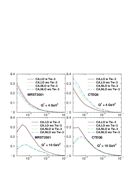
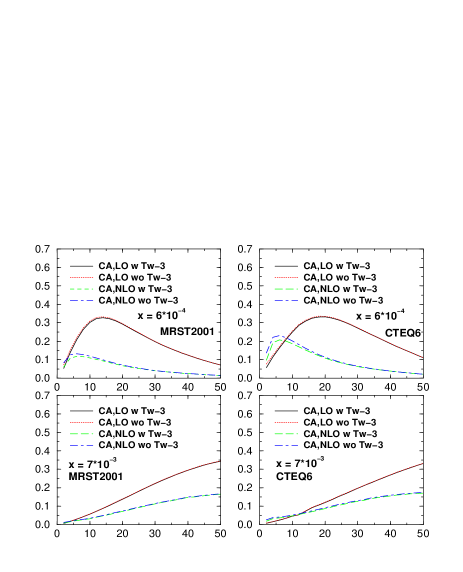
Figure 3: $t$ integrated CA in HERA kinematics vs. $x_{bj}$ for two typical values of $Q^{2}$ and $t_{max}=-0.5~{}\mbox{GeV}^{2}$. W stands for “with” and WO stands for “without”.

Figure 4: $t$ integrated CA in HERA kinematics vs. $Q^{2}$ for two typical values of $x_{bj}$ and $t_{max}=-0.5~{}\mbox{GeV}^{2}$.

As can directly be seen from the Figs. 4 and 4, the twist-3 effect in the CA are entirely negligible at HERA for both the MRST2001 and CTEQ6L LO parameterizations. Furthermore, the two distributions give the same answer within about $10\%$. However, when comparing the respective NLO curves one finds differences of up to $100\%$. They start to disappear for $x_{bj}\to 0.1$ in the given $Q^{2}$ range. For small $x_{bj}$, however, this difference disappears only for $Q^{2}>40~{}\mbox{GeV}^{2}$. This feature was already noted earlier afmmlong in a pure twist-2 analysis and shown to be attributable to the very different NLO gluon distributions at $Q_{0}$. Also note that the exclusion of kinematic power corrections in afmmlong lead to negative numbers for the CA in HERA kinematics in contrast to our findings here. This illustrates the importance of kinematic power corrections for the CA. The NLO corrections, in particular at the smallest $x_{bj}$, are very large and only reduce for the largest $Q^{2}$ to about $100\%$. Again the same was found in a pure twist-2 NLO analysis afmmlong and attributed to a large NLO gluon contribution in the real part of DVCS amplitudes. However, for $x_{bj}>10^{-3}$ and $Q^{2}\geq 10~{}\mbox{GeV}^{2}$ the NLO corrections for CTEQ6M seem to be much smaller than in the case of MRST2001. I will come back to this point when I discuss the SSA. One word has to be said about the influence of the D-term on the CA at this point. Based on the findings about the DVCS amplitudes in afmmamp and by explicit comparison of results with and without a D-term, I conclude that the influence of the D-term is totally negligible for HERA.

Turning now to the SSA, that we can see from Figs. 6 and 6 that the twist-3 effects are even smaller than in the case of the CA. We also see that the room for twist-3 effects in NLO is further reduced compared to the CA. Note that I discuss a positron rather than an electron beam and therefore the sign of the asymmetry is negative.

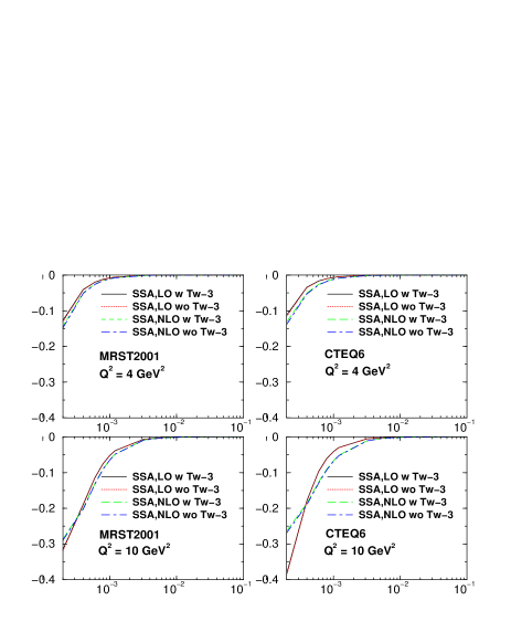
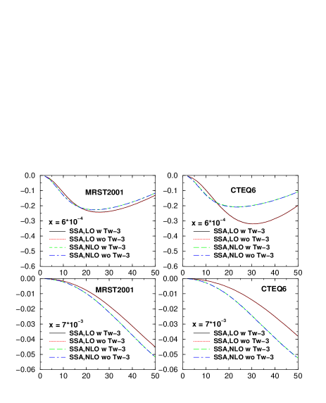
Figure 5: $t$ integrated SSA in HERA kinematics vs. $x_{bj}$ for two typical values of $Q^{2}$ and $t_{max}=-0.5~{}\mbox{GeV}^{2}$. W stands for “with” and WO stands for “without”.

Figure 6: $t$ integrated SSA in HERA kinematics vs. $Q^{2}$ for two typical values of $x_{bj}$ and $t_{max}=-0.5~{}\mbox{GeV}^{2}$.

Furthermore, we see that the NLO corrections are typically of the order of $10-15\%$ but at most $50\%$. This is in agreement with the results found in afmmlong in a pure twist-2 analysis demonstrating that in contrast to the CA, the SSA is quite insensitive to kinematic power corrections. We also see that in NLO both MRST2001 and CTEQ6M give almost identical results, however, differ in LO for large $Q^{2}$ and $x_{bj}<10^{-3}$ which simply illustrates the fact that the LO gluon is larger for CTEQ6L than for MRST2001. In LO, this difference can only manifests itself after a longer evolution path since the DVCS amplitude contains only quarks at leading order. In NLO, where the gluon enters directly on the amplitude level, differences in the gluon manifest themselves at lower $Q^{2}$ in quantities very sensitive to the gluon contribution, like the CA due to its proportionality to the real part. This is well represented when comparing the NLO results for CTEQ6M and MRST2001 in the CA and the SSA at very small $x_{bj}$.

The results for both LO and NLO suggest that both the CA and SSA should be easily measurable with fairly high precision at both the H1 and ZEUS experiment!

IV.2 EIC

In its current design the electron-ion-collider (EIC) will collide $1-10~{}\mbox{GeV}$ electrons from a linear accelerator with $100-250~{}\mbox{GeV}$ unpolarized/polarized protons and unpolarized ions of up to $100~{}\mbox{GeV}$. Note that the projected luminosity for one year at the EIC will be larger than for the entire HERA run, enabling high precision studies of DVCS. For the figures below I chose a center-of-mass energy of $\sqrt{s}=63.25~{}\mbox{GeV}$ which corresponds to a $5~{}\mbox{GeV}$ electron beam and a $200~{}\mbox{GeV}$ proton beam as a sort of average setting for the machine. The $x_{bj}$ range will thus be between roughly $10^{-3}-10^{-1}$. Naturally, the higher $\sqrt{s}$ the closer the kinematics will be to HERA and, thus, also the results. Since we want to investigate the $x_{bj}$ region between HERA and HERMES with an overlap to both experiments, we do not want to go to the highest energies save for cross-checking HERA results. Let me start my discussion with the CA once again and then move on to the SSA. Note that I will apply the same $t$ cuts as in the case of HERA to be able to compare the two settings. Though the proton target can be polarized, I will not discuss such an observable since it was shown in afmmlong that such observables are essentially zero for a collider setting.

As can be seen from Figs. 8 and 8, the twist-3 effects in LO for the CA are at most $10\%$, except at the smallest $x_{bj}$ and lowest $Q^{2}=2~{}\mbox{GeV}^{2}$ where they can reach around $20\%$ and have to be taken into account when trying to extract twist-2 GPDs from the data. In NLO the corrections seem larger but remember that this is only an upper estimate of the actual twist-3 effects in NLO and thus they are not more than $35\%$ at the lowest $x_{bj}$ and $Q^{2}$. It is more likely, however, that they will be of the same size as the LO result or even smaller. Note also that the twist-3 effects quickly vanish for larger $x_{bj}$ within the entire $Q^{2}$ interval, which is mainly a kinematical effect rather than a dynamical one. The two distributions, CTEQ6 and MRST2001, give very similar numbers in LO and at NLO for larger $Q^{2}$, however, differ strongly at low $Q^{2}$ as already seen for the HERA setting. The relative NLO corrections are again large and follow the same pattern for both sets as at HERA. The influence of the D-term on the CA is again negligible.

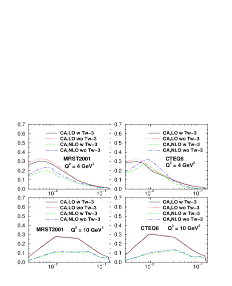
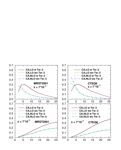
Figure 7: $t$ integrated CA in EIC kinematics vs. $x_{bj}$ for two typical values of $Q^{2}$ and $t_{max}=-0.5~{}\mbox{GeV}^{2}$. W stands for “with” and WO stands for “without”.

Figure 8: $t$ integrated CA in EIC kinematics vs. $Q^{2}$ for two typical values of $x_{bj}$ and $t_{max}=-0.5~{}\mbox{GeV}^{2}$.

When looking at the SSA in Figs. 10 and 10, one notices that the twist-3 effects are basically zero as in the case of HERA and that the NLO corrections are very moderate and of the same size for both sets as in the HERA case. Hence they can be safely neglected in a GPD extraction. Note that the shape of the SSA in $x_{bj}$ and $Q^{2}$ is the mirror of the one at HERA since the EIC uses an electron rather than a positron beam.

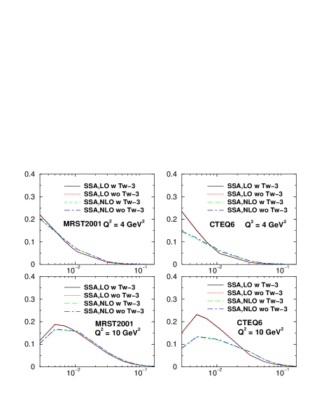
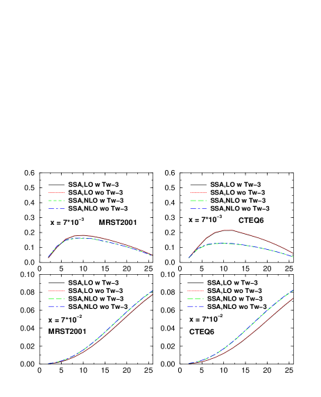
Figure 9: $t$ integrated SSA in EIC kinematics vs. $x_{bj}$ for two typical values of $Q^{2}$ and $t_{max}=-0.5~{}\mbox{GeV}^{2}$. W stands for “with” and WO stands for “without”.

Figure 10: $t$ integrated SSA in EIC kinematics vs. $Q^{2}$ for two typical values of $x_{bj}$ and $t_{max}=-0.5~{}\mbox{GeV}^{2}$.

In conclusion one can say that except at low $Q^{2}$ and the smallest $x_{bj}$ in the CA or a similar asymmetry, the twist-3 effects can be safely neglected and that the size is basically the same as in the case of HERA. These are very encouraging signs that, together with the high luminosity, DVCS will be measured with high precision at the EIC. Therefore, we will be able to reliably extract the leading twist-2 GPD $H$ with high precision in a very broad range of $x_{bj}$ and $Q^{2}$ from the EIC DVCS data!

IV.3 HERMES

In the following I will discuss the fixed-target experiment HERMES with a center-of-mass energy of $\sqrt{s}=7.2~{}\mbox{GeV}$. This allows, broadly speaking, to access a region in $x_{bj}$ of about $0.05-0.3$ with $Q^{2}$ from $1-9~{}\mbox{GeV}^{2}$. HERMES uses the electron/positron beam from HERA with an energy of $E=27.6~{}\mbox{GeV}$. The gas target can be either unpolarized/polarized protons or unpolarized nuclei. I will not discuss observables with a polarized target for HERMES, since there is no clear leading DVCS amplitude, such as $H$ in the case of the CA and SSA, and thus the disentangling of the various contributing GPDs is supremely difficult. In order to allow a comparison with the collider experiments, I once more choose a $t_{max}$ of $-0.5~{}\mbox{GeV}^{2}$ which is also not an unrealistic choice given the fact that the average $t$ for HERMES is about $-0.25~{}\mbox{GeV}^{2}$.

The CA, as can be seen from Figs. 12 and 12, receives larger twist-3 corrections in LO than the CA at HERA or EIC. However, except, at the lowest values of $Q^{2}$ and smallest $x_{bj}$ where they can be as large as factor of $4$, the corrections are generally speaking $15\%$ or less. Note that as $Q^{2}$ increases the twist-3 corrections rapidly disappear in both LO and NLO. The LO results between the two sets agree very nicely but there is quite a difference in NLO. The NLO corrections themselves are again quite large but not larger than at HERA or EIC. In fact, for larger $Q^{2}$ and larger $x_{bj}$ they are quite small. Note that when averaging the LO and NLO results with kinematic power corrections for the CA for both sets over $Q^{2}$ and $x_{bj}$ one obtains the same numbers as in afmmms while the number for LO with full twist-3 is about $0.1$ neatly interpolating between the LO and NLO result of $0.12$ and $0.09$ respectively. This compares very favorably with the experimental HERMES result of $0.11\pm 0.04\pm 0.04$ hermnew for $\langle x\rangle=0.12,\langle Q^{2}\rangle=2.8~{}\mbox{GeV}^{2},\langle t\rangle=-0.27~{}\mbox{GeV}^{2}$. One can see that the averaging process washes out any differences between the two GPD sets, which, however, were not that tremendous to begin with. A word about the D-term and its influence on the CA is in order at this point. Recently gpdlat1 ; gpdlat2 , the first lattice results on the coefficient of the D-term were obtained and found to differ from the prediction of the chiral-quark-soliton model vanderhagen1 quite substantially. The respective calculations were done at different normalization points ($\mu=2~{}\mbox{GeV}$ for the lattice i.e. within HERMES kinematics, and $\mu=0.6~{}\mbox{GeV}$ for the chiral-quark-soliton model). Evolution itself cannot account for the observed difference of about a factor of $4$. When studying the LO and NLO evolution of the D-term using the GRV98 PDF grv98 with the above GPD Ansatz one finds that in both LO and NLO the quark D-term is reduced by about $30\%$ from the respective input scale of $Q_{0}=0.51~{}\mbox{GeV}$ (LO) and $Q_{0}=0.63~{}\mbox{GeV}$ (NLO) to $Q=2~{}\mbox{GeV}$ (the difference between LO and NLO is about $2\%$), leaving still a factor of about $3$ between the two results modulo the uncertainty associated with a gluonic D-term which migh, given the right sign and size, be able to account for the observed difference. GRV98 was used since the input scales are very close to the one of the chiral-quark-soliton model. When studying the importance of the D-term for DVCS observables I find that if the D-term were either omitted or its size reduced by a factor of about $3-4$, the CA would become so small that it would no longer be in good agreement with the data. However, using a different Ansatz for twist-2 GPDs based on a double distribution model (see for example rad1 ) and neglecting evolution effects, the authors of bemu4 describe the CA without a D-term. It was shown in afmmms , though, that this type of double distribution Ansatz as chosen in bemu4 , cannot describe the DVCS data in either LO or NLO when evolution effects are taken into account! The situation will unfortunately remain unresolved until better fixed target data will become available.

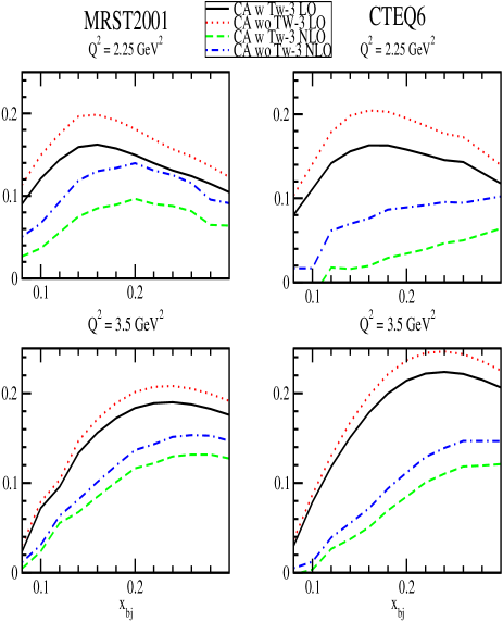
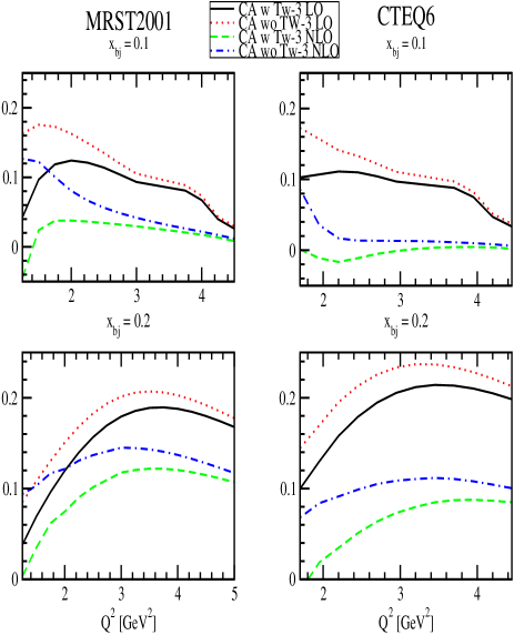
Figure 11: $t$ integrated CA in HERMES kinematics vs. $x_{bj}$ for two typical values of $Q^{2}$ and $t_{max}=-0.5~{}\mbox{GeV}^{2}$. W stands for “with” and WO stands for “without”.

Figure 12: $t$ integrated CA in HERMES kinematics vs. $Q^{2}$ for two typical values of $x_{bj}$ and $t_{max}=-0.5~{}\mbox{GeV}^{2}$.

When turning to the SSA in Figs. 14 and 14, one can see that the twist-3 effects in LO are at most $10\%$ and that the NLO corrections are, as in the case of HERA and EIC, very moderate and at most about $35\%$. The results of the two sets in LO are virtually identical and still within $20\%$ at NLO. When averaged over $Q^{2}$ and $x_{bj}$ the results of the two sets do not differ any longer and reproduce the LO and NLO results of afmmms $-0.28$ and $-0.23$ as they should since the model is the same. This again compares favorably with the experimental result of $-0.21\pm 0.04\pm 0.04$ hermssa for virtually the same average kinematics as the CA.

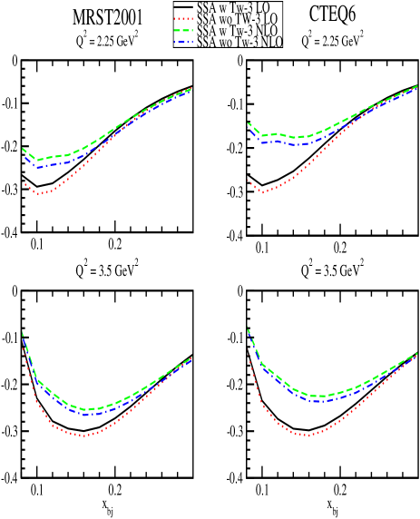
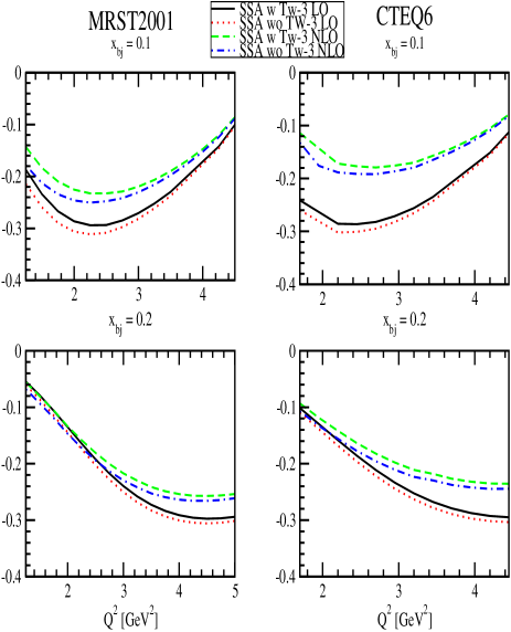
Figure 13: $t$ integrated SSA in HERMES kinematics vs. $x_{bj}$ for two typical values of $Q^{2}$ and $t_{max}=-0.5~{}\mbox{GeV}^{2}$. W stands for “with” and WO stands for “without”.

Figure 14: $t$ integrated SSA in HERMES kinematics vs. $Q^{2}$ for two typical values of $x_{bj}$ and $t_{max}=-0.5~{}\mbox{GeV}^{2}$.

In conclusion, one can say that higher twist effects can be neglected for the SSA at HERMES and thus it can serve as a tool for GPD extraction. The CA is much more sensitive to twist-3 effects, however, they are still small enough that they can be neglected given the accuracy of the data, except for the lowest $Q^{2}$ and $x_{bj}$ values. This implies that for about $Q^{2}>2-2.5~{}\mbox{GeV}^{2}$ the CA can also be used for a GPD extraction or at the very least as a cross check to fits from smaller $x_{bj}$ and the HERMES SSA. The GPD model used in this study already produces very favorable agreement with the SSA and CA data without resorting to a fit and can thus serve as a basis for a successful parameterization.

IV.4 CLAS

The CLAS experiment is a fixed target experiment with very high luminosity but a low center of mass energy. I will first investigate an electron beam of $E=4.3~{}\mbox{GeV}$ and then one with $E=5.75~{}\mbox{GeV}$ corresponding to the energies at the first and second CLAS run respectively. Here I will concentrate on the SSA and omit the CA or a similar asymmetry due to the mentioned difficulties CLAS has or will have with these type of asymmetries as explained in Sec. II. Also, I will only discuss the set of GPDs generated from MRST2001 since the $Q_{0}=1~{}\mbox{GeV}$ is low enough, compared to the one from CTEQ6 of $Q_{0}=1.3~{}\mbox{GeV}$, to have a meaningful range in $x_{bj}$ and $Q^{2}$ for both CLAS settings.

Let us start with the lower energy setting, where I have chosen a $t_{max}=-0.25~{}\mbox{GeV}$ to get as large a range in $x_{bj}$ and $Q^{2}$ as possible. As one can see from Fig. 15 the twist-3 effects in LO are even for such a low energy as CLAS has less than $10\%$ and thus basically negligible! This fits in nicely with the measured twist-3 effect at CLAS clas1 which is about $10\%$ of the measured SSA for the central value but is compatible with zero within the experimental errors. Furthermore, the NLO effects are at most $50\%$ and typically around $20\%$ and thus not as large as one might have feared for such low $Q^{2}$ values. This is mainly due to the fact that the influence of the gluon on the amplitude in NLO at large $x_{bj}$ is not as pronounced as at smaller $x_{bj}$ where its importance grows quickly. Notwithstanding this fact, the usage of perturbation theory at such small $Q^{2}$ remains still questionable on general grounds. However, one can definitely say that the twist-2 handbag contribution to DVCS is the leading contribution to the SSA at CLAS. This alone is quite an amazing statement given that one would naively have expected that at these energies higher twist contributions would be the dominant ones. When averaging over $x_{bj}$ and $Q^{2}$ one obtains a value for the SSA in average CLAS kinematics ($\langle x\rangle=0.19,\langle Q^{2}\rangle=1.31~{}\mbox{GeV}^{2},\langle t\rangle=-0.19~{}\mbox{GeV}^{2}$) of about $0.2$ in LO and about $0.14$ in NLO which is, at least in LO, in good agreement with the experimental value of $0.202\pm 0.021\pm 0.02$ clas1 .

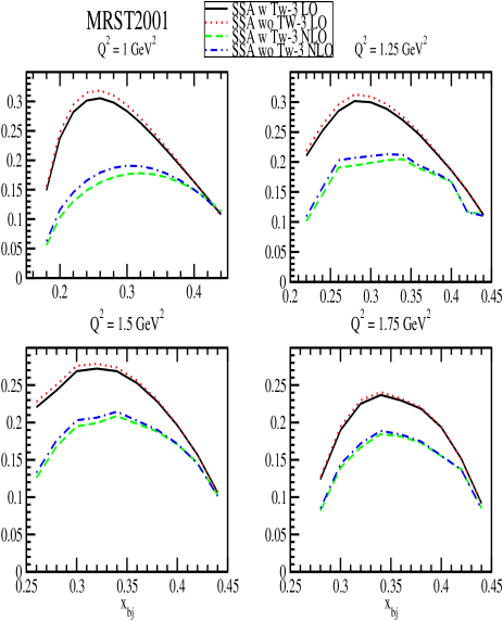
Figure 15: $t$ integrated SSA in CLAS kinematics vs. $x_{bj}$ for four typical values of $Q^{2}$ and $t_{max}=-0.25~{}\mbox{GeV}^{2}$. W stands for “with” and WO stands for “without”.

In the higher energy setting, I have introduced two different $t_{max}$ values, in order to both compare to the lower energy setting and demonstrate how the SSA changes for a drastic change in cut-off for $t$. As can be seen from Figs. 17, 17, 19 and 19 the twist-3 contributions are again very small in both LO and NLO for both cuts in $t$ and are at most $10\%$ which is in agreement with the value at lower energy. The NLO corrections are mostly moderate except for the lowest values of $x_{bj}$ and $Q^{2}$ as seen at lower energies. The distribution in $x_{bj}$ for different $Q^{2}$ between the lower and higher energy setting at the same $t_{max}$ (Figs. 15 and 17) shows the distributions to be very similar both in shape and size. When comparing the different cuts in $t$ for the higher energy setting (Figs. 17 and 17 and Figs. 19 and 19) one notices that the distributions in $x_{bj}$ with the higher $t$ cut are wider and thus flatter than the one for a lower cut in $t$. The maxima of the curves move also to larger values of $x_{bj}$. The $Q^{2}$ distributions are virtually unaltered. There is an overall tendency for the maxima to be somewhat higher for the higher $t$ cut, but only by at most $10\%$.

We thus see that different cuts in $t$ have only a marginal effect in the size and distribution of the SSA. When further averaging over $x_{bj}$ and $Q^{2}$ the sensitivity will be further reduced. In fact, as one can see from the figures, cuts in $x_{bj}$ and $Q^{2}$ will have a much bigger effects than the one in $t$!

Unfortunately, there is no published data yet with which to compare and without knowing the average kinematics, let alone the experimental acceptance, it is impossible to make a sensible prediction at this point.

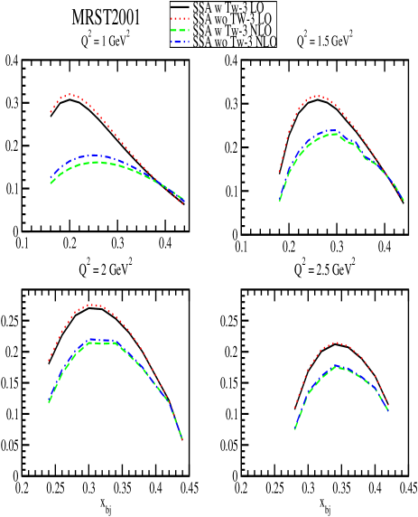
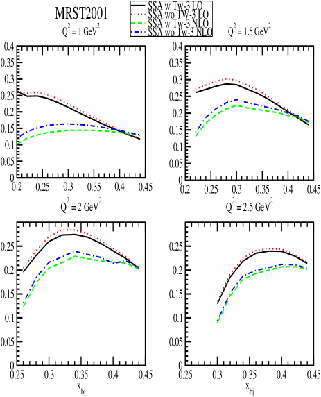
Figure 16: $t$ integrated SSA in CLAS kinematics vs. $x_{bj}$ for four typical values of $Q^{2}$ and $t_{max}=-0.25~{}\mbox{GeV}^{2}$. W stands for “with” and WO stands for “without”.

Figure 17: $t$ integrated SSA in CLAS kinematics vs. $x_{bj}$ for four typical values of $Q^{2}$ and $t_{max}=-0.5~{}\mbox{GeV}^{2}$. W stands for “with” and WO stands for “without”.

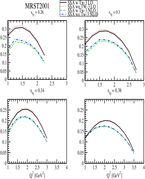
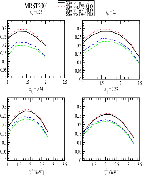
Figure 18: $t$ integrated SSA in CLAS kinematics vs. $Q^{2}$ for four typical values of $x_{bj}$ and $t_{max}=-0.25~{}\mbox{GeV}^{2}$.

Figure 19: $t$ integrated SSA in CLAS kinematics vs. $Q^{2}$ for four typical values of $x_{bj}$ and $t_{max}=-0.5~{}\mbox{GeV}^{2}$.

V Phenomenological parameterization of the GPD $H$

Let me now turn to a sensible, phenomenological parameterization of the $X$, $\zeta$ and $t$ dependence of the leading twist-2 GPD $H$ at a low normalization point $Q_{0}$. First, I will give the parameterization of $H$ in LO and NLO and then justify it based on the available data.

As is clear from the preceding section, the NLO parameterizations seem to work very well in their current form except for CLAS. However, for CLAS the GPD $H$ will not be the leading one anymore as it is for HERA, EIC and HERMES. In fact, the contributions from other GPDs could be set to zero without changing the HERA and only by a few percent the HERMES results. Since I only want to make a statement about $H$, I will restrict myself to a good description of the data from H1, ZEUS and HERMES.

Based on the analysis carried out in afmmms , the MRST2001 NLO PDF parameterization at $Q_{0}=1~{}\mbox{GeV}$ with $\Lambda^{N_{f}=4,NLO}_{QCD}=323~{}\mbox{MeV}$ using the prescriptions of Eqs. (15),(17) and (18) does the best job in describing the DVCS data from H1, ZEUS and HERMES. There is no need to change the NLO parameterization of Sec. III.

The story is different for LO. The LO results using Eqs. (15),(17) and (18) are consistently above the DVCS data save for CLAS. A way to find a LO parameterization giving a good description of the data is to vary the shift parameter $a$ in $\zeta$. The shift parameter is given by the number in front of $\zeta$ in the argument of the forward PDF $(X-a\zeta)/(1-a\zeta)$ i.e. $a=1/2$ in Sec. III. A shift parameter of $a=1/2$ works well for NLO but not for LO. In fact, the best description of the DVCS data in LO is found for $a\simeq 0$ for the MRST2001 LO PDF with $Q_{0}=1~{}\mbox{GeV}$ and $\Lambda^{N_{f}=4,LO}_{QCD}=220~{}\mbox{MeV}$. Note that any $a\neq 1/2$ will violate the “Munich symmetry” of double distributions rad2 ; much1 though still fullfilling all the other requirements. Given the fact that the NLO parameterization fullfills all necessary requirements and, save for absolute numbers, looks the same as the LO parameterization, one can conclude that the LO parameterization is still phenomenologically useful since it describes the data and can be used for good quantitative estimates though it neglects higher order corrections and violates some subtle symmetries.

Let me illustrate this with the example of the H1 data Figs. 20 and 21 for the DVCS $\gamma^{*}$-proton cross section, $\sigma(\gamma^{*}p)$, Eq. (14). As I explained before, the leading DVCS amplitude at small $x_{bj}$ is generated via the GPD $H$. The interference term in the DVCS cross section is, after integration over $\phi$, only a percent contribution to $\sigma(\gamma^{*}p)$. The BH term is usually also negligible compared to the pure DVCS term, however, since we are able to compute it unambiguously to high accuracy, one can simply subtract the BH contribution from the data. In this case the $t$ dependence can be simplified to an exponential form $e^{{\cal B}t}$. For the H1 data it is sufficient to take ${\cal B}$ to be a constant. However, for the ZEUS data this is not sufficient anymore (see afmmms ). Though not necessary, I will use the $Q^{2}$ dependent slope of afmmms

$${\cal B}(Q^{2})={\cal B}_{0}\left(1-C\ln\left(\frac{Q^{2}}{Q_{0}^{2}}\right)\right),$$ (33)

with ${\cal B}_{0}=8~{}\mbox{GeV}^{-2}$, $Q_{0}=2~{}\mbox{GeV}^{2}$, $C=0.15$. The reason for choosing such a parameterization are given in great detail in afmmms and need not be repeated here. A physically intuitive explanation for this behavior of the slope is given in afgpd3d .

As can be easily seen when comparing the upper and lower plots in Figs. 20 and 21, the LO MRST2001 curve now compares very favorably with the H1 data. In fact, it gives virtually the same result as CTEQ6M i.e. it underestimates the ZEUS data somewhat. For the fixed target kinematics it is in agreement with the HERMES data on the SSA ($0.21$) and CA ($0.09$) and the CLAS data ($0.17$) on the SSA when kinematically averaged.

I would like to comment now on the $t$ dependence of GPD $H$ at $Q_{0}$. Note that in the parameterization of the slope ${\cal B}$, I did not introduce a $x_{bj}$ or $W$ dependence as is customarily done (see for example ffs and references therein) to account for cone shrinkage i.e. the fact that the slope increases as $x_{bj}$ decreases for constant $Q^{2}$. However the slope change in $x_{bj}$ for HERA kinematics is only of the order of $10\%$ and can thus be neglected for practical purposes. Furthermore, the necessity of a $Q^{2}$ dependent slope signals a breakdown of factorizing the $t$ from the $X$ and $\zeta$ dependence as has always been done in modeling GPDs. The breakdown at small $x_{bj}$ does not occur until fairly large values of $Q^{2}$ which is very suggestive of the following scenario: At the initial scale $Q_{0}$ one has a factorized component of the $t$ dependence which serves as a normalization and will be different for valence-quarks, sea-quarks and gluons. This difference in normalization between quarks and gluons will change as the gluon mixes with the quark-singlet under perturbative evolution. This change in the normalization will be $Q^{2}$ dependent and thus, the form of Eq. (33) is very natural since evolution resums logs of $Q^{2}$. The $x_{bj}$ dependence of the slope can be generated similarly if the $\zeta$ dependence of the GPD is $\zeta^{-\lambda-\alpha t}$ i.e. a regge-like dependence with $\alpha\simeq 0.25~{}\mbox{GeV}^{-2}$ but possibly smaller, especially for gluons, which will also acquire a logarithmic $Q^{2}$ dependence through evolution much like the logarithmic slope of $F_{2}$ H1f2fit . This type of slope change can also be parameterized with an exponential form as in Eq. (33) with $Q^{2}$ replaced by $W$ i.e. $x_{bj}$. Note that in order to maintain polynomiality of the GPD $H$ for $t\neq 0$, the coefficients $A^{i}(\zeta)$ in Eq. (17) will also acquire a $t$ dependence in order to compensate the extra factor of $\zeta^{-\alpha t}$.

A sensible parameterization for the $t$ dependence of the GPD $H$ at $Q_{0}$ would thus be to choose a factorized exponential part with a square root of the slope of $\frac{1}{2}{\cal B}_{q}\simeq 4-5~{}\mbox{GeV}^{-1}$ for the quark sea and $\frac{1}{2}{\cal B}_{g}\simeq 2-2.5~{}\mbox{GeV}^{-1}$ for the gluon. The valence quarks retain the dipole distribution in $t$ used in this paper. The $t$ dependence in $\zeta$ can then be chosen to be $\zeta^{-\alpha t}$ for the quark sea and the gluon with $\alpha\simeq 0.25~{}\mbox{GeV}^{-2}$ for simplicity. The valence distribution could in principle also have a $\zeta^{-\alpha t}$ behavior but this will be extremely difficult to disentangle from data from small $t$. A more accurate parameterization in $t$ will require much more precise data as can be expected from the EIC.

This completes the phenomenological parameterization of the input GPD $H$ in LO and NLO.

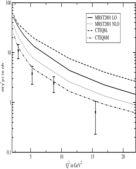
Figure 20: The photon level cross section, $\sigma(\gamma^{*}p\to\gamma p)$, in the average kinematics of the H1 data as a function of $Q^{2}$ at fixed $W=75~{}\mbox{GeV}$ with shift parameter $a=1/2$ (upper plot) and $a=0$ (lower plot).

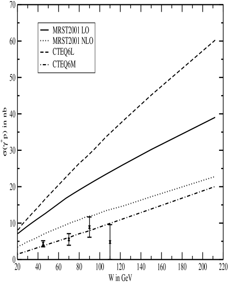
Figure 21: The photon level cross section, $\sigma(\gamma^{*}p\to\gamma p)$, in the average kinematics of the H1 data as a function of $W$ at fixed $Q^{2}=4.5~{}\mbox{GeV}^{2}$ with shift parameter $a=1/2$ (upper plot) and $a=0$ (lower plot).

VI Conclusions

I have given a detailed account of LO twist-3 effects in the WW approximation including their perturbative evolution on DVCS observables for kinematical settings equivalent to the HERA, EIC, HERMES and CLAS experiments. Based on the successful GPD Ansatz of afmmms , I found that the twist-3 effects for the collider settings are negligible save for the lowest values of $Q^{2}$ and $x_{bj}$. For these $Q^{2}$ and $x_{bj}$ values the twist-3 effects still only reach about $10\%$ in observables sensitive to the real part of DVCS amplitudes namely the charge asymmetry and even less in observables sensitive to the imaginary part of DVCS amplitudes such as the single spin asymmetry. The twist-3 effects for the fixed target experiments were only sizeable for the charge asymmetry at low $Q^{2}$ and $x_{bj}$, however not larger than $10-15\%$ for the single spin asymmetry. The common feature, of course, is the virtual disappearance of these effects for $Q^{2}$ values larger than about $3-5~{}\mbox{GeV}^{2}$ depending on the value of $x_{bj}$. The relative smallness of twist-3 effects combined with the fact that twist-3 DVCS amplitudes in the WW approximation are entirely expressible through twist-2 GPDs makes an extraction of at least the unpolarized twist-2 GPD $H$ which is leading in at least three of the four kinematical settings, entirely feasible even with the current, relatively low statistics data. The EIC with its high luminosity will then enable a high precision extraction of the twist-2 GPD $H$.

Since the current data from H1, ZEUS and HERMES are already remarkably restrictive for $H$, I give a first, phenomenological, parameterization, though not a fit, in $X,\zeta$ and $t$ at a low normalization point $Q_{0}$ which describes all available DVCS data from HERA and HERMES in both LO and NLO and from CLAS in LO.

References

- (1) D. Müller et al., Fortschr. Phys. 42, 101 (1994).
- (2) X. Ji, Phys. Rev. D 55 7114 (1997); J. Phys. G 24, 1181 (1998).
- (3) A. V. Radyushkin, Phys. Rev. D 56, 5524 (1997).
- (4) M. Diehl et al., Phys. Lett. B 411, 193 (1997), Eur. Phys. J. C8 409 (1999), Phys. Lett. B428 359 (1998). M. Diehl, Eur. Phys. J. C19 485 (2001).
- (5) M. Vanderhaeghen, P. A. M. Guichon and M. Guidal, Phys. Rev. D 60, 094017 (1999).
- (6) J. C. Collins and A. Freund, Phys. Rev. D 59, 074009 (1999).
- (7) L. Frankfurt et al., Phys. Lett. B 418, 345 (1998), Erratum-ibid. 429, 414 (1998); A. Freund and V. Guzey, Phys. Lett. B 462 178 (1999).
- (8) L. Frankfurt, A. Freund and M. Strikman, Phys. Rev. D 58, 114001 (1998), Erratum-ibid. D 59, 119901 (1999); Phys. Lett. B 460, 417 (1999); A. Freund and M. Strikman, Phys. Rev. D 60, 071501 (1999).
- (9) K. J. Golec-Biernat and A. D. Martin, Phys. Rev. D 59, 014029 (1999).
- (10) A. G. Shuvaev et al., Phys. Rev. D 60, 014015 (1999); K. J. Golec-Biernat, A. D. Martin and M. G. Ryskin, Phys. Lett. B 456, 232 (1999).
- (11) A. V. Belitsky, D. Müller, Phys. Lett. B417, 129 (1998), Nucl. Phys. B537, 397 (1999), Phys. Lett. B464, 249 (1999), Nucl. Phys. B589, 611 (2000), Phys. Lett. B486, 369 (2000), A. V. Belitsky, A. Freund, D. Müller, Phys. Lett. B461, 270 (1999), Nucl. Phys. B574, 347 (2000), Phys. Lett. B493, 341 (2000).
- (12) M. V. Polyakov and A. G. Shuvaev, hep-ph/0207153.
- (13)
- (14) A. Freund, hep-ph/0212017.
- (15) M. Burkardt, Int. J. Mod. Phys. A 18, (2003) 173, Phys. Rev. D62 (2000) 071503, Erratum-ibid.D 66, (2002) 119903.
- (16) M. Diehl, Eur. Phys. J. C25 (2002) 223.
- (17) A. V. Belitsky and D. Müller, Nucl. Phys. A 711 (2002) 118.
- (18) Xiang-dong Ji, hep-ph/0304037.
- (19) Regular parton distributions are merely particle distributions not particle correlation functions.
- (20) A. V. Belitsky and D. Müller, Nucl. Phys. B 589 (2000), 611.
- (21) A. V. Radyushkin and C. Weiss, Phys. Lett. B 493 (2000) 332, Phys. Rev. D 63 (2001) 114012.
- (22) I. V. Anikin, B. Pire and O. V. Teryaev, Phys. Rev. D 62 (2000) 071501.
- (23) N. Kivel and M. V. Polyakov, Nucl. Phys. B 600, (2001) 334.
- (24) N. Kivel and L. Manchiewicz, hep-ph/0305207.
- (25) A. Freund and M. McDermott, Phys. Rev. D 65, 091901 (2002).
- (26) A. Freund and M. McDermott, Eur. Phys. J. C 23, 651 (2002).
- (27) A. V. Belitsky et al., Nucl. Phys. B 593, 289 (2001).
- (28) A. V. Belitsky, D. Müller and A. Kirchner, Nucl. Phys. B 629, 323 (2002).
- (29) N. Kivel, M. V. Polyakov and M. Vanderhaeghen, Phys. Rev. D 63, 114014 (2001).
- (30) A. Freund and M. McDermott, Phys. Rev. D 65, 074008 (2002).
- (31) A. Freund and M. McDermott, Phys. Rev. D 65, 056012 (2002).
- (32) A. Freund, M. McDermott and M. Strikman, Phys. Rev. D67, 036001 (2003).
- (33) L. Frankfurt and M. Strikman, Phys. Rept. 160, 235 (1988); Nucl. Phys. B 316, 340 (1989).
- (34) The first moment counts the number of quarks in the proton and the second moment is a generalization of the momentum sum rule where the D-term generates all the deviation from unity as varies.
- (35) A. V. Radyushkin, Phys. Rev. D 59, 014030 (1999).
- (36) A. V. Radyushkin, Phys. Lett. B 449, 81 (1999).
- (37) M. V. Polyakov and C. Weiss, Phys. Rev. D 60, 114017 (1999).
- (38) B. Pire, J. Soffer and O. Teryaev, Eur. Phys. J. C8 103 (1999).
- (39) P. V. Pobylitsa, hep-ph/0211160, Phys. Rev. D67 (2003) 034009, Phys. Rev. D65 (2002) 114015, Phys. Rev. D65 (2002) 077504.
- (40) A. D. Martin et al., Eur. Phys. J. C 23, 73 (2002).
- (41) J. Pumplin et al., CTEQ Collaboration, J. High Energ. Phys. 0207, 012 (2002).
- (42) M. Glück et al., Phys. Rev. D63 (2001) 094005.
- (43) K. Göcke, M. V. Polyakov and M. Vanderhaeghen, Prog. Part. Nucl. Phys. 47 (2001) 401.
- (44) CLAS Collaboration, S. Stepanyan et al., Phys. Rev. Lett. 87, 182002 (2001);
- (45) ZEUS Collaboration, P. R. Saull, hep-ex/0003030, ZEUS Collaboration, hep-ex/0305028.
- (46) H1 Collaboration, C. Adloff et al., Phys. Lett. B 517, 47 (2001).
- (47) http://www-spires.dur.ac.uk/hepdata/dvcs.html.
- (48) F. Ellinghaus, HERMES Collaboration, Nucl. Phys. A 711, 171 (2002).
- (49) M. Göckeler, R. Horsley, D. Pleiter, P. E. L. Rakow, A. Schäfer, G. Schierholz and W. Schroers, hep-ph/0304249.
- (50) P. Hägler, J. Negele, D. Renner, W. Schroers, T. Lippert and K. Schilling, hep-lat/0304018.
- (51) M. Glück, E. Reya and A. Vogt, Eur. Phys. J. C 5, 461 (1998).
- (52) HERMES Collaboration, Phys. Rev. Lett. 87, 182001(2001).
- (53) L. Mankiewicz, G. Piller and T. Weigl, Eur. Phys. J. C5, 119 (1998)
- (54) H1 Collaboration, Eur. Phys. J. C 21, 33 (2001).