On contributions of fundamental particles to the vacuum energy

Abstract

Recently different regularization schemes for calculations of the vacuum energy stored in the zero-point motion of fundamental fields were discussed. We show that the contribution of the fermionic and bosonic fields to the energy of the vacuum depends on the physical realization of the vacuum state. The energy density of the homogeneous equilibrium vacuum is zero irrespective of the fermionic and bosonic content of the effective theories in the infra-red corner. The contribution of the low-energy fermions and bosons becomes important when the coexistence of different vacua is considered, such as the bubble of the true vacuum inside the false one. We consider the case when these vacua differ only by the masses of the low-energy fermionic fields, $M_{\rm true}>M_{\rm false}$, while their ultraviolet structure is identical. In this geometry the energy density of the false vacuum outside the bubble is zero, $\rho_{\rm false}=-P_{\rm false}=0$, which corresponds to zero cosmological constant. The energy density of the true vacuum inside the bubble is $\rho_{\rm true}=-P_{\rm true}\propto-\Lambda^{2}(M^{2}_{\rm true}-M^{2}_{\rm false})$, where $\Lambda$ is the ultraviolet cut-off.

1 Introduction

Recently the problem of the contribution of different fermionic and bosonic fields to the vacuum energy was revived in relation to the cosmological constant problem (see e.g. [1, 2]). The general form of the vacuum energy density under discussion was

$$\rho=a_{4}\Lambda^{4}+a_{2}\Lambda^{2}M^{2}+a_{0}M^{4}\ln{\Lambda^{2}\over M^{2}}~{},$$ (1)

where $M$ is the mass of the corresponding field, and $\Lambda$ is the ultraviolet energy cut-off. Different regularization schemes were suggested in order to obtain the dimensionless parameters $a_{i}$.

Here we consider this problem from the point of view of the effective relativistic quantum field theory emergent in the low-energy corner of the quantum vacuum, whose ultraviolet structure is known. It appears that the parameters $a_{i}$ depend on the details of the trans-Planckian physics. But in addition we find that even if the two vacua have completely identical structure throughout all the scales, the parameters $a_{i}$ depend on the arrangement and geometry of the vaccum state. In particular, if the vacuum is completely homogeneous and static, all the parameters vanish, $a_{4}=a_{2}=a_{0}=0$, which corresponds to zero cosmological constant. While in the presence of the interface between two different vacua, the energy density can depend not only on the mass $M$, but also on the mass of the quantum field in the neighboring vacuum.

As an example we consider two vacua, whose structure is identical in the high-energy limit, while in the low-energy corner they have the same fermionic content, but their low-energy fermions have slightly different masses. Let us assume that both vacua correspond to the local minima, and the route between these vacua lies only through the vacuum with Weyl fermions of zero mass. Then these vacua can coexist in the configuration shown in Fig. 1. The false vacuum occupies the whole Universe except for the bubble of the true vacuum separated from the false vacuum by the interface where the vacuum has zero-mass fermions. Let us consider the behavior of the vacuum energy density $\rho$ outside and inside the bubble, when this confiuration is static, i.e. when the bubble has the critical size $R$ corresponding to the saddle point of energy functional.

The picture, which is supported by the effective relativistic quantum field theory emerging in condensed matter systems, where the structure of the vacuum is known both at high and low energy (Sec. 2), is shown in Fig. 1. The energy density of the false vacuum outside the bubble does not contain any fermionic mass $M$, since this energy is simply zero;

$$\rho_{\rm false}=-P_{\rm false}=0~{}.$$ (2)

This corresponds to zero cosmological constant in any homogeneous vacuum, if the vacuum is stationary, corresponds to the extremum of the energy functional, and is isolated from the environment [3].

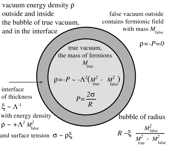
Figure 1: Critical bubble of true vacuum inside the false one.

The energy density of the true vacuum inside the bubble,

$$\rho_{\rm true}=-P_{\rm true}\sim-\Lambda^{2}\left(M_{\rm true}^{2}-M_{\rm false}^{2}\right)\sqrt{-g}<0~{}.$$ (3)

contains the quadratic in $M_{\rm true}$ term with negative sign, but it also depends quadratically on the fermionic mass $M_{\rm false}$ in the neighboring vacuum. On the other hand, if the true vacuum occupies the whole space and becomes equilibrium, its vacuum energy density is zero again, $\rho_{\rm true}=-P_{\rm true}=0$.

All this can be obtained without invoking the microscopic (ultraviolet) structure of the quantum vacuum, using only the general arguments of the vacuum stability. However, here we shall use the microscopic model from which the relativistic quantum field theory with massive fermions emerges in the low-energy corner.

2 Vacuum energy in effective quantum field theory

2.1 Effective quantum field theory with Dirac fermions

Massive relativistic fermions are realized as the low-energy Bogoliubov quasiparticles in the class of the spin-triplet superfluids/superconductors (see section 7.4.9 of [3]). The Bogoliubov–Nambu Hamiltonian for fermionic quasiparticles (analog of elementary particles) is the $4\times 4$ matrix

$$H_{\bf p}=\check{\tau}^{3}\left({p^{2}\over 2m}-\mu\right)+\check{\tau}^{1}\sigma^{\mu}p_{i}~{}e_{\mu}^{i}~{},$$ (4)

$$e_{\mu}^{i}={\Lambda\over p_{F}}\left(\hat{x}_{\mu}\hat{x}^{i}+\hat{y}_{\mu}\hat{y}^{i}\right)+{M\over p_{F}}\hat{z}_{\mu}\hat{z}^{i}~{}~{},~{}~{}{p_{F}^{2}\over 2m}=\mu~{}.$$ (5)

Here $\mu$ is the chemical potential of the particles (atoms) forming the liquid (analog of the quantum vacuum); $m$ is their mass; $\check{\tau}^{a}$ and $\sigma^{\mu}$ are $2\times 2$ Pauli matrices describing the Bogoliubov-Nambu spin and the ordinary spin of particles correspondingly; $\Lambda$ and $M$ are amplitudes of the order parameter $e_{\mu}^{i}$.

One should not confuse particles which form the vacuum (atoms of the liquid) and quasiparticles – excitations above the vacuum – which form the analog of matter in quantum liquids and correspond to elementary particles. Quasiparticles do not scatter on the atoms of the liquid if the liquid is in its ground state, and thus for quasiparticles the ground state of the liquid is seen as an empty space – the vacuum – though this space is densly filled by atoms.

The energy spectrum of quasiparticles in this model is

$$E^{2}({\bf p})=H_{\bf p}^{2}=\left({p^{2}\over 2m}-\mu\right)^{2}+\Lambda^{2}{p_{x}^{2}+p_{y}^{2}\over p_{F}^{2}}+M^{2}{p_{z}^{2}\over p_{F}^{2}}~{}.$$ (6)

The case $M=0$ corresponds to the so-called planar phase, while $M=\Lambda$ describes the isotropic B-phase of superfluid ³He.

We assume that the interaction of atoms in the liquid (or electrons in superconductors), which leads to the formation of the order parameter, is such that the locally stable vacuum states of the liquid have $M\ll\Lambda$. Then in the low-energy limit the Bogoliubov–Nambu Hamiltonian for quasiparticles transforms to the Dirac Hamiltonian

$$H_{\bf p}\approx c_{\parallel}\tilde{p}_{z}\check{\tau}^{3}+\check{\tau}^{1}(c_{\perp}p_{x}\sigma_{x}+c_{\perp}p_{y}\sigma_{y}+M\sigma_{z})~{},$$ (7)

$$\tilde{p}_{z}=p_{z}-p_{F}~{}~{},~{}~{}c_{\parallel}={p_{F}\over m}~{}~{},~{}~{}c_{\perp}={\Lambda\over p_{F}}~{},$$ (8)

with the relativistic spectrum

$$E^{2}({\bf p})\approx g^{ik}\tilde{p}_{i}\tilde{p}_{k}+M^{2}~{},$$ (9)

$$\tilde{\bf p}={\bf p}-p_{F}\hat{\bf z}~{}~{},~{}~{}g^{xx}=g^{yy}=c_{\perp}^{2}~{}~{},~{}~{}g^{zz}=c_{\parallel}^{2}~{}.$$ (10)

Here $c_{\parallel}$ is the ‘speed of light’ propagating along the $z$-axis, while in transverse direction the ‘light’ propagates with the speed $c_{\perp}$. Though in this model the effective speed of light depends on the direction of propagation, this anisotropy can be removed by rescaling along the $z$-axis. The speed of light is not fundamental, since it is determined by the material parameters of the microscopic system. However, it is fundamental from the point of view of all inner observers who consist of the low-energy quasiparicles. For them the speed of light does not depend on direction, and they believe in the laws of special relativity since these laws can be confirmed by all experiments (including the Michelson–Morley measurements of the speed of light) which use clock and rods made of the low-energy quasiparticles. The high-energy observer will not agree with that: for us the original model (4) has no Lorentz invariance, and the speed of light is anisotropic.

After rescaling along the $z$-axis the quasiparticles become the complete analog of the Standard Model fermions with mass $M$: the left-handed and right-handed chiral quasiparticles of the planar state with $M=0$ are hybridized to form the Dirac particles with the mass $M$. Note, that together with the effective Dirac fermions, also the effective gravity and effective $U(1)$ and $SU(2)$ gauge fields (with ‘photons’ and ‘gauge bosons’) emerge in the low-energy corner of this model, with all the accompaning phenomena, such as chiral anomaly, running couplings, etc. [3]. The reason for such close analogy is the momentum space topology of the quantum vacuum, which is common for the ground state of the considered liquid and for the quantum vacuum of the Standard Model. The parameter $\Lambda$ plays the role of the Planck energy scale in the effective theory.

2.2 Vacuum energy

This model can serve for the consideration of the contribution of the Dirac fermions to the energy density of the vacuum in equilibrium. In the many body system (superfluid liquid which contain many particles) the relevant vacuum energy whose gradient expansion gives rise to the effective quantum field theory for quasiparticles at low energy is $\left<{\cal H}-\mu{\cal N}\right>_{\rm eq~{}vac}$, [4] where ${\cal H}$ is the Hamiltonian of the system, ${\cal N}$ is the particle number operator for atoms forming the liquid, and $\mu$ is their chemical potential. The energy density of the superfluid/superconducting ground state (analog of the quantum vacuum) with the order parameter $e_{\mu}^{i}$ is given by (see e.g. Eq.(5.38) in [5])

$$\rho={1\over V}\left<{\cal H}-\mu{\cal N}\right>_{\rm vac}={1\over V}\left<{\cal H}-\mu{\cal N}\right>_{{\rm vac}~{}e_{\mu}^{i}=0}-{p_{F}^{3}m\over 12\pi^{2}\hbar^{3}}e_{\mu}^{i}e_{\mu}^{i}~{},$$ (11)

where $V$ is the volume of the system. For the order parameter (5) which gives rise to the relativistic fermions at low energy one has

$$\rho=\rho(0)-{\sqrt{-g}\over 12\pi^{2}\hbar^{3}}\left(2\Lambda^{4}+\Lambda^{2}M^{2}\right)~{},$$ (12)

where $\sqrt{-g}=c_{\parallel}^{-1}c_{\perp}^{-2}$ according to Eq.(10); and $\rho(0)\equiv\rho(e_{\mu}^{i}=0)$ is the energy density in the normal (non-superfluid) state of the liquid, in which $e_{\mu}^{i}=0$. The equation (12) demonstrates that the amplitude $\Lambda$ in the order parameter expression (5) is the proper ultraviolet cut-off for the estimation of the vacuum energy related to the effective relativistic fermions, while the contribution $\rho(0)$, which does not depend on $\Lambda$ and $M$, comes from the more fundamental physics of the normal state of the liquid at energies well above the energy scales $\Lambda$ and $M$. In this model the term $M^{4}\ln(\Lambda^{2}/M^{2})$ is absent, though it naturally appears in all the regularization schemes discussed in [1, 2].

The dimensionless factors in front of $\Lambda^{4}$ and $\Lambda^{2}M^{2}$ were obtained using the microscopic model in Eqs. (5) and (6). In principle, the low-energy fermions in Eq.(9) can be obtained from different microscopic theories, and one finds that the dimensionless factors in front of $\Lambda^{4}$ and $\Lambda^{2}M^{2}$ depend on the details of the Planck physics. In other words, they depend on the regularization imposed by the ultraviolet physics, which cannot be found within the effective low-energy theory.

It is rather natural to think that the equation (12) reflects the general structure (1) of the vacuum energy in terms of the massive fields discussed in [1, 2]. Moreover, from the point of view of the low-energy observers who are made of quasiparticles and live in the liquid and for whom the effective theory is fundamental, the cosmological constant in their world must have the natural value of order $\Lambda^{4}$. However, this is not so. The vacuum energy contains the contribution $\rho(0)$ from the vacuum degrees of freedom with energies well above $\Lambda$ and $M$. Together with the sub-Planckian modes these high-energy modes determine the behavior of the whole vacuum, and in particular the stability of the static vacuum configurations. If something happens in the low-energy corner, so that the vacuum configuration changes, the high-energy degrees of freedom respond to restore the stability of the whole vacuum in the new configuration. As a result $\rho(0)$ is tuned to the low-energy degrees of freedom and thus becomes dependent on $\Lambda$ and $M$ after the adjustment of the trans-Planckian degrees to the sub-Planckian ones. This dependence is different for different realizations of the equilibrium vacuum state. Moreover, the adjustment can cancel completely or almost completely the low-energy contributions. Below we consider how this occurs in the geometry of Fig. 1.

2.3 Energy density of the false vacuum

Let us assume now that the situation is similar to that of the Ising ferromagnet in applied small magnetic field which slightly discriminates between spin-up and spin-down vacua. This means that there are two vacuum states, false and true, corresponding to two nearly degenerate local minima whose fermionic masses are almost the same:

$$0<M^{2}_{\rm true}-M^{2}_{\rm false}\ll M^{2}_{\rm true}\ll\Lambda^{2}~{}.$$ (13)

Then we can apply this to the vacuum states in the geometry of Fig. 1, where the false vacuum is separated by the domain wall (the interface) from the spherical domain containing the true vacuum.

Let us start with the external domain occupied by the false vacuum. This domain is open and it occupies the whole space except for the finite volume. That is why one can apply to this domain the results known for the infinite homogeneous vacuum. First, we note that any equilibrium macroscopic system consisting of the identical elements (atoms in the case of quantum liquids) obeys the Gibbs-Duhem relation

$$E-\mu N-TS=-PV~{},$$ (14)

where $P$ is the pressure and $S$ the entropy (see Chapter 10.9 in Ref. [6]). Applying this to the equilibrium ground state of the system at $T=0$ (the quantum vacuum), one has for the energy density of the vacuum:

$$\rho={1\over V}\left<{\cal H}-\mu{\cal N}\right>_{\rm vac}={E-\mu N\over V}=-P~{}.$$ (15)

This equation of state, $\rho=-P$, is valid for any homogeneous vacuum irrespective of whether the system is relativistic or not. If the effective relativistic quantum field theory emerges in the low-energy corner of the system, this $\rho$ becomes the cosmological cosntant in the low-energy world.

Second, if the system (the Universe) is isolated from the environment, the external pressure $P_{\rm external}=0$. Thus for the false vacuum in Fig. 1 one has $P_{\rm false}=P_{\rm external}=0$, which gives the vanishing energy density of the false vacuum in this geometry:

$$\rho_{\rm false}=-P_{\rm false}=0~{}.$$ (16)

Thus the cosmological constant in the vacuum outside the bubble is zero. This property does not depend on the low-energy physics, and is determined by the physics of the whole vacuum including the degrees of freedom at energies well above the scales $\Lambda$ and $M$. These high-energy degrees of freedom respond to any change in the low-energy corner exactly compensating the contribution from the low-energy degrees of freedom to ensure the zero value of the cosmological constant in the equilibrium homogeneous vacuum.

2.4 Energy and pressure of the true vacuum

Now let us turn to the inner domain occupied by the true vacuum. If the domain is big enough, $R\gg\Lambda^{-1}$, the vacuum can be considered as homogeneous, and thus the equation of state $\rho=-P$ in (15) is applicable. However, this vacuum is not isolated from the environment, and as a result its vacuum energy density is non-zero. This energy density $\rho_{\rm true}$ can be found by comparison with the energy density of the false vacuum using Eq.(12). Since $\rho_{\rm false}=0$ one has

$$\rho_{\rm true}=-P_{\rm true}=\rho_{\rm true}-\rho_{\rm false}=-{1\over 12\pi^{2}\hbar^{3}}\sqrt{-g}\Lambda^{2}\left(M^{2}_{\rm true}-M^{2}_{\rm false}\right)<0~{}.$$ (17)

In this geometry, the true vacuum has the negative cosmological constant proportional to the difference of $M^{2}$ in two vacua. The quartic term $\propto\Lambda^{4}$ does not appear in the considered model; it appears if the two vacua have different physics at energies below $\Lambda$. Note that if the true vacuum is outside and is in equilibrium, the cosmological constant in this vacuum will be zero again.

Let us now estimate the radius $R$ of the static bubble – the saddle-point critical bubble – which is obtained when the vacuum pressure inside the bubble is compensated by the effect of the surface tension. Since the external pressure is zero, the pressure $P_{\rm true}$ within the domain is determined by the surface tension and the curvature of the domain wall:

$$P_{\rm true}=P_{\rm true}-P_{\rm false}={2\sigma\over R}~{}.$$ (18)

Comparing equations (17) and (18) one obtains the radius of the static bubble critical bubble. The order of magnitude of the surface tension is $\sigma\sim\rho(M=0)\xi$, where $\xi$ is the thickness of the domain wall; and $\rho(M=0)$ is the energy density of the vacuum with massless fermions. This energy can be obtained by comparing it with the energy density of either of the domains, and it appears to be positive:

$$\rho(M=0)=\rho(M=0)-\rho_{\rm false}={\sqrt{-g}\over 12\pi^{2}\hbar^{3}}\Lambda^{2}M^{2}_{\rm false}>0~{}.$$ (19)

This gives the following estimation for the radius of the critical bubble:

$$R\sim\xi{M^{2}_{\rm false}\over M^{2}_{\rm true}-M^{2}_{\rm false}}\gg\xi~{}.$$ (20)

Here $\xi\sim\hbar c_{\parallel}/\Lambda$ in our model, and $\xi\sim\hbar c/\Lambda$ in its relativistic counterpart.

3 Conclusion

In general, the energy density of the quantum vacuum is determined by all the vacuum degrees of freedom. They act coherently as the elements of the same medium, which results in the zero value of the cosmological constant if the vacuum is equilibrium, homogeneous and is isolated from the environment. Thus the contribution of the zero-point motion of the low-energy fermionic and bosonic fields to the vacuum energy cannot be singled out from the ultrviolet contributions and thus it cannot be obtained from the low-energy theory by any regularization scheme. The low-energy physics is capable to describe only the contribution of different ifrared perturbations of the vacuum to the vacuum energy density, such as dilute matter, space curvature, expansion of the Universe, rotation, Casimir effect, etc. [3, 7]. This gives rise to induced vacuum energy which is proportional to the energies of the infrared perturbations, including the energy density of matter, which is in agreement with observations [8]. If the Universe evolves in time, cosmological ‘constant’ becomes an evolving physical quantity, which responds to the combined action of the evolving perturbations of the vacuum state.

The example which we considered here is somewhat similar to the Casimir effect, where the difference in energy density between two neghbouring vacua, in the restricted and unrestricted domains, are calculated using the low-energy physics. In our case, the two vacua across the interface (domain wall) also have identical ultraviolet (microscopic) structure and also have very close low-energy theories, whose fermionic and bosonic contents are the same, but the masses of the fields are slightly different. That is why, for the estimation of the difference one can try to explore the low-energy physics. One can use, for example, the regularized equation for the contribution of the massive quantum field to the energy-momentum tensor of the vacuum – the equation (9) in Ref. [1] with minus sign when applied to the fermionic field:

$$t_{\mu\nu}=-g_{\mu\nu}M^{2}\int{d^{4}p\over(2\pi)^{3}}\delta(p^{2}-M^{2})\theta(p_{0})~{}.$$ (21)

Then for the difference in energy and pressure between the true and false vacua one obtains:

$$\rho_{\rm true}-\rho_{\rm false}=P_{\rm false}-P_{\rm true}$$ (22)

$$=-\left(M_{\rm true}^{2}-M^{2}_{\rm false}\right)\int{d^{3}p\over 2(2\pi)^{3}}{1\over cp}\sim-\sqrt{-g}\Lambda^{2}\left(M^{2}_{\rm true}-M^{2}_{\rm false}\right),$$ (23)

where $\sqrt{-g}=c^{-3}$. This gives for the energy and pressure difference the correct dependence on masses, the correct sign and even the correct Gibbs-Duhem relation $\Delta\rho=-\Delta P$. However, the numerical factor is still missing because of the quadratic divergence, and this factor depends on details of the microscopic physics. This demonstrates that the regularization schemes are not applicable in a strict sense even when the difference in the vacuum energies is calculated.

As for the energy density itself (the cosmological constant), it is determined (as in the case of the Einstein and Gödel Universes [7]) by the equilibrium properties of the whole system and depends on the geometry. In particular, for the equilibrium homogeneous vacuum one obtains $\rho=-P=0$, irrespective of whether this vacuum is true or false, and whether it contains massive or massless fermions. On the other hand, the vacuum inside the bubble is not isolated from the environment, as a result the energy density of this vaccum is non-zero and is given by the difference of the quadratic terms in Eq.(3). Except for the numerical factor, this result can be reproduced without consideration of the microscopic theory. In addition to the general arguments of the vacuum stability, including the Gibbs-Duhem relation, one can use the effective low-energy theory for the order-of-magnitude estimation of the energy and pressure difference of two neighboring vacua. For our particular problem, we can use the regularization presented in Eq.(21).

This work was supported by ESF COSLAB Programme and by the Russian Foundations for Fundamental Research.

References

- [1] G. Ossola and A. Sirlin, Considerations concerning the contributions of fundamental particles to the vacuum energy density, hep-ph/0305050.
- [2] E. Kh. Akhmedov, Vacuum energy and relativistic invariance, hep-th/0204048.
- [3] G.E. Volovik, The Universe in a Helium Droplet, Clarendon Press, Oxford (2003).
- [4] A.A. Abrikosov, L.P. Gorkov and I.E. Dzyaloshinskii, Quantum Field Theoretical Methods in Statistical Physics, Pergamon, Oxford (1965).
- [5] V.P. Mineev and K.V. Samokhin, Introduction to Unconventional Superconductivity, Gordon and Breach Science Publishers (1999).
- [6] B. Yavorsky and A. Detlaf, Handbook of Physics, Mir Publishers, Moscow (1975).
- [7] G. E. Volovik, Phenomenology of effective gravity, gr-qc/0304061.
- [8] A. G. Riess, et al., Astron. J. 116, 1009 (1998); S. Perlmutter, et al., Astrophys. J. 517, 565 (1999).