Three-Neutrino Mixing after the First Results from K2K and KamLAND

Abstract

We analyze the impact of the data on long baseline $\nu_{\mu}$ disappearance from the K2K experiment and reactor $\bar{\nu}_{e}$ disappearance from the KamLAND experiment on the determination of the leptonic three-generation mixing parameters. Performing an up-to-date global analysis of solar, atmospheric, reactor and long baseline neutrino data in the context of three-neutrino oscillations, we determine the presently allowed ranges of masses and mixing and we consistently derive the allowed magnitude of the elements of the leptonic mixing matrix. We also quantify the maximum allowed contribution of $\Delta m^{2}_{21}$ oscillations to CP-odd and CP-even observables at future long baseline experiments.

I Introduction

Neutrino oscillations are entering in a new era in which the observations from underground experiments obtained with neutrino beams provided to us by Nature – either from the Sun or from the interactions of cosmic rays in the upper atmosphere– are being confirmed by experiments using “man-made” neutrinos from accelerators and nuclear reactors.

Super–Kamiokande (SK) high statistics data skatmlast ; skatmpub clearly established that the observed deficit in the $\mu$-like atmospheric events is due to the neutrinos arriving in the detector at large zenith angles, strongly suggestive of the $\nu_{\mu}$ oscillation hypothesis. This evidence was also confirmed by other atmospheric experiments such as MACRO macro and Soudan 2 soudan . Similarly, the SNO results snoccnc in combination with the SK data on the zenith angle dependence and recoil energy spectrum of solar neutrinos sksollast and the Homestake chlorine , SAGE sage , GALLEX+GNO gallex ; gno and Kamiokande kamiokande experiments, put on a firm observational basis the long–standing problem of solar neutrinos snp , establishing the need for $\nu_{e}$ conversions.

The KEK to Kamioka long-baseline neutrino oscillation experiment (K2K) uses an accelerator-produced neutrino beam mostly consisting of $\nu_{\mu}$ with a mean energy of 1.3 GeV and a neutrino flight distance of 250 km to probe the same oscillations that were explored with atmospheric neutrinos. Their results k2kprl show that both the number of observed neutrino events and the observed energy spectrum are consistent with neutrino oscillations with oscillation parameters consistent with the ones suggested by atmospheric neutrinos.

The KamLAND experiment measures the flux of $\bar{\nu}_{e}$’s from nuclear reactors with a energy of $\sim$ MeV located at typical distance of $\sim$ 180 km with the aim of exploring with a terrestrial beam the region of neutrino parameters that is relevant for the oscillation interpretation of the solar data. Their first published kamland results show that both the total number of events and their energy spectrum can be better interpreted in terms of $\bar{\nu}_{e}$ oscillations with parameters consistent with the the LMA solar neutrino solution  kamland ; oursolar ; ourkland ; othersolkam .

Altogether, the data from solar and atmospheric neutrino experiments, and the first results from KamLAND and K2K constitute the only solid present–day evidence for physics beyond the Standard Model review . The minimum joint description of these data requires neutrino mixing among all three known neutrinos and it determines the structure of the lepton mixing matrix MNS which can be parametrized as PDG

$$U=\left(\begin{array}[]{ccc}c_{13}c_{12}&s_{12}c_{13}&s_{13}\,{e}^{-i\delta}\\ -s_{12}c_{23}-s_{23}s_{13}c_{12}\,{e}^{i\delta}&c_{23}c_{12}-s_{23}s_{13}s_{12}\,{e}^{i\delta}&s_{23}c_{13}\\ s_{23}s_{12}-s_{13}c_{23}c_{12}\,{e}^{i\delta}&-s_{23}c_{12}-s_{13}s_{12}c_{23}\,{e}^{i\delta}&c_{23}c_{13}\end{array}\right)\,,$$ (1)

where $c_{ij}\equiv\cos\theta_{ij}$ and $s_{ij}\equiv\sin\theta_{ij}$. In addition to the Dirac-type phase, $\delta$, analogous to that of the quark sector, there are two physical phases associated to the Majorana character of neutrinos, which however are not relevant for neutrino oscillations majophases and will be set to zero in what follows.

In this paper we present the result of the global analysis of solar, atmospheric, reactor and long-baseline neutrino data in the context of three-neutrino oscillations with the aim of determining in a consistent way our present knowledge of the leptonic mixing matrix and the neutrino mass differences. We make particular emphasis on the impact of the first data from long baseline $\nu_{\mu}$ disappearance from the K2K experiment and reactor $\bar{\nu}_{e}$ disappearance from the KamLAND experiment.

The outline of the paper is as follows. In Sec. II we describe the data included in the analysis and we briefly describe the relevant formalism. Sec. III.1 contains the results of the analysis of the K2K data and their effect on the determination of the parameters associated with atmospheric oscillations. We find that the main impact of K2K when combined with atmospheric neutrino data is to reduce the allowed range of the corresponding mass difference. When combined with the data from the CHOOZ chooz experiment in a three-neutrino analysis, this results into a slight tightening of the derived bound on $\theta_{13}$ at high CL. In Sec. III.2 we describe the results from the global analysis including also solar and KamLAND data and in Sec. III.3 we describe our procedure to consistently derive the allowed magnitude of the elements of the leptonic mixing matrix. As outcome of this analysis we also quantify the maximum allowed contribution of $\Delta m^{2}_{21}$ oscillations to CP-odd and CP-even observables at future long baseline experiments in Sec. III.4 . Conclusions are given in Sec. IV. We also present an appendix with the details of our analysis of the K2K data.

II Data Inputs and Formalism

We include in our statistical analysis the data from solar, atmospheric and K2K accelerator neutrinos and from the CHOOZ and KamLAND reactor antineutrinos.

In the analysis of K2K we include the data on the normalization and shape of the spectrum of single-ring $\mu$-like events as a function of the reconstructed neutrino energy. The total sample corresponds to 29 events. In the absence of oscillations 44 events were expected. We bin the data in five 0.5 GeV bins with $0<E_{\rm rec}<2.5$ plus one bin containing all events above $2.5$ GeV. For QE events the reconstructed neutrino energy is well distributed around the true neutrino energy, However experimental energy and angular resolution and more importantly the contamination from non-QE events, result into important deviations of the reconstructed neutrino energy from the true neutrino energy which we carefully account for. We include the systematic uncertainties associated with the determination of the neutrino energy spectrum in the near detector, the model dependence of the amount of nQE contamination, the near/far extrapolation and the overall flux normalization. Details of this analysis are presented in the appendix.

For atmospheric neutrinos we include in our analysis all the contained events from the latest 1489 SK data set skatmlast , as well as the upward-going neutrino-induced muon fluxes from both SK and the MACRO detector macro . This amounts for a total of 65 data points. More technical description of our simulations and statistical analysis can be found in Refs. ouratmos ; 3ours .

We refine our previous analysis 3ours ; nohier of the CHOOZ reactor data chooz and include here their energy binned data instead of their total rate only. This corresponds to 14 data points (7-bin positron spectra from both reactors, Table 4 in Ref. chooz ) with one constrained normalization parameter and including all the systematic uncertainties there described.

For the solar neutrino analysis, we use 80 data points. We include the two measured radiochemical rates, from the chlorine chlorine and the gallium sage ; gallex ; gno experiments, the 44 zenith-spectral energy bins of the electron neutrino scattering signal measured by the SK collaboration  sksollast , and the 34 day-night spectral energy bins measured with the SNO snoccnc detector. We take account of the BP00 bp00 predicted fluxes and uncertainties for all solar neutrino sources except for ⁸B neutrinos. We treat the total ⁸B solar neutrino flux as a free parameter to be determined by experiment and to be compared with solar model predictions. For KamLAND we include information on the observed antineutrino spectrum which accounts for a total of 13 data points. Details of our calculations and statistical treatment of solar and KamLAND data can be found in Refs. oursolar ; ourkland .

In general the parameter set relevant for the joint study of these neutrino data in the framework of three-$\nu$ mixing is six-dimensional: two mass differences, three mixing angles and one CP phase.

Results from the analysis of solar plus KamLAND, and atmospheric data in the framework of oscillations between two neutrino states oursolar ; ourkland ; othersolkam ; ouratmos ; otheratmos imply that the required mass differences satisfy that

$$\Delta m^{2}_{\odot}\ll\Delta m^{2}_{\rm atm}.$$ (2)

In this approximation the angles $\theta_{ij}$ in Eq. (1) can be taken without loss of generality to lie in the first quadrant, $\theta_{ij}\in[0,\pi/2]$. There are two possible mass orderings which we chose as

$$\Delta m^{2}_{21}=\Delta m^{2}_{\odot} \ll \Delta m^{2}_{32}\simeq\Delta m^{2}_{31}=\Delta m^{2}_{\rm atm}>0;$$ (3)

$$\Delta m^{2}_{21}=\Delta m^{2}_{\odot} \ll -\Delta m^{2}_{31}\simeq-\Delta m^{2}_{32}=|\Delta m^{2}_{\rm atm}|>0.$$ (4)

As it is customary we refer to the first option, Eq. (3), as the normal scheme, and to the second one, Eq. (4), as the inverted scheme.

For solar neutrinos and for antineutrinos in KamLAND the oscillations with $\Delta m^{2}_{32}\sim\Delta m^{2}_{31}$ are averaged out. The relevant survival probability takes the form:

$$P^{3\nu}_{ee}=\sin^{4}\theta_{13}+\cos^{4}\theta_{13}P^{2\nu}_{ee}(\Delta m^{2}_{21},\theta_{12})\;,$$ (5)

where $P^{2\nu}_{ee}(\Delta m^{2}_{21},\theta_{12})$ is the survival probability for 2$\nu$ mixing, which, for solar neutrinos, is obtained with the modified sun density $N_{e}\rightarrow\cos^{2}\theta_{13}N_{e}$. So the analysis of solar and KamLAND data depends on three of the five oscillation parameters: $\Delta m^{2}_{21},\theta_{12}$ and $\theta_{13}$.

Conversely for small $\Delta m^{2}_{21}$ the three-neutrino oscillation analysis of the atmospheric and K2K neutrino data can be performed in the one mass scale dominance approximation neglecting the effect of $\Delta m^{2}_{21}$. In this approximation the angle $\theta_{12}$ can be rotated away and it follows that the atmospheric and K2K data analysis restricts three of the oscillation parameters, namely, $\Delta m^{2}_{31}=\Delta m^{2}_{32}$, $\theta_{23}$ and $\theta_{13}$ and the CP phase $\delta$ becomes unobservable. The $\nu_{\mu}$ survival probability at K2K is

$$P^{\rm K2K}_{\mu\mu} = 1-4\left(s^{4}_{23}s^{2}_{13}c^{2}_{13}+c^{2}_{13}s^{2}_{23}c^{2}_{23}\right)\sin^{2}\left(\frac{\Delta m^{2}_{32}}{4E_{\nu}}L\right)$$ (6)

$$\simeq s_{13}^{2}\frac{\cos 2\theta_{23}}{c_{23}^{2}}+(1-s_{13}^{2}\frac{\cos 2\theta_{23}}{c_{23}^{2}})P^{K2K,2\nu}_{\mu\mu}(\Delta m^{2}_{32},\theta_{32})\;+\;{\cal O}(s_{13}^{4})\;.$$

For atmospheric neutrinos in the general case of three-neutrino scenario with $\theta_{13}\neq 0$ the presence of the matter potentials become relevant. We solve numerically the evolution equations in order to obtain the oscillation probabilities for both e and $\mu$ flavours, which are different for neutrinos and anti-neutrinos. Because of the matter effects, they also depend on the mass ordering being normal or inverted. In our calculations, we use for the matter density profile of the Earth the approximate analytic parametrization given in Ref. lisi of the PREM model of the Earth PREM .

The reactor neutrino data from CHOOZ provides information on the survival probability 3ours ; choozpetcov ; irina .

$$P_{ee}^{\rm CHOOZ} = 1-c^{4}_{13}\sin^{2}2\theta_{12}\sin^{2}\left(\frac{\Delta m^{2}_{21}L}{4E_{\nu}}\right)-\sin^{2}2\theta_{13}\left[c^{2}_{12}\sin^{2}\left(\frac{\Delta m^{2}_{31}L}{4E_{\nu}}\right)\right.$$ (7)

$$\left.+s^{2}_{12}\sin^{2}\left(\frac{\Delta m^{2}_{32}L}{4E_{\nu}}\right)\right]\simeq 1-\sin^{2}2\theta_{13}\sin^{2}\left(\frac{\Delta m^{2}_{32}L}{4E_{\nu}}\right).$$

The second equality holds in the approximation $\Delta m^{2}_{21}\ll E_{\nu}/L$ which can be safely made for the presently allowed values of $\Delta m^{2}_{21}$  ourkland ; othersolkam . Thus the analysis of the CHOOZ reactor data involves only two parameters: $\Delta m^{2}_{32}$ and the mixing angle $\theta_{13}$.

In summary, oscillations at solar+KamLAND on one side, and atmospheric+K2K oscillations on the other side, decouple in the limit $\theta_{13}=0$. In this case the values of allowed parameters can be obtained directly from the results of the analysis in terms of two–neutrino oscillations and normal and inverted hierarchies are equivalent. Deviations from the two–neutrino scenario are determined by the size of the mixing $\theta_{13}$.

The allowed ranges of masses and mixing obtained in our two-neutrino oscillation analysis of solar+KamLAND data can be found in Ref. ourkland and we do not reproduce them here. We discuss next the results of our analysis of K2K data and its impact on the determination of the parameters relevant in atmospheric oscillations.

III Results

III.1 $\Delta m_{32}^{2}$ Oscillations: Impact of K2K Data

For sake of comparison with the K2K oscillation analysis, we discuss first the results of our analysis of K2K data for pure $\nu_{\mu}\rightarrow\nu_{\tau}$ oscillations which are graphically displayed in Fig. 1.

We show in the left panel of Fig. 1 the allowed region of $(\Delta m^{2},\sin^{2}(2\theta))$ from our analysis of K2K data. The best fit point for this analysis is at $\Delta m^{2}=2.7\times 10^{-3}{\rm eV}^{2},\sin^{2}(2\theta)=0.92$ with $\chi^{2}_{min}=9.3$ (the corresponding best fit as obtained from the K2K collaboration is a $\Delta m^{2}=2.7\times 10^{-3}{\rm eV}^{2},\sin^{2}(2\theta)=1$). We notice that the non-maximality of the mixing angle in our analysis is not statistically significant as maximal mixing is only at $\Delta\chi^{2}=0.15$. The energy spectrum for this point is shown in the right panel together with the data points and the expectations in the absence of oscillations. Our results show very good agreement with those obtained by the K2K collaboration k2kprl . Also displayed in the figure are the corresponding regions from our latest atmospheric neutrino analysis nohier . As seen in the figure, the K2K results confirm the presence of $\nu_{\mu}$ neutrino oscillations with oscillation parameters consistent with the ones obtained from atmospheric neutrinos studies. Furthermore, already at this first stage, it provides a restriction on the allowed range of $\Delta m^{2}$, while their dependence on the mixing angle is considerably weaker.

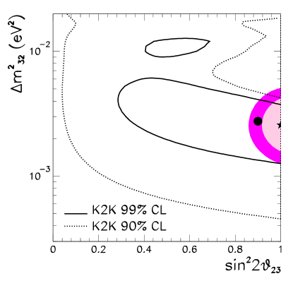
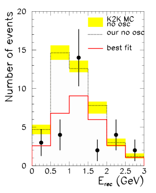
Figure 1: $\nu_{\mu}\rightarrow\nu_{\tau}$ oscillation analysis of K2K data. On the left panel we show the allowed (2d.o.f) regions on $\Delta m^{2},\sin^{2}2\theta$ at 90% CL (solid) and 99%CL (dotted). The best fit point is marked with a thick dot. The shadowed regions are the 90, and 99% CL of the atmospheric neutrino analysis with best point marked by a star. The right panel shows the spectrum of K2K events as a function of the reconstructed neutrino energy for the 6 bins used in the analysis. The data points are shown together with their statistical errors. The dotted histogram and the shadow boxes represent our prediction and the K2K MC prediction in the absence of oscillations respectively. The full line represents the expected distribution for the best fit point for $\nu_{\mu}\rightarrow\nu_{\tau}$ oscillations.

In the framework of 3$\nu$ mixing the analysis of K2K, atmospheric and CHOOZ data provides information on the parameters $\Delta m^{2}_{31}$, $\theta_{23}$, and $\theta_{13}$. We define:

$$\chi^{2}_{\rm ATM+CHOOZ+K2K}(\Delta m^{2}_{32},\theta_{23},\theta_{13})=\chi^{2}_{\rm ATM}(\Delta m^{2}_{32},\theta_{23},\theta_{13})$$

$$+\chi^{2}_{\rm CHOOZ}(\Delta m^{2}_{32},\theta_{13})+\chi^{2}_{\rm K2K}(\Delta m^{2}_{32},\theta_{23},\theta_{13})\;.$$ (8)

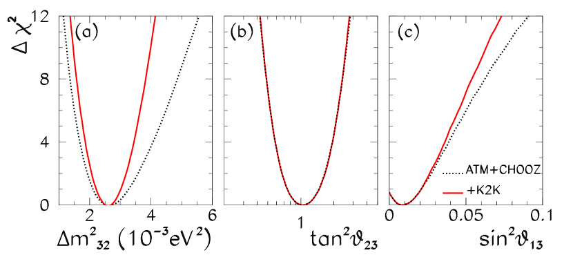
Figure 2: 3$\nu$ oscillation analysis of the atmospheric, CHOOZ and K2K data. The left, center and right panels show the dependence of $\Delta\chi^{2}$ on $\Delta m^{2}_{32}$, $\tan^{2}\theta_{23}$ and $\sin^{2}\theta_{13}$ for the analysis of atmospheric, CHOOZ and K2K data (full line) compared to the previous bound before the inclusion of K2K (dotted line). The individual 1  (3) $\sigma$ bounds in Eq. (9) can be read from the figure with the condition $\Delta\chi^{2}\leq 1\;(9)$.

In the three panels of Fig. 2 we show the bounds on each of the three parameters obtained from this analysis (full lines). For comparison we also show the corresponding ranges for the analysis of atmospheric and CHOOZ data alone (dotted lines). The corresponding subtracted minima are given in Table 1. The results in the figure are shown for the normal mass ordering, but once the constraint on $\theta_{13}$ from CHOOZ is included in the analysis, the differences between the results for normal and inverted mass ordering are minimal. The careful reader may notice that the $\chi^{2}$ per d.o.f. seems too good. As seen in Table 1 this effect is driven by the atmospheric data and it was already the case for the previous SK data sample. It is partly due to the very good agreement of the multi-GeV electron distributions with their no-oscillation expectations. However, as discussed in Ref. lisik2k , $\chi^{2}_{\rm min}$ is only 2$\sigma$ below its characteristic value, not low enough to be statistically suspected.

	ATMOS	ATMOS+CHOOZ	ATMOS+CHOOZ+K2K
Data points	65	65+14=79	65+14+6=85
$\frac{\Delta m^{2}_{32}}{\rm eV^{2}}$	$2.7\times 10^{-3}$	$2.55\times 10^{-3}$	$2.6\times 10^{-3}$
$\tan^{2}\theta_{23}$	1	1	1
$\sin^{2}\theta_{13}$	0.015	0.009	0.009
$\chi^{2}_{\rm min}$	39.7	45.8	55.1

Table 1: Minimum $\chi^{2}$ values and best-fit points for the $3\nu$ oscillation analysis of atmospheric, CHOOZ and K2K data.

In each panel the displayed $\chi^{2}$ has been marginalized with respect to the other two parameters. From the figure we see that the inclusion of K2K data in the analysis results into a reduction of the allowed range of $\Delta m^{2}_{32}$ while the allowed range of $\theta_{23}$ is not modified. The reduction is more significant for the upper bound of $\Delta m^{2}_{32}$ while the lower bound is slightly increased. More quantitatively we find that the following ranges of parameters are allowed at 1$\sigma$ (3$\sigma$) CL from this analysis

$$(1.5)\;2.2\;<\;\Delta m^{2}_{32}/10^{-3}\mbox{\rm eV${}^{2}$}\;<\;\;3.0\,(3.9)\;,$$

$$(0.45)\,0.75\;<\;\tan^{2}\theta_{23}\;<\;1.3\,(2.3)\;.$$ (9)

These ranges are consistent with the results from the 2-neutrino oscillation analysis of K2K and atmospheric data in Ref. lisik2k .

Concerning the “generic” 3$\nu$ mixing parameter $\theta_{13}$, Eq. (6) shows that its effect on both the normalization and the shape of the $\nu_{\mu}$ spectrum is further suppressed near maximal mixing by $\cos 2\theta_{23}\sim 0$. As a consequence K2K alone does not provide any bound on $\theta_{13}$. However Fig. 2.c illustrates how the inclusion of the long-baseline data results into a tightening of the bound on $\theta_{13}$ (at large CL) when combined with the atmospheric and CHOOZ data. This is an indirect effect due to the increase in the lower bound on $\Delta m^{2}_{32}$ . In the favoured range of $\Delta m^{2}_{32}$ the oscillating phase at CHOOZ is small enough so that it can be expanded and the oscillation probability of $\bar{\nu}_{e}$ depends quadratically on $\Delta m^{2}_{32}$. As a consequence the bound on the mixing angle from CHOOZ is a very sensitive function of the allowed values for $\Delta m^{2}_{32}$. The increase of the lower bound on $\Delta m^{2}_{32}$ due to the inclusion of the K2K data leads to the tightening of the derived limit on $\theta_{13}$ at high CL. From Fig. 2.c and Table 1 we also see that the best fit point is not exactly at $\sin^{2}\theta_{13}=0$, although this is not very statistically significant. This effect is due to the atmospheric neutrino data. In particular to the slight excess of sub GeV e-like events which is better described with a non-vanishing value of $\theta_{13}$.

III.2 Global Analysis

We calculate the global $\chi^{2}$ by fitting all the available data

$$\chi^{2}_{\rm global}(\Delta m^{2}_{21},\Delta m^{2}_{32},\theta_{12},\theta_{23},\theta_{13}) = \chi^{2}_{\rm solar}(\Delta m^{2}_{21},\theta_{12},\theta_{13})+\chi^{2}_{\rm Kland}(\Delta m^{2}_{21},\theta_{12},\theta_{13})$$ (10)

$$+\chi^{2}_{\rm atm}(\Delta m^{2}_{32},\theta_{23},\theta_{13})+\chi^{2}_{\rm K2K}(\Delta m^{2}_{32},\theta_{23},\theta_{13})$$

$$+\chi^{2}_{\rm CHOOZ}(\Delta m^{2}_{32},\theta_{13})\;.$$

The results of the global combined analysis are summarized in Fig. 3 and Fig. 4 in which we show different projections of the allowed 5-dimensional parameter space.

In Fig. 3 we plot the individual bounds on each of the five parameters derived from the global analysis (full line). To illustrate the impact of the K2K and KamLAND data we also show the corresponding bounds when K2K is not included in the analysis (dotted line) and when KamLAND is not included (dashed line). In each panel the displayed $\chi^{2}$ has been marginalized with respect to the other four parameters. The subtracted minima for each of the curves are given in Table 2.

Figure 3 illustrates that the dominant effects of including KamLAND are those derived in the two-neutrino oscillation analysis of solar and KamLAND data ourkland ; othersolkam : the determination of $\Delta m^{2}_{21}$ (panel a) to be in the LMA region and a very mild improvement of the allowed mixing angle $\theta_{12}$ (panel b). In other words, the inclusion of the 3$\nu$ mixing structure in the analysis of solar and KamLAND data does not affect the determination of these parameters once the additional angle $\theta_{13}$ is bounded to be small. The slight tightening of the $\theta_{13}$ limit due to the inclusion of K2K data does not have any impact in the determination of the bounds on $\Delta m^{2}_{21}$ and $\theta_{12}$. Quantitatively we find that the following ranges of parameters are allowed at 1$\sigma$ (3$\sigma$) CL from this analysis

$$(5.4)\;6.7\;<\;\Delta m^{2}_{21}/10^{-5}\mbox{\rm eV${}^{2}$}\;<\;\;7.7\,(10.)\;\;\;{\rm and}\;\;(14.)\;<\;\Delta m^{2}_{21}/10^{-5}\mbox{\rm eV${}^{2}$}\;<\;(19.)\;,$$

$$(0.29)\,0.39\;<\;\tan^{2}\theta_{12}\;<\;0.51\,(0.82)\;$$ (11)

The range of $\Delta m^{2}_{21}$ on the right of the first line in Eq. (11) correspond to solutions in the upper LMA island (see Fig. 4.a). At present the results of the solar and Kamland analysis still allow for this ambiguity in the determination of $\Delta m^{2}_{21}$ at CL $\gtrsim 2.5\sigma$. This reflects the departure from the parabolic (gaussian) behaviour of the $\Delta m^{2}_{21}$ dependence of $\chi_{\rm global}$ and the presence of a second local minima. With improved statistics KamLAND will be able to resolve this ambiguity othersolkam ; carlosnew .

Comparing the full line on the $\theta_{13}$ panel in Fig. 3.c with the corresponding one in Fig. 2.c we see that the inclusion of the solar+KamLAND data does have an impact on the allowed range of $\theta_{13}$. However the comparison of the full and dashed line in Fig. 3.c illustrates that the impact is due to the solar data. Eq. (5) shows that a small $\theta_{13}$ does not significantly affect the shape of the measured spectrum at KamLAND. On the other hand, the overall normalization is scaled by $\cos^{4}\theta_{13}$ and this factor has the potential to introduce a non-negligible effect (in particular in the determination of the mixing angle $\theta_{12}$  3kland ). Within its present accuracy, however, the KamLAND experiment cannot provide any further significant constraint on $\theta_{13}$. Altogether, the derived bounds on $\theta_{13}$ from the global analysis are:

$$\sin^{2}\theta_{13}<0.02\;(0.052)\;,$$ (12)

at 1$\sigma$ (3$\sigma$).

Finally, comparing Fig. 3.d and Fig. 3.e with the corresponding curves in Fig. 2.a and Fig. 2.b, we see that the additional restriction on the possible range of $\theta_{13}$ imposed by the solar data does not quantitatively affect the dominant effect of the inclusion K2K –the improved determination of $\Delta m^{2}_{32}$. Thus the allowed ranges of $\Delta m^{2}_{32}$ and $\theta_{23}$ in Eq. (9) are valid for the global analysis as well.

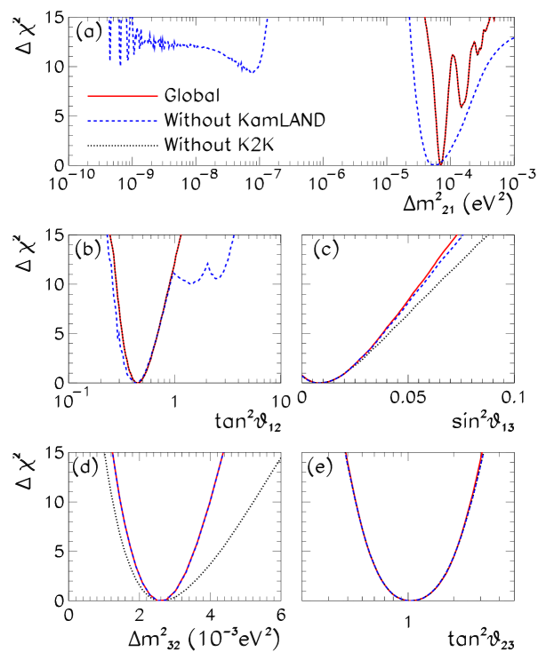
Figure 3: Global 3$\nu$ oscillation analysis. Each panels shows the dependence of $\Delta\chi^{2}$ on each of the five parameters from the global analysis (full line) compared to the bound prior to the inclusion of the K2K (dotted line) and KamLAND data (dashed line). The individual 1  (3) $\sigma$ bounds in Eqs. (11) and (12)  (9) can be read from the corresponding panel with the condition $\Delta\chi^{2}\leq 1\;(9)$.

The ranges in Eqs. (9), (11) and (12) are not independent. In Fig. 4 we plot the correlated bounds from the global analysis for each pair of parameters. The regions in each panel are obtained after marginalization of $\chi^{2}_{\rm global}$ in Eq (10) with respect to the three undisplayed parameters. The different contours correspond to regions defined at 90, 95, 99 % and 3$\sigma$ CL for 2d.o.f ($\Delta\chi^{2}=4.61,5.99,9.21,11.83$) respectively. From the figure we see that the stronger correlation appears between $\theta_{13}$ and $\Delta m^{2}_{32}$ as a reflection of the CHOOZ bound.

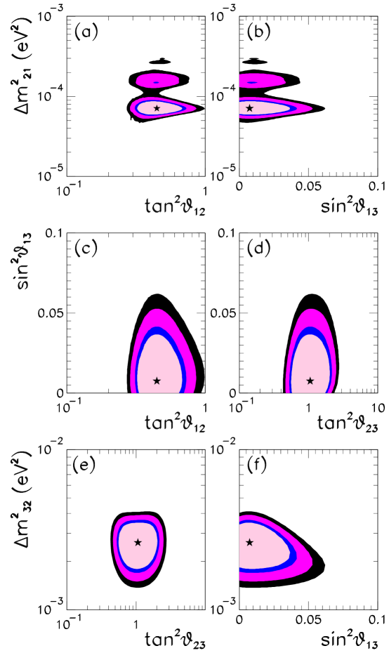
Figure 4: Global 3$\nu$ oscillation analysis. Each panels shows 2-dimensional projection of the allowed 5-dimensional region after marginalization with respect to the three undisplayed parameters. The different contours correspond to the two-dimensional allowed regions at 90, 95, 99 % and 3$\sigma$ CL.

	GLOBAL	GLOBAL-K2K	GLOBAL-KLAND
Data points	178	172	165
$\frac{\Delta m^{2}_{21}}{\rm eV^{2}}$	$7.1\times 10^{-5}$	$7.1\times 10^{-5}$	$5.8\times 10^{-5}$
$\tan^{2}\theta_{12}$	0.45	0.45	0.45
$\frac{\Delta m^{2}_{32}}{\rm eV^{2}}$	$2.6\times 10^{-3}$	$2.5\times 10^{-3}$	$2.6\times 10^{-3}$
$\tan^{2}\theta_{23}$	1	1	1
$\sin^{2}\theta_{13}$	0.009	0.009	0.009
$\chi^{2}_{\rm min}$	136	127	130

Table 2: Minimum $\chi^{2}$ values and best-fit points for the global $3\nu$ oscillation analysis.

In general, because of the correlations, the ranges in Eqs. (9), (11) and (12) cannot be directly used in deriving the corresponding entries in the $U$ mixing matrix as we discuss next.

III.3 Determination of the Leptonic Mixing Matrix

We describe in this section our procedure to consistently derive the allowed ranges for the magnitude of the entries of the leptonic mixing matrix. We start by defining the mass-marginalized $\chi^{2}$ function:

$$\chi^{2}_{\rm mix,global}(\theta_{12},\theta_{23},\theta_{13})={\rm min}_{(\Delta m^{2}_{21},\Delta m^{2}_{32})}\chi^{2}_{\rm global}(\Delta m^{2}_{21},\Delta m^{2}_{32},\theta_{12},\theta_{23},\theta_{13})\;.$$ (13)

We study the variation of $\chi^{2}_{\rm mix,global}$ as function of each of the mixing combinations in $U$ as follows. For a given magnitude $\overline{U_{ij}}$ of the entry $U(i,j)$ we define $\chi^{2}(\overline{U_{i,j}})$ as the minimum value of $\chi^{2}_{\rm mix,global}(\theta_{12},\theta_{23},\theta_{13})$ with the condition $|U(i,j)(\theta_{12},\theta_{23},\theta_{13})|=\overline{U_{i,j}}$. In this procedure the phase $\delta$ is allowed to vary freely between 0 and $\pi$. The allowed range of the magnitude of the entry $ij$ at a given CL is then defined as the values $\overline{U_{i,j}}$ verifying

$$\chi^{2}(\overline{U_{i,j}})-\chi^{2}_{\rm global,min}\leq\Delta\chi^{2}({\rm CL,1d.o.f})\;,$$ (14)

with $\chi^{2}_{\rm global,min}=136$. This is equivalent to having done the full analysis in terms of the independent matrix elements – of which, in the hierarchical approximation, only three are experimentally accessible at present (and can be chosen for instance to be $|U_{e2}|$, $|U_{e3}|$, and $|U_{\mu 3}|$)– and find the allowed magnitude of each $|U_{ij}|$ by marginalization of

$$\chi^{2}_{\rm mix,global}(|U_{e2}|,|U_{e3}|,|U_{\mu 3}|)\;,$$ (15)

with the use of unitarity relations and allowing a free relative phase $\delta$.

With this procedure we derive the following 90% (3$\sigma$) CL limits on the magnitude of the elements of the complete matrix

$$U=\begin{pmatrix}(0.73)\;0.79\;{\rm to}\;0.86\;(0.88)&(0.47)\;0.50\;{\rm to}\;0.61\;(0.67)&0\;{\rm to}\;0.16\;(0.23)\cr(0.17)\;0.24\;{\rm to}\;0.52\;(0.57)&(0.37)\;0.44\;{\rm to}\;0.69\;(0.73)&(0.56)\;0.63\;{\rm to}\;0.79\;(0.84)\cr(0.20)\;0.26\;{\rm to}\;0.52\;(0.58)&(0.40)\;0.47\;{\rm to}\;0.71\;(0.75)&(0.54)\;0.60\;{\rm to}\;0.77\;(0.82)\end{pmatrix}\;.$$ (16)

By construction the derived limits in Eq. (16) are obtained under the assumption of the matrix $U$ being unitary. In other words, the ranges in the different entries of the matrix are correlated due to the fact that, in general, the result of a given experiment restricts a combination of several entries of the matrix, as well as to the constraints imposed by unitarity. As a consequence choosing a specific value for one element further restricts the range of the others.

III.4 $\Delta m^{2}_{21}$ oscillations at future LBL experiments

In general, correlations between the allowed ranges of the parameters have to be considered when deriving the present bounds for any quantity involving two of more parameters. This is the case, for example, when predicting the allowed range of CP violation at future experiments as discussed in Ref. lisi3sol .

Here we explore the possible size of effects associated with $\Delta m^{2}_{21}$ oscillations (both CP violating and CP conserving) at future LBL experiments to be performed either with conventional superbeams SB (conventional meaning from the decay of pions generated from a proton beam dump) at a Neutrino Factory NF with neutrino beams from muon decay in muon storage rings .

The “golden” channel at these facilities involve the observation of either “wrong-sign” muons due to $\nu_{e}\rightarrow\nu_{\mu}$ (or $\bar{\nu}_{e}\rightarrow\bar{\nu}_{\mu}$) oscillations at a neutrino factory or or the detection of electrons (positrons) due to $\nu_{\mu}\rightarrow\nu_{e}$ ($\bar{\nu}_{\mu}\rightarrow\bar{\nu}_{e}$) at conventional superbeams . In either case the relevant oscillation probabilities in vacuum are accurately given by golden ; otherCP

$$P_{\nu_{e}\nu_{\mu}} = s_{23}^{2}\sin^{2}2\theta_{13}\sin^{2}\left(\frac{\Delta m^{2}_{32}L}{4E}\right)+c_{23}^{2}\sin^{2}2\theta_{12}\left(\frac{\Delta m^{2}_{21}L}{4E}\right)^{2}$$ (17)

$$+\tilde{J}\cos\left(\delta+\frac{\Delta m^{2}_{32}L}{4E}\right)\left(\frac{\Delta m^{2}_{21}L}{4E}\right)\sin\left(\frac{\Delta m^{2}_{32}L}{4E}\right)=P^{\rm atm}+P^{\rm sol}+P^{\rm inter}\;,$$

with $\tilde{J}=c_{13}\sin 2\theta_{12}\sin 2\theta_{13}\sin 2\theta_{23}$. $P^{\rm sol}$ contains the contribution to the probability due to longer wavelength oscillations while $P^{\rm inter}$ gives the interference between the longer and shorter wavelength oscillations and contains the information on the CP-violating phase $\delta$. In order to quantify the present bounds on these contributions we factorize the baseline and energy independent parts as:

$$P^{\rm sol}=(F^{\rm sol})^{2}\left(\frac{L}{4E}\right)^{2} P^{\rm inter}=F^{\rm inter}\cos\left(\delta-\frac{\Delta m^{2}_{32}L}{4E}\right)\sin\left(\frac{\Delta m^{2}_{32}L}{4E}\right)\left(\frac{L}{4E}\right)\;,$$

$$F^{\rm sol}=c_{23}\sin 2\theta_{12}\Delta m^{2}_{21} F^{\rm inter}=c_{13}\sin 2\theta_{12}\sin 2\theta_{13}\sin 2\theta_{23}\Delta m^{2}_{21}\;.$$ (18)

For very long baselines, for which the presence of matter cannot be neglected, the expressions above for $F^{\rm sol}$ and $F^{\rm inter}$ still hold as the coefficients of the dominant contributions to the probabilities in the expansion in the small parameters $\theta_{13}$ and $\Delta m^{2}_{21}$ golden ; otherCP .

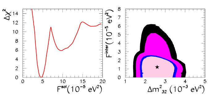
Figure 5: (a) Dependence of $\Delta\chi^{2}$ on $F^{\rm sol}$. (b) Allowed regions of $F^{\rm inter}$ versus $\Delta m^{2}_{32}$ at 90, 95, 99% and 3$\sigma$. The best value is marked with a star.

We show in Fig. 5 the present bounds on the coefficients $F^{\rm sol}$ and $F^{\rm inter}$. In general the dependence on $\Delta m^{2}_{32}$ of the interference term cannot be factorized because, depending on the considered baseline and energy, the oscillating phase with $\Delta m^{2}_{32}$ may be not small enough to be expanded. For this reason we show in Fig. 5.b the 2-dimensional allowed region of $F^{inter}$ versus $\Delta m^{2}_{32}$. In the figure we mark with a star the best value for $F^{inter}$ as obtained from this analysis which is not vanishing due to the small but non-zero best fit value of $\sin\theta_{13}$. This is, however, not statistically significant as $F^{inter}=0$ is at $\Delta\chi^{2}=0.9$. The negative slope in the upper part of the 90% and 95% CL region in Fig. 5.b is a reflection of the anti-correlation between the $\Delta m^{2}_{32}$ and $\sin^{2}\theta_{13}$ constraints from the CHOOZ experiment (see Fig. 4.f)

From this study we find the following 1$\sigma$ (3$\sigma)$ [1d.o.f] bounds

$$F^{\rm sol}/(10^{-5}{\rm eV}^{2}) =4.6\pm 0.6\;(4.6^{+2.1}_{-1.6}\;\;{\rm and}\;9.5^{+3.5}_{-2.0})\;,$$ (19)

$$0< F^{\rm inter}/(10^{-5}{\rm eV}^{2}) <1.9\;(5.5)\;,$$ (20)

where the bounds on $F^{\rm inter}$ are shown for the best fit value of $\Delta m^{2}_{32}=0.0026$ eV². The larger values for the 3$\sigma$ range in Eq.(19) and $F^{\rm inter}$ correspond to solutions of the solar+KamLAND analysis lying in the higher $\Delta m^{2}_{21}$ island (see Fig. 4.a and discussion below Eq. (11)).

IV Summary and Conclusions

We have presented the results of an updated global analysis of solar, atmospheric, reactor and long-baseline neutrino data in the context of three-neutrino oscillations making special emphasis on the impact of the recent long baseline $\nu_{\mu}$ disappearance data from the K2K experiment and reactor $\bar{\nu}_{e}$ disappearance from the KamLAND experiment. We find that the dominant effect of the inclusion of K2K and KamLAND data is the reduction of the allowed range of $\Delta m^{2}_{32}$ and $\Delta m^{2}_{21}$ respectively while the impact on the mixing angles $\theta_{23}$ and $\theta_{12}$ is marginal. The increase of the lower bound on $\Delta m^{2}_{32}$ due to the inclusion of the K2K data leads also to a slight tightening of the derived limit on $\theta_{13}$ at high CL. Our results on the individual allowed ranges for the oscillation parameters are given in Eqs. (9), (11) and (12) and graphically displayed in Fig. 3. The correlations between the derived bounds are illustrated i in Fig. 4. As outcome of the analysis we have presented in Eq. (16) our up-to-date best determination of the magnitude of the elements of the complete leptonic mixing matrix. Finally we have quantified the allowed contribution of $\Delta m^{2}_{21}$ oscillations to CP-odd and CP-even observables at future long baseline experiments with results presented in Fig. 5 and Eqs. (19) and (20).

APPENDIX A: ANALYSIS OF K2K DATA

In this appendix we describe our calculation of the K2K spectrum and our statistical analysis of the K2K data k2kprl .

We use in our statistical analysis the K2K data on the spectrum of single-ring $\mu$-like events. K2K present their results as the number of observed events as a function of the reconstructed neutrino energy. The reconstructed neutrino energy is determined from the observed $\mu$ energy in the event, $E_{\mu}$, and its scattering angle with respect to the incoming beam direction, $\cos\theta_{\mu}$, as

$$E_{\rm rec}=\frac{m_{N}E_{\mu}-\frac{m_{\mu}^{2}}{2}}{m_{N}-E_{\mu}+p_{\mu}\cos\theta_{\mu}}\;,$$ (21)

where $m_{N}$ is the nucleon mass. In Fig. 1 we show their data binned in five 0.5GeV bins with $0<E_{\rm rec}<2.5$ plus one bin containing all events above $2.5$ GeV. The total sample corresponds to 29 events. In the absence of oscillations 44 events were expected.

For QE events, $\nu_{\mu}\,n\rightarrow\mu\,p$ , and assuming perfect $E_{\mu}$ and $\cos\theta_{\mu}$ determination, $E_{\rm rec}=E_{\nu}$. Experimental energy and angular resolution, nuclear effects, and, more importantly, the contamination from non-QE (nQE) events, $\nu_{\mu}N\rightarrow\mu X$, in the sample, result into important deviations of the defined $E_{\rm rec}$ from the real $E_{\nu}$. From simple kinematics one finds that in nQE events there is a shift in the reconstructed neutrino energy with respect to the true neutrino energy

$$E_{\rm rec}=E_{\nu}\left[1+\frac{M_{X}^{2}-m_{N}^{2}}{m_{N}E_{\mu}-\frac{m_{\mu}^{2}}{2}}\right]^{-1}<E_{\nu}\;,$$ (22)

where $M_{X}$ is the invariant mass of the hadronic system produced together with the muon in the $\nu_{\mu}$ interaction. At the K2K energies the most important nQE contamination comes from single pion production. which occurs via the $\Delta$ resonance. At the largest energies there is a small contribution from deep inelastic scattering.

Thus in general the observed spectrum of single-ring $\mu$-like events in K2K can be obtained as kobayashi

$$N^{\rm th}(E_{\rm rec}) = N_{\rm norm}\int\Phi_{SK}(E_{\nu})\,P_{\mu\mu}(E_{\nu})\big{[}\sigma_{QE}(E_{\nu})\,\epsilon_{QE}^{1R_{\mu}}(E_{\nu})\,r_{QE}(E_{\nu},E_{\rm rec})+$$ (23)

$$f_{nQE}\,\sigma_{nQE}(E_{\nu})\,\epsilon_{nQE}^{1R_{\mu}}(E_{\nu})\,r_{nQE}(E_{\nu},E_{\rm rec})\big{]}dE_{\nu}\;,$$

where $\Phi_{SK}(E_{\nu})$ is the expected $\nu_{\mu}$ spectrum at the SK site in the absence of oscillations. $P_{\mu\mu}(E_{\nu})$ is the survival probability of $\nu_{\mu}$ for a given set of oscillation parameters. $f_{nQE}=0.93$ is a rescale factor of the expected contamination from nQE events as obtained from MC simulation by the K2K collaboration k2kprl . $\sigma_{QE(nQE)}(E_{\nu})$ are the neutrino interaction cross sections. $\epsilon_{QE(nQE)}^{1R_{\mu}}$ are the detection efficiencies for 1-ring $\mu$-like events at SK. $r_{QE(nQE)}(E_{\nu},E_{\rm rec})$ are the functions relating the reconstructed energy and the true neutrino energy. $N_{\rm norm}$ is the normalization factor which is chosen so that in the absence of oscillations the total integral gives 44 events.

In our calculation we use the neutrino spectrum $\Phi_{SK}$ as provided by the K2K collaboration kobayashi ; kobaprivate . This flux was estimated from the flux measured in the near detector by multiplying it by a MC simulated ratio of the fluxes between the near and far detectors. We further assume that the detection efficiencies for 1-ring $\mu$-like events at SK are the same for the K2K analysis as for the atmospheric neutrino analysis (further details and references can be found in Ref. ouratmos ).

At present there is not enough information from the K2K collaboration on the $r_{QE(nQE)}(E_{\nu},E_{\rm rec})$ functions. In our calculation we have used a physically-motivated form for those functions. We include in the functions $r_{QE(nQE)}(E_{\nu},E_{\rm rec})$ the dominant effect in the missreconstruction of the neutrino energy: the shift in the reconstructed neutrino energy due to the different kinematics of the nQE events as described by Eq. (22). We also include the (subdominant) effects due to the experimental energy and angular resolutions which smear the measured muon energy $E_{\mu}$ and angle $\theta_{\mu}$ around their true values $E^{\prime}_{\mu}$ and $\theta^{\prime}_{\mu}$:

$$r_{QE}(E_{\nu},E_{\rm rec})=\frac{1}{\sigma_{QE}(E_{\nu})} \int dE^{\prime}_{\mu}dE_{\mu}d\theta\frac{d\sigma_{QE}(E_{\nu},E^{\prime}_{\mu})}{dE^{\prime}_{\mu}}{\rm Res_{E}}(E_{\mu}-E_{\mu}^{\prime}){\rm Res_{\theta}}(\theta_{\mu}-\theta_{\mu}^{\prime})\delta(E_{\nu}-E^{\prime}_{\rm rec})$$

$$r_{nQE}(E_{\nu},E_{\rm rec})=\frac{1}{\sigma_{nQE}(E_{\nu})} \int dE^{\prime}_{\mu}dE_{\mu}d\theta dM_{X}\frac{d\sigma_{nQE}(E_{\nu},E^{\prime}_{\mu},M_{X})}{dE^{\prime}_{\mu}dM_{X}}{\rm Res_{E}}(E_{\mu}-E_{\mu}^{\prime}){\rm Res_{\theta}}(\theta_{\mu}-\theta_{\mu}^{\prime})$$ (24)

$$\delta\left(E_{\nu}-E^{\prime}_{\rm rec}\left[1+\frac{M_{X}^{2}-m_{N}^{2}}{m_{N}E^{\prime}_{\mu}-\frac{m_{\mu}^{2}}{2}}\right]^{-1}\right)$$

where

$$E^{\prime}_{\rm rec}=E_{\rm rec}\frac{m_{N}E_{\mu}-\frac{m_{\mu}^{2}}{2}}{m_{N}-E_{\mu}+p_{\mu}\cos\theta^{\prime}_{\mu}}\frac{m_{N}-E^{\prime}_{\mu}+p^{\prime}_{\mu}\cos\theta_{\mu}}{m_{N}E^{\prime}_{\mu}-\frac{m_{\mu}^{2}}{2}}\;,$$

$${\rm Res_{E}}(E^{\prime}_{\nu}-E_{\nu})=\frac{1}{\sqrt{2\pi}\sigma_{E}}{\mbox{\Large e}}^{-\frac{1}{2}\frac{(E_{\mu}-E_{\mu}^{\prime})^{2}}{\sigma_{E}^{2}}}\;,$$

$${\rm Res_{\theta}}(\theta^{\prime}_{\nu}-\theta_{\nu})=\frac{1}{\sqrt{2\pi}\sigma_{\theta}}{\mbox{\Large e}}^{-\frac{1}{2}\frac{(\theta_{\mu}-\theta_{\mu}^{\prime})^{2}}{\sigma_{\theta}^{2}}}\;.$$ (25)

Following SK data skatmpub we use an energy resolution for the muons of $\sigma_{E}/E_{\mu}=3$% and an angular resolution $\sigma_{\theta}=3^{\circ}$ (see also Ref. campanelli for further details). Notice that in the expressions above the true angle of the muon, $\theta_{\mu}^{\prime}$, is not an independent variable but it is related by the kinematics of the process to the initial neutrino energy, $E_{\nu}$, the final muon energy, $E_{\mu}^{\prime}$, and the invariant mass of the hadronic system, $M_{X}$. The final result on the number of expected events in each $E_{\rm res}$ bin is obtained by substituting Eqs. (24) and (25) in Eq. (23) and numerically integrating for the kinematical variables in the corresponding range of $E_{\rm res}$. In this procedure the only free parameter to adjust is the overall normalization. The shape of the spectrum is then fully determined.

In order to verify the quality of our simulation we compare our predictions for the energy distribution of the events with the Monte Carlo simulations of the K2K collaboration in absence of oscillation. In Fig. 1 we show our predictions superimposed with those from the experimental Monte Carlo (obtained from Fig.2 in Ref. k2kprl ), both normalized to the 44 expected events in the absence of oscillations. The boxes for the MC prediction represent the systematic error bands. We can see that the agreement in the shape of the spectrum is very good.

In our statistical analysis of the K2K data we use Poisson statistics as required given the small number of events. We include the systematic uncertainties associated with the determination of the neutrino energy spectrum in the near detector (ND), the model dependence of the amount of nQE contamination parameter $f_{nQE}$, the near/far extrapolation (F/N) and the overall flux normalization (NOR) kobayashi ; kobaprivate . The errors on the first three items depend on energy and have correlations among the different energy bins. We account for all these effects by using the $\chi^{2}$ function kobayashi ; lisik2k ; kobaprivate :

$$\chi^{2}_{K2K}={\rm min}_{f} \Big{[} 2\sum_{i=1}^{6}\left(\bar{N}_{i}^{\rm th}-N_{i}^{\rm exp}-N_{i}^{\rm exp}\ln\frac{\bar{N}_{i}^{\rm th}}{N_{i}^{\rm exp}}\right)+\sum_{j,k=1}^{6}f^{F/N}_{j}(\rho^{F/N})^{-1}_{ij}f^{F/N}_{j}$$ (26)

$$+\sum_{j,k=1}^{7}f^{ND,nQE}_{j}(\rho^{ND,nQE})^{-1}_{ij}f^{ND,nQE}_{j}+{f^{NOR}}^{2}\Big{]}\;,$$

where $\bar{N}_{i}^{\rm th}=N_{i}^{\rm th}(1+f^{F/N}_{i}\sigma^{F/N}_{i}+f^{ND}_{i}\sigma^{ND}_{i}+f^{nQE}\sigma^{nQE}_{i}+f^{NOR}\sigma^{NOR})$. By ${\rm min}_{f}$ we denote the minimization with respect to the systematic shift parameters (or pulls lisik2k ) $f^{F/N}_{i=1,6}$, $f^{ND}_{i=1,6}$, $f^{nQE}$, and $f^{NOR}$ We use the systematic errors and their correlations as provided by K2K collaboration k2kprl ; kobayashi ; kobaprivate . For instance

$$\sigma^{NOR} = 5\%\;,$$

$$\sigma^{F/N}_{i} = 2.5\%\;,\;4.3\%\;,\;6.5\%\;,\;10.4\%\,\;11.1\%\;,12.2\%\;,$$

$$\sigma^{ND}_{i} = 49\%\;,\;7.1\%\;,\;0\%\;,\;7.1\%\,\;8.4\%\;,11.1\%\;,$$ (27)

$$\sigma^{nQE}_{i} = 13\%\;,\;8.9\%\;,\;6\%\;,\;3.8\%\,\;3.\%\;,5.5$$

for $i=1,6$ respectively.

Thus in our analysis we use both the shape and the normalization of the 29 single-ring $\mu$-like events. In their analysis K2K uses only the spectrum shape (but not the normalization) of the 29 single-ring $\mu$-like events plus the overall normalization of their total sample of fully contained events (a total of 56). We cannot use the normalization from the additional 27 events in the lack of more detailed information from the K2K collaboration on the efficiencies for multi-ring events. Nevertheless, as described in Sec. III.1, the results of our oscillation analysis are in good agreement with those from the K2K analysis.

- (1) M.Shiozawa, SuperKamiokande Coll., in XXth International Conference on Neutrino Physics and Astrophysics, Munich May 2002, (http://neutrino2002.ph.tum.de).
- (2) Y. Fukuda et al., Phys. Lett. B433, (1998) 9; Phys. Lett. B436, (1998) 33 ; Phys. Lett. B467, (1999) 185 ; Phys. Rev. Lett. 82, (1999) 2644.
- (3) M.Ambrosio et al., MACRO Coll., Phys. Lett. B 517, (2001) 59. M. Goodman, XXth International Conference on Neutrino Physics and Astrophysics, Munich May 2002. (http://neutrino2002.ph.tum.de).
- (4) D. A. Petyt [SOUDAN-2 Collaboration], Nucl. Phys. Proc. Suppl. 110, 349 (2002).
- (5) Q. R. Ahmad et al., Phys. Rev. Lett. 87, 071301 (2001); Q. R. Ahmad et al., ibid. 89 011301 (2002)
- (6) S. Fukuda et al. [Super-Kamiokande Collaboration], Phys. Lett. B 539, 179 (2002)
- (7) B. T. Cleveland et al., Astrophys. J. 496, 505 (1998).
- (8) J. N. Abdurashitov et al., J. Exp. Theor. Phys. 95, 181 (2002).
- (9) GALLEX collaboration, W. Hampel et al., Phys. Lett. B 447, 127 (1999).
- (10) T. Kirsten, talk at the XXth International Conference on Neutrino Physics and Astrophysics (NU2002), Munich, (May 25-30, 2002); M. Altmann et al., Phys. Lett. B 490, 16 (2000); GNO collaboration, E. Bellotti et al., in Neutrino 2000, Proc. of the XIXth International Conference on Neutrino Physics and Astrophysics, 16–21 June 2000, eds. J. Law, R. W. Ollerhead, and J. J. Simpson, Nuclear Phys. B (Proc. Suppl.) 91, 44 (2001).
- (11) Y. Fukuda et al., Phys. Rev. Lett. 77, 1683 (1996).
- (12) J. N. Bahcall, N. A. Bahcall and G. Shaviv, Phys. Rev. Lett. 20, (1968) 1209 ; J. N. Bahcall and R. Davis, Science 191, (1976)264.
- (13) M. H. Ahn et al., Phys. Rev. Lett. 90, 041801 (2003)
- (14) K. Eguchi et al. [KamLAND Collaboration], Phys. Rev. Lett. 90, 021802 (2003)
- (15) J. N. Bahcall, M. C. Gonzalez-Garcia and C. Pena-Garay, JHEP 0207, 054 (2002)
- (16) J. N. Bahcall, M. C. Gonzalez-Garcia and C. Pena-Garay, JHEP 0302, 009 (2003)
- (17) G. L. Fogli, E. Lisi, A. Marrone, D. Montanino, A. Palazzo and A. M. Rotunno, Phys. Rev. D 67, 073002 (2003); M. Maltoni, T. Schwetz and J.W. Valle, hep-ph/0212129; P. Creminelli, G. Signorelli and A. Strumia, J. High Energy Phys. 05 (2001) 052 [hep-ph/0102234]; A. Bandyopadhyay, S. Choubey, R. Gandhi, S. Goswami and D.P. Roy, Phys. Lett.B 559 (2003) 121; P.C. de Holanda and A.Y. Smirnov, J. Cosmol. Astropart. Phys. 02 (2003) 001; H. Nunokawa, W.J. Teves and R. Zukanovich Funchal, Phys. Lett. B 562, 28 (2003); A.B. Balantekin and H. Yuksel, J. Phys. G 29, 665 (2003) V. Barger and D. Marfatia, Phys. Lett. B 555 (2003) 144; P. Aliani, V. Antonelli, M. Picariello and E. Torrente-Lujan, hep-ph/0212212.
- (18) For a recent review see M.C. Gonzalez-Garcia and Y. Nir, Rev. Mod. Phys. 75 345 (2003).
- (19) B. Pontecorvo, J. Exptl. Theoret. Phys. 33, 549 (1957) [Sov. Phys. JETP 6, 429 (1958)]; Z. Maki, M. Nakagawa and S. Sakata, Prog. Theo. Phys. 28, (1962) 870 ; M. Kobayashi and T. Maskawa, Prog. Theor. Phys. 49, (1973) 652;
- (20) Particle Data Group, D. E. Groom et al., Eur. Phys. J.C15, (2000) 1.
- (21) S. M. Bilenky, J. Hosek and S. T. Petcov, Phys. Lett. B 94, 495 (1980).
- (22) M. Apollonio et al., Phys. Lett. B 466, 415 (1999).
- (23) N. Fornengo, M. C. Gonzalez-Garcia and J. W. Valle, Nucl. Phys. B 580, 58 (2000); M. C. Gonzalez-Garcia, H. Nunokawa, O. L. Peres and J. W. Valle, Nucl. Phys. B 543, 3 (1999); M. C. Gonzalez-Garcia, H. Nunokawa, O. L. Peres, T. Stanev and J. W. Valle, Phys. Rev. D 58, 033004 (1998).
- (24) M. C. Gonzalez-Garcia, M. Maltoni, C. Pena-Garay and J. W. Valle, Phys. Rev. D 63, 033005 (2001)
- (25) M. C. Gonzalez-Garcia and M. Maltoni, Eur. Phys. J. C 26, 417 (2003)
- (26) J. N. Bahcall, M. H. Pinsonneault, and S. Basu, Astrophys. J. 555, 990 (2001).
- (27) R. Foot, R.R. Volkas and O. Yasuda, Phys. Rev. D58, (1998) 013006; O. Yasuda, Phys. Rev. D58, (1998) 091301; E.Kh. Akhmedov, A. Dighe, P. Lipari and A.Yu. Smirnov, Nucl. Phys. B542, (1999) 3;
- (28) E. Lisi and D. Montanino, Phys. Rev. D56, (1997) 1792.
- (29) A.M. Dziewonski and D.L. Anderson, Phys. Earth Planet. Inter. 25, (1981) 297.
- (30) S. M. Bilenky, D. Nicolo and S. T. Petcov, Phys. Lett. B 538, 77 (2002); S. T. Petcov and M. Piai, Phys. Lett. B 533, 94 (2002).
- (31) I. Mocioiu and R. Shrock, JHEP 0111, (2001) 050.
- (32) G. L. Fogli, E. Lisi, A. Marrone and D. Montanino, hep-ph/0303064.
- (33) J. N. Bahcall and C. Pena-Garay, hep-ph/0305159.
- (34) M. C. Gonzalez-Garcia and C. Peña-Garay, Phys. Lett. B 527, 199 (2002).
- (35) G. L. Fogli,G. Lettera, E. Lisi, A. Marrone, A Palazzo, and A. Rotunno, Phys. Rev. D66 093008 (2002).
- (36) B. Richter, hep-ph/0008222; V. D. Barger, S. Geer, R. Raja and K. Whisnant, Phys. Rev. D 63, 113011 (2001); J. J. Gomez-Cadenas et al., hep-ph/0105297; Y. Itow, et al., hep-ex/0106019; M. V. Diwan et al., hep-ph/0303081.
- (37) S. Geer, Phys. ReV. D57 6989 (1998). A. De Rujula, M. B. Gavela and P. Hernandez, Nucl. Phys. B 547, 21 (1999); J. J. Gomez-Cadenas and D. A. Harris, FERMILAB-PUB-02-044-T.
- (38) A. Cervera, A. Donini, M. B. Gavela, J. J. Gomez Cadenas, P. Hernandez, O. Mena and S. Rigolin, Nucl. Phys. B 579, 17 (2000).
- (39) H.W. Aagluer,K.H.Shwarzer, Z.Phys. C40 (1988) 273; M. Freund, Phys. Rev. D 64, 053003 (2001); K.Kimura, A. Takamura, and H. Yokomakura, Phys. Rev. D 66, 073005 (2002).
- (40) T. Kobayashi, Proceedings of the 4th International Workshop on Neutrino Factories based on Muon Storage Rings, (London, July 2002) http://www.hep.ph.ic.ac.uk/NuFact02 .
- (41) Private communication with K2K collaboration
- (42) A. Blondel, M. Campanelli, and M. Fechner, Proceedings of the 4th International Workshop on Neutrino Factories based on Muon Storage Rings (London, July 2002) http://www.hep.ph.ic.ac.uk/NuFact02 .