BROWN-HET-1360; CU-TP-1089; MIT-CTP-3389

June 2003

hep-lat/0306038

A Review Of Two Novel Numerical Methods in QFT

R. Easther¹, D. D. Ferrante², G. S. Guralnik^3, and D. Petrov²

¹ Department of Physics

Columbia University, NY — 10027, NY.

²Department of Physics

Brown University, Providence — 02912, RI.

³Center for Theoretical Physics

Massachusetts Institute of Technology, Cambridge — 02139, MA.

We outline two alternative schemes to perform numerical calculations in quantum field theory. In principle, both of these approaches are better suited to study phase structure than conventional Monte Carlo. The first method, Source Galerkin, is based on a numerical analysis of the Schwinger-Dyson equations using modern computer techniques. The nature of this approach makes dealing with fermions relatively straightforward, particularly since we can work on the continuum. Its ultimate success in non-trivial dimensions will depend on the power of a propagator expansion scheme which also greatly simplifies numerical calculation of traditional perturbation graphs. The second method extends Monte Carlo approaches by introducing a procedure to deal with rapidly oscillating integrals.

1 Introduction

Over the last two decades, Monte Carlo numerical methods applied to lattice quantum field theory have allowed us to perform many important calculations, and have verified and extended our basic understanding of elementary particle phenomena. While very informative, these calculations still do not fully reflect the potential of these methods because it has been impossible to obtain the multiple teraflop-years of computer time required for very accurate non-quenched fermionic calculations. The promise of “definitive” lattice QCD calculations has helped to drive the development of supercomputers to the point where computer clusters are beginning to sustain speeds of several teraflops. Over the next few years, many teraflop-years will be devoted to lattice QCD, and it is likely that the range and accuracy of prediction of QFT using numerical calculation will be greatly extended.

However, even with this promise of great resources, numerical field theory calculations are far from becoming mechanical. While large blocks of computing time on fast new machines should make it possible to deal with the fermion determinant, the effort of doing so and dealing with lattice artifacts guarantee that it will still be difficult to extract reasonable numerical information about fermionic systems. Moreover, calculations involving non-positive definite actions, actions with rapid oscillations, phase transitions and symmetry breaking are generally resistant or intractable to solution by Monte Carlo methods. Many problems, such as general scattering, are just too computationally intensive to be accessible. Motivated by these issues, we are in the process of developing two supplementary approaches to traditional numerical quantum field theory. The first is the “Source Galerkin Method” (SG)[2, 3, 4] which uses nested approximations to the Schwinger–Dyson equations. The second is a tuned Monte Carlo method, “Mollified Monte Carlo” (MMC)[8, 10, 4] which uses an averaging process to smooth regions of high oscillation in path integrals. Conceptually distinct, these methods actually have similar starting points. MMC uses information from stationary phase points of an action, while SG methods are easiest to implement if they are iteratively constructed around stationary phase points.

2 Source-Galerkin Methods

The Monte Carlo approach suffers from at least two serious intrinsic problems associated with fermions. The first is that, in order to apply this technique, it is essential to formulate a field theory on a space time lattice rather than on the continuum. Any calculation, of necessity, involves an extrapolation to the continuum for the final result. As a consequence of the lattice, it is necessary to introduce extra degrees of freedoms for fermionic fields. This produces artifacts which are difficult to control. The second problem arises from the fact that we can not directly perform Monte Carlo sampling on integrals with the anti-commuting Grassman variables requisite for fermions. Consequently, any fermionic degrees of freedom must be explicitly removed by partial integration of the lattice path integral. These integrations result in the very non-local “fermion determinant” which requires multi-teraflop computer power to evaluate to high accuracy.

We introduced the Source Galerkin method to deal with these two fermionic problems and the difficulties associated with phase structure mentioned in the introduction. The SG method is based on an iterative set of approximations to the Schwinger-Dyson equations. It is defined on the continuum and has the nice property that fermions (except for anti-commutativity) are treated in the same way as bosons. Most of the basic concepts of the SG method can be demonstrated by its application to single field models. In particular, we can get some understanding of why it is possible to deal with phase structure issues. Therefore, in the interest of simplicity, we avoid directly addressing the details of fermionic calculations here and confine this discussion to these models. The basic ideas of how fermions work can easily be extrapolated from a primitive lattice precursor of this model [5].

We start with the simple assumption that the Quantum Field Theory (QFT) action is written with sources $J_{i}(x)$ for every field $\phi_{i}(x)$ so that the vacuum functional $Z=\langle+0|0-\rangle_{J_{i}}$ satisfies the differential equation,

$$\underbrace{F\Bigl{(}\frac{\delta}{\delta J_{i}(x)}\Bigr{)}}_{\begin{subarray}{c}\text{essentially the}\\ \text{field equations}\end{subarray}}\,\mathcal{Z}=0\;.$$

A familiar but far from straightforward example of this is $\phi^{4}$ scalar QFT

$$(\partial^{2}+m^{2})\,\phi(x)+g\,\phi^{3}(x)=J(x)\;$$

which, in Euclidean space, gives the very non-trivial set of coupled differential equations:

$$\Biggl{[}(\partial^{2}_{x}+m^{2})\,\frac{\delta}{\delta J(x)}+g\,\Bigl{(}\frac{\delta}{\delta J(x)}\Bigr{)}^{3}-J(x)\Biggr{]}\mathcal{Z}[J]=0\;.$$

2.1 The Ultra-Local $\boldsymbol{\phi}^{\mathbf{4}}$

Figure 1: Path integrals must start and end at $\infty$ in hatched regions.

To further simplify, we examine the above quartic field theory in zero dimensions. We will show that even this case has a rich basic structure which is not directly accessible by normal Monte Carlo approaches. Our demonstration example then reduces to the linear differential equation

$$\Biggl{[}m^{2}\,\frac{d}{dJ}+g\,\Bigl{(}\frac{d}{dJ}\Bigr{)}^{3}-J\Biggr{]}\mathcal{Z}[J]=0\;.$$ (1)

Since this has three independent solutions, three independent parameters are required to specify the full solution [1]. If we rewrite $Z[J]$ as a power series,

$$Z[J]=Z[0]\,\sum_{k=0}^{\infty}\,\frac{1}{k!}\,G_{k}\,J^{k}\;;$$

equation (1) leads to the recursion relations:

$$g\,G_{n+3}+m^{2}\,G_{n+1}-n\,G_{n-1}=0\;.$$

These have three independent solutions that can be expressed in terms of parabolic cylinder functions.[1] This is a useful test system, since it is computationally non-trivial, but has solutions in terms of well known functions, making it is easy to check the validity of a new numerical approximation technique. Note that, with the proper choice of parameters, solutions exist with non-vanishing odd Green’s functions.

Figure 2: Three convenient independent paths.

It is usual to think of the path integral formulation of QFT as being defined by a process involving evaluation of integrals along the entire real axis. However, this cannot yield a complete description of the ultra local quartic theory, since it is impossible to generate non-zero odd-order Green’s functions from actions with only even powers of fields, when path integrals are only evaluated in this way. As a generalization of this, we see that a choice of path confined to the real axis removes the possibility of spontaneous symmetry breaking! Very specifically, it is straightforward to show that the one dimensional path integral along the whole real axis for the above zero dimensional field theory does not produce the full solution set outlined above. Fortunately, it is easy to construct the path integral formulation so that it coincides with the Schwinger-Dyson approach [1]. For our simple model, the “path integral”

$$Z[j]=\int\exp\biggl{\{}-\frac{m^{2}}{2}\,x^{2}-\frac{g}{4}\,x^{4}+j\,x\biggr{\}}\,dx\;$$

satisfies the Schwinger–Dyson equations as long as the integrand vanishes (or the exponent goes to $-\infty$) at the ends of the integration region. This happens if the integration begins and ends inside the cross hatched regions shown in figure 1. It follows, in agreement with our differential analysis, that three independent paths can be chosen in this model, yielding three independent solutions. A convenient choice of paths is:

• Real: $\xi\in\,\mathbb{R}$;

• Positive Imaginary: $\xi\in\,(-\infty,0]\cup[0,+i\,\infty)$;

• Negative Imaginary: $\xi\in\,(-\infty,0]\cup[0,-i\,\infty)$.

These choices are displayed in figure 2.

Note that, because we are solving a third order linear differential equation, the “zero-field”,“one-field” and “two-field” Green’s functions are arbitrarily determined by the choice of boundary conditions and not by the dynamics! It is convenient to group solutions together in 3 real combinations which can be characterized by their degree of singularity around vanishing coupling:

• Regular at $g\to 0$: consistent with perturbation theory;

• $\sim g^{-1/2}$ at $g\to 0$: “symmetry breaking”;

• $\sim\exp(\mu^{2}/4\,g)$ at $g\to 0$: “instanton”.

It can easily be shown that the behavior of these solutions around zero coupling are related to expansions around the three stationary phase points of the path integral in the complex $\xi$-plane. Indeed, direct calculation shows that all three of these expansions form asymptotic series corresponding to expansions of the exact solutions.

2.2 Implementing the Source-Galerkin Approach

An approximate solution to the differential equation

$$D[u]=0\;,$$ (2)

can be constructed as a linear combination of the first $N$ members of a set of trial functions $\{\phi\}$.

$$u_{a} =\sum_{i=0}^{N}\,a_{i}\,\phi_{i}(x)\;.$$

Now we can develop a procedure, which will enable us to determine a set of coefficients $\{a\}$ so that the solution $u_{a}$ defined by them is as “close as possible” to the exact solution for a particular choice of $\{\phi\}$ and $N$. We start by obtaining the residue $R$ of an approximate solution by substituting the $u_{a}$ into the equation (2).

$$R(a,x) =D[u_{a}]\neq 0\;.$$

We define a scalar product of two functions and choose a set of weight functions $\{w\}$. Next, a set of equations for determining $a_{i}$ is constructed by requiring that the scalar product of the residue with the weight functions vanishes:

$$\left\langle R|w_{i}\right\rangle=0,\;\forall\,i=0,\dotsc,N.$$

This approach is an example of “The Method of Weighted Residues”. Provided that the $w_{i}$ form a complete set of functions, it guarantees that $\lim_{N\to\infty}u_{a}=u$ in the mean. If the specific choice of $w_{i}=\phi_{i}$ is made, then this approach is referred to as “The Galerkin Method”.

There are several points that need to be taken in to account when using this method to solve field theories. As stated above, the Galerkin technique produces approximate solutions which converge to the exact solution as the number of terms goes to infinity. In practice, the resulting series has to be truncated. Our experience to date suggests that for nontrivial theories, calculations for $N>8$ will be impossible to perform. Consequently, when we pick functions to describe our problem, it is essential to make a reasonable guess consistent with all the expected properties and symmetries in order to achieve rapid convergence, even with few terms. In practice the apparent single pole dominance of many important qualities in physical theories, which is so important to Monte Carlo success, seems to serve us equally well in the Source Galerkin approach. Finally, picking a definition of an inner product which is efficient to use with the chosen expansion functions greatly facilitates rapidly accurate computations.

2.3 The Actual Numerical Solution

In order to test the validity of the SG calculational technique, we applied it to the ultra-local $\phi^{4}$. We solved this model using two different sets of trial functions: powers of $J$ and a set of Hermite polynomials in $J$. The approximate solutions constructed from these trial functions are of the form:

$$Z_{a}[J]=\sum_{k=0}^{N}\,\frac{1}{k!}\,a_{k}\,J^{k}\;,\;\;\;\;Z_{a}[J]=\sum_{k=0}^{N}\,a_{k}\,H_{n}(J)\;.$$

The solution in terms of truncated power series is easy to deal with and maps directly to the theoretical solution obtained in section 2.1. However, these are not orthogonal functions and simple generalizations for more complicated problems do have some difficulties. On the other hand, Hermite polynomials are orthogonal under proper choice of inner product. This property greatly simplifies the process of determination of the coefficients $a_{i}$ and ensures high numerical stability.

The residual equations for the truncated power series were obtained using one of the inner products presented below:

1. Canonical:

   $$\left\langle f|g\right\rangle=\int\limits_{-\epsilon}^{\epsilon}f(J)\,g(J)\,dJ\;;$$

2. Exponentially weighted:

   $$\left\langle f|g\right\rangle=\int\limits_{-\infty}^{\infty}f(J)\,g(J)\,e^{-J^{2}/\epsilon^{2}}\,dJ\;;$$

Note that both of these inner products are chosen in such a way that they emphasize a small region close to zero. This is done because the generating function and its derivatives will be used to compute the propagators which are evaluated with the sources set to zero. Epsilon is a parameter, which allows us to tune the method to test it’s stability and achieve better numerical accuracy. It becomes highly important in more interesting models.

Figure 3 shows dependence of absolute error in the determination of the generating functional relative to the source $j$. It is clear that the accuracy of one part in $10^{7}$ is achieved and exceeded as the value of the source approaches zero.

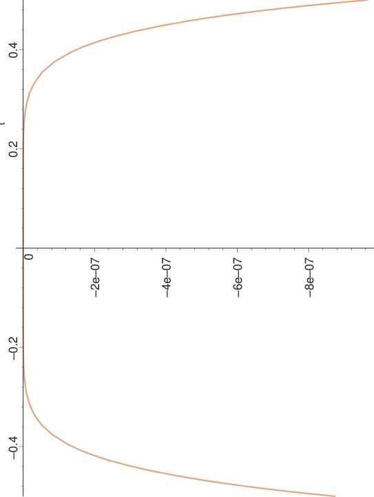
Figure 3: Absolute error in determination of $Z$ using a truncated power series.

When using Hermite polynomials as a set of trial functions, the most sensible definition of inner product is the one under which the Hermite polynomials are orthogonal to each other.

$$\left\langle f|g\right\rangle=\int\limits_{-\infty}^{\infty}f(J)\,g(J)\,e^{-J^{2}/\epsilon^{2}}\,dJ\;.$$

The total accuracy of the computation given by this choice of trial functions is comparable to the accuracy of the solution in terms of the power series and is limited only by the numerical precision of the calculation. Order by order the relative error in determining coefficients $a_{i}$ with respect to epsilon is shown on figure 4. Both graphs show the same solution at different scales. Clearly the precision of the computation of $a_{i}$ decreases at higher orders. From the graph on the left it is evident that $a_{7}$ is determined with an error of $1$ per cent while the graph on the right shows that $a_{5}$ can be calculated more accurately than $5$ parts in $10^{4}$. This trend does not present a problem since the absolute value of the contributions decreases at high orders thus compensating for the loss of accuracy.

Note that the solution is constant in a significant range of values of the parameter. At small values of epsilon this range is limited by numerical precision of the hardware used for the computation. From the graphs it is clear that the calculation becomes numerically unstable when epsilon is set to any value smaller than $0.24$. For large values of the parameter, the range of stability is limited by the number of terms in the approximate solution. If epsilon is set too high, the generating functional can not be accurately approximated at every point in the range $(-\epsilon...+\epsilon)$ by the linear combination of some number (seven in this example) of Hermite polynomials.

The stability property described above is important in computations where a theoretical solution is not available. Then we tune the parameters of a problem to find a stable region which should indicate that we have found a good solution.

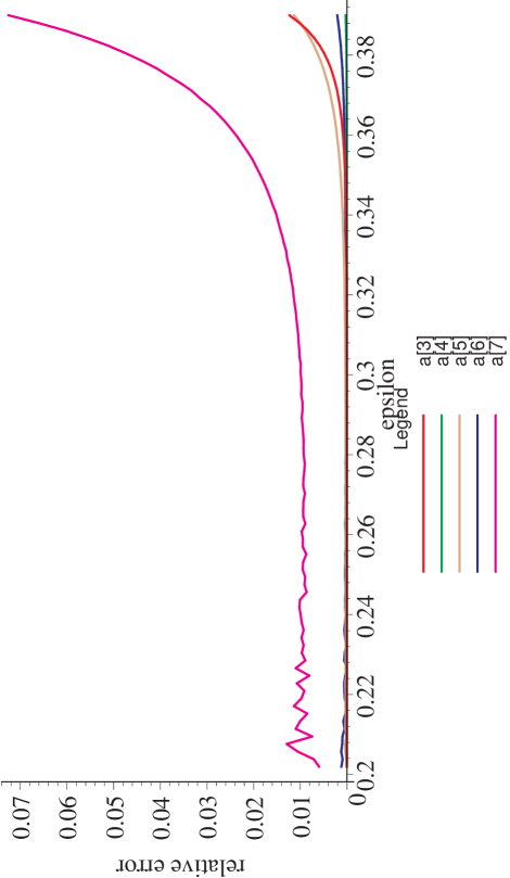
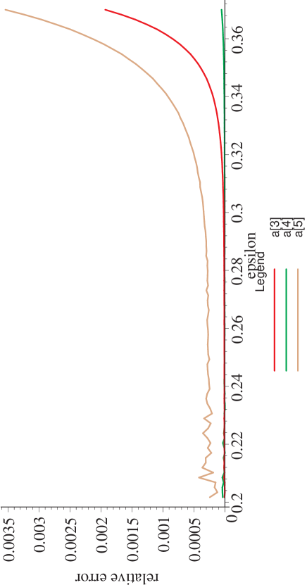
Figure 4: Relative error of Hermite polynomial expansions.

Now, we return to higher dimensions. In order to solve,

$$F\biggl{(}\frac{\delta}{\delta J}\biggr{)}Z[J]=0\;,$$

through numerically approximation, we start with the exact answer in the form:

$$Z[j]=\exp\biggl{\{}a+J(x)\,G(x)+\frac{J\,G^{2}\,J}{2!}+J\,J\,J\,G^{3}+J\,J\,G^{4}\,J\,J+\dotsb\biggr{\}}\;.$$

Here, co-ordinates are only displayed in the linear term and space-time integrations are not shown. Initially, the $G^{i}(x_{1},\dotsc,x_{n})$ can, be anything consistent with the symmetries of the theory. The fact that the zero dimensional model did not have integrations is why it was so simple.

Using the Poincare invariance to produce spectral forms, we conjecture that it should be possible to span the solution space (or a very large part of it) with products of arbitrary two field propagators

$$G_{p}(x-y)=\int\frac{e^{i\,k\,(x-y)}\,a_{p}(K^{2})}{K^{2}-k^{2}}\,d^{4}k\,d^{2}K\;.$$

Thus, we represent $G^{n}$ by all possible graphs with $n$ external lines, all numbers of lines intersecting at any vertex and $a_{p}(K^{2})$ different for each propagator. Important! This is NOT PERTURBATION THEORY. The masses and weights in each of these propagators are arbitrary at this stage. If our conjecture is correct, we have merely exploited the restrictions of relativity and translation invariance in writing this representation. The structure we have written is still extremely complex.

The above expansion inserted into the field equations yields conditions of constraint on $a_{p}(K^{2})$. In general, they are too complicated to solve directly. After all, field theory has not be exactly solved! To proceed, we simplify the problem as follows,

• Truncate the expansion in $J$;

• Limit the number of masses in each propagator;

• Limit the number of graphs considered for each $J$.

We do this in an organized, systematic way, so that after a first guess more terms can be included to iterate on the initial answer. Roughly, our procedure works as follows: Begin by guessing an initial solution $Z_{\text{approx}}[J]$ consistent with space-time, spin and other internal symmetries. Since we have not guessed an exact solution:

$$F\biggl{(}\frac{\delta}{\delta J}\biggr{)}\,\mathcal{Z}_{\text{approx}}[J]\neq 0\;.$$

The idea of Source Galerkin is to require that,

$$\int\,dJ_{1}\dotsb dJ_{n}\,F_{i}(J_{1},\dotsc,J_{n})\,F\biggl{(}\frac{\delta}{\delta J}\biggr{)}\,\mathcal{Z}_{\text{approx}}[J]=0\;,$$

so that $\mathcal{Z}_{\text{approx}}[J]$ satisfies the field equations “on the average”. The number of (in principle arbitrary functions) $F_{i}$ is picked so that all the undetermined weights in $\mathcal{Z}_{\text{approx}}[J]$ are determined.

In general, the equations to be solved are non-linear. Consequently, solutions must be determined in a very careful and systematic manner and parameters must be tuned. Theorems for simpler Galerkin-like approaches promise convergence and we assume this is true for this approach. We have tried this method in many simple models, with amazing accuracy when a check is available. In general, it must be confirmed that the results are stable and convergent. Higher order iterations, while simple in principle, have caused us computational difficulties in practice. While we believe that these problems can be resolved, we have not yet fully demonstrated that our method is practicle in more interesting theories.

2.4 The Nonlinear Sigma Model

Here we give a simple but interesting example of a lowest order SG solution. Calculation to the accuracy obtained in this case is moderately difficult to replicate in Monte Carlo. We have also examined leading order corrections which, as stated, are essential for the proof of validity of the method, and which we will discuss elsewhere. The theory is given by

$$\mathcal{L}=\frac{1}{2}\,\Biggl{\{}\partial_{\mu}\,\phi^{a}(x)\,\partial^{\mu}\,\phi_{a}(x)+\chi(x)\biggl{(}\phi^{a}(x)\,\phi_{a}(x)-\frac{1}{g^{2}}\biggr{)}\Biggr{\}}\;.$$

After the introduction of sources $J^{a}(x)$ and $S(x)$ for canonical and auxiliary fields, one has

$$\mathcal{L}=\frac{1}{2}\,\Biggl{\{}\partial_{\mu}\,\phi^{a}(x)\,\partial^{\mu}\,\phi_{a}(x)-J^{a}(x)\,\phi_{a}(x)+\chi(x)\biggl{(}\phi^{a}(x)\,\phi_{a}(x)-\frac{1}{g^{2}}\biggr{)}-\chi(x)\,S(x)\Biggr{\}}\;.$$

The equations of motion that follow are:

$$\Box\,\frac{\delta Z[J,S]}{\delta J^{a}(x)}-\frac{\delta^{2}Z[J,S]}{\delta S(x)\,\delta J^{a}(x)}-J^{a}(x)\,Z[J,S] =0\;;$$

$$\frac{\delta^{2}Z[J,S]}{\delta J^{a}(x)\,\delta J^{a}(x)}-\frac{1}{g^{2}}\,Z[J,S]-2\,S(x)\,Z[J,S] =0\;.$$

We guess the leading approximation to be

$$Z_{a}[J,S]=Z_{0}\,\exp\Biggl{\{}\frac{1}{2}\,\int J^{a}(x)\,G^{a\,b}(x-y)\,J^{b}(y)\,dx\,dy+\int\chi_{0}\,S(x)\,dx\Biggr{\}}\;.$$

The residues are computed by substituting this expression into the Schwinger Dyson equations,

$$R_{1} =\Box\int G^{a\,b}(x-\xi)\,J^{b}(\xi)\,d\xi-J^{a}(x)-\chi_{0}\int G^{a\,b}(x-\xi)\,J^{b}(\xi)\,d\xi\;$$

$$R_{2} =G^{a\,a}(x-x)+\int G^{a\,b}(x-\xi)\,J^{b}(\xi)\,d\xi\,\int G^{a\,b}(x-\eta)\,J^{b}(\eta)\,d\eta-\frac{1}{g^{2}}-2\,S(x)\;.$$

The Source Galerkin equations can be obtained by requiring that the projections of the residues on the weight functions vanish:

$$\left\langle 1|\left\langle J^{b}(y)|R_{1}(x)\right\rangle_{J}\right\rangle_{S} =0\;;$$

$$\left\langle 1|\left\langle 1|R_{2}\right\rangle_{J}\right\rangle_{S} =0\;;$$

which yield,

$$\Box\,G^{a\,b}(x-y)-\delta^{a\,b}(x-y)-\chi_{0}\,G^{a\,b}(x-y) =0\;;$$

$$G^{a\,a}(0)+\epsilon^{2}\,\int G^{a\,b}(\xi-\eta)\,G^{b\,a}(\eta-\xi)-\frac{1}{g^{2}} =0\;;$$

where, the following definition was used for the inner product

$$\left\langle A|B\right\rangle_{J}=\frac{1}{C_{\epsilon}}\,\int A[J(x)]\,B[J(x)]\,e^{-J^{2}(x)/\epsilon^{2}}\,[dJ]\;.$$

It is straightforward to show that the results obtained here give the same two field Green’s function as the leading order large N expansion.

As indicated, the problems with our method occur at higher orders in the expansion. Since our approach can be represented by arbitrary combinations of Feynman graphs whose masses and coefficients are set by solving Galerkin equations, fast numerical evaluation of these graphs is essential for Source Galerkin to be useful. It is for this reason that we developed a new method to numerically study Feynman graphs.

2.5 Feynman Diagrams

Motivated by our work on the Source Galerkin technique, we have carefully looked at the numerical calculation of Feynman graphs. Historically complicated graphs are evaluated with Monte Carlo methods which take a relatively long time to achieve accurate results. We have have been able to devise a new method for numerically evaluating graphs which is very accurate and very fast, and has considerable promise for complex traditional perturbation calculations (such as the eighth order magnetic moment). The availability of such a method is crucial to fully implementing our Galerkin approach.

We use an approximation to the propagator that reduces graph evaluation to a rapidly convergent multi-dimensional sum.[6] We construct a propagator representation as follows: The cutoff two field propagator, $G_{\Lambda}$

$$G_{\Lambda}(x)=\int\frac{d^{4}p}{(2\,\pi)^{4}}\;\frac{e^{i\,p\,x}}{p^{2}+m^{2}}\,e^{-p^{2}/\Lambda^{2}}\;$$

is written using the Sinc function,

$$S_{k}(h,x)\equiv\frac{\sin(\pi\,(x-k\,h)/h)}{\pi\,(x-k\,h)/h}\;,\quad k\in\mathbb{Z}\;$$

as

$$G_{\Lambda,h}(x) =\frac{m^{2}\,h}{(4\,\pi)^{2}}\,\sum_{k=-\infty}^{\infty}p(k)\,\exp\biggl{[}-\frac{m^{2}\,x^{2}}{4\,C(k)}\biggr{]}$$

$$C(k) =e^{k\,h}+\frac{m^{2}}{\Lambda^{2}}\;,\;p(k)=\frac{e^{k\,h-e^{k\,h}}}{C^{2}(k)}\;.$$

The accuracy of the approximation is tuned by the value of $h$, and typically, the propagator can be approximated to very high accuracy (1 part in $10^{16}$) with fewer than 100 terms in the sum. Inserting this representation of the propagator into the graphical topologies we wish to calculate ensures that all the space-time or momentum integrals are Gaussians and can be performed with ease. The resulting multi-dimensional sum can then be quickly and accurately computed numerically. We have calculated 4th non-trivial order (3 loops) in scalar field theory[9] and successfully responded to challenges to the accuracy and speed of the method. We have computed the QED graphs shown in the diagram on the right[7] as well as a few higher order graphs.

Technical issues with accuracy using an “auto” renormalization scheme have slowed the development of a fully automated implementation of this method to higher order QED graphs. We believe these difficulties are soluble. Moreover, the power of this graphical calculation method gives us reason to believe that we can iterate the SG method to moderate order with relatively small amounts of computer time. If this is true, a much broader range of QFT will be opened to numerical solution with current computer power.

Finally, we note that there is a long history of trying to solve QFT by making approximations to the Schwinger Dyson equations. Our approach is unique because of our way of picking best fits and our systematic procedure based on the powerful way of evaluating arbitrary graphs using the Sync expansion techniques described above. The current power of computers has made it possible to revisit these ideas and institute algorithms which previously would have been useless.

3 Mollified Monte Carlo

The success of Monte Carlo methods is very dependent on the form that the “action” takes. If some terms are not positive (sign problem) or imaginary, or if the action has regions of very rapid oscillation, conventional Monte Carlo approaches will mostly fail. The failed actions are amongst the more interesting ones that we would like to evaluate. As a concrete example, consider symmetry breaking such as was discussed in the SG sections. We saw that to get non-vanishing odd Green’s functions, it was necessary to extend the path integral onto the imaginary axis or, equivalently, to examine actions with negative bare mass terms and half line integrations. In general we would not expect Monte Carlo to be able to handle this. Further it would be very nice if we could, at least in some formal manner, examine actions in Minkowski space, which means we must deal with (carefully defined) complex integrals. Again, we can not do this conventionally. The study of phase structure means looking at actions in regions of high oscillation. Using normal approaches,this is asking for trouble.

Doll and his collaborators [8, 10] have discovered a way of rewriting oscillatory integrals which has the potential to overcome most of these problems and allow Monte Carlo like numerical evaluation. We will outline some of the fairly complex details of this approach in what follows, but it is straightforward to state the general procedure. Basically, we will show by the use of a probability function it is possible to rewrite (mollify) an oscillating path integral, so regions that do not contribute (regions of non-stationary phase) are effectively removed. Next we sample the new integral form using importance functions which are heavily weighted around the stationary phase regions of the mollified integral. This modified Monte Carlo approach will converge even with integrals which originally possessed awful oscillations. In fact, Mollified Monte Carlo (MMC) tends to yield results near to mean field (large N) analytic approaches. The results will also be close to SG expansions picked in our usual way. We have examined this “mollified” approach extensively in zero dimensional field theory and are now trying to use it to solve real theories. While we see rapid convergence in regions of high oscillation, this method is more complex than normal Monte Carlo and will not save any time when used in non-oscillatory problems. Further, it provides no new insight into unquenched fermionic calculations - only the potential of convergence in regions previously not accessible.

We make this more specific by showing some simple examples. Our starting point is a seemingly innocent identity using a probability distribution, We define:

$$\int\,f(x)\,dx \mapsto\int\,\left\langle f(x)\right\rangle_{\epsilon}\,dx\;,$$ (3)

where

$$\left\langle f(x)\right\rangle_{\epsilon} \equiv({f}\ast{P_{\epsilon}})(x)\;,$$ (4)

$$=\int\,P_{\epsilon}(x-y)\,f(y)\,dy\;,$$

with

$$\int\,P_{\epsilon}(x)\,dx =1\;.$$

In this case, the smoothing function is given by $P_{\epsilon}(x)$ which is called a “mollifier” or an “approximate identity”. We use one of the properties of the mollifiers,

$$\left\langle f(x)\right\rangle_{\epsilon}\stackrel{{\scriptstyle\epsilon\to 0}}{{\longrightarrow}}f(x)\;\Rightarrow\;\int\,\left\langle f(x)\right\rangle_{\epsilon}\,dx\stackrel{{\scriptstyle\epsilon\to 0}}{{\longrightarrow}}\int\,f(x)\,dx\;.$$

With this simple averaging method we can build mollified versions of the desired partition functions and Green’s functions, tame oscillations and evaluate previously numerically inaccessible functions.

3.1 Simple example

Let us show how oscillations can be tamed by mollifying the very singular function $\exp(i/x)=\cos(1/x)+i\,\sin(1/x)$.

$$g(x)=\exp(i/x) \;,\quad P_{\epsilon}(x)=\frac{\exp\Bigl{\{}-\frac{1}{2}\,\frac{x^{2}}{\epsilon^{2}}\Bigr{\}}}{\sqrt{2\,\pi\,\epsilon^{2}{\,}}}$$

$$\therefore\;\left\langle g(x)\right\rangle_{\epsilon}=\int_{-\infty}^{\infty}\, \frac{\exp\bigl{\{}-(1/2)\,(x-y)^{2}/\epsilon^{2}\bigr{\}}\,\exp\{i/y\}}{\sqrt{2\,\pi\,\epsilon^{2}{\,}}}\,dy$$

An analogous behavior is seen for the imaginary part. It is quite clear that we have smoothed an essential singularity. We will show that this can be used without loosing information to evaluate Green’s functions.

3.2 Simple example (3D): Gaussian mollifier

We give one more example to show that the above result was not a unique case:

$$f_{m}(x)=\exp(i\,m\,x^{2}) \;,\quad P_{\epsilon}(x)=\frac{\exp\Bigl{\{}-\frac{1}{2}\,\frac{x^{2}}{\epsilon^{2}}\Bigr{\}}}{\sqrt{2\,\pi\,\epsilon^{2}{\,}}}$$

$$\Rightarrow\quad\left\langle f_{m}(x)\right\rangle_{\epsilon} =\frac{\exp\Bigl{\{}\frac{i\,m\,x^{2}}{1-2\,i\,m\,\epsilon^{2}}\Bigr{\}}}{\sqrt{1-2\,i\,m\,\epsilon^{2}{\,}}}$$

Once again, it is easy to see that the surfaces in blue/dark grey (mollified) are less oscillatory than their counterparts (red/light grey). This is quite useful when one starts to think about combining the mollifier technique with the Monte Carlo one and sees that we have tamed this highly oscillatory function for positive and negative values of mass and for real and imaginary contributions. This makes it clear that we should be able to handle general sign problems.

3.3 Application of the Method

Now we can outline the application to Monte Carlo integrals. The method, consists of two basic steps. We start by mollifying (pre-averaging) the integrand. The generating functional is given by,

$$\mathcal{Z}_{\epsilon}[j]=\frac{\displaystyle\int\,\left\langle e^{i\,S(\mathbf{x})-i\,\mathbf{j\cdot x}}\right\rangle_{\epsilon}\,[dx]}{\displaystyle\int\,\left\langle e^{i\,S(\mathbf{x})}\right\rangle_{\epsilon}\,[dx]}\;\;,$$

using the following [Gaussian] mollifier:

$$P_{\epsilon}(\mathbf{y}) =\frac{\exp\Bigl{\{}-\frac{1}{2}\,{\mathbf{y}}^{\mathsf{T}}\cdot(\boldsymbol{\epsilon}^{2})^{-1}\cdot\mathbf{y}\Bigr{\}}}{\sqrt{(2\pi)^{n}\,\det(\boldsymbol{\epsilon}^{2}){\,}}}\;.$$

$$\mathcal{I}_{\epsilon} =\int\left\langle f(\mathbf{x})\,e^{i\,S(\mathbf{x})-i\,\mathbf{j\cdot x}}\right\rangle_{\epsilon}\,[dx]\;,$$

$$\mathcal{I}_{\epsilon} \approx f(\mathbf{x_{0}})\,e^{i\,S(\mathbf{x_{0}})-i\,\mathbf{j\cdot x_{0}}}$$ (5)

$$\int\,\frac{\exp\Bigl{\{}-\frac{1}{2}\,{\mathds{B}}^{\mathsf{T}}\cdot(\mathds{1+{\boldsymbol{\epsilon}}^{\mathsf{T}}\cdot\mathds{S}^{\prime\prime}\cdot\boldsymbol{\epsilon}})^{-1}\cdot\mathds{B}\Bigr{\}}}{\sqrt{\det(\mathds{1}+{\boldsymbol{\epsilon}}^{\mathsf{T}}\cdot\mathds{S}^{\prime\prime}\cdot\boldsymbol{\epsilon}){\,}}}\,[dx]\;,$$

where $\boldsymbol{\epsilon}^{2}$ is the covariance matrix that defines the Gaussian distribution, $\mathds{B}=\boldsymbol{\epsilon\cdot\nabla}S(\mathbf{x})$ and $[\mathds{S}^{\prime\prime}]_{ij}=\partial^{2}S(\mathbf{x})/\partial x_{i}\,\partial x_{j}$. Note, we have suppressed the important point that, in general, the functions under study will have multiple stationary phase points.

The integrals of interest take the form:

$$\mathcal{Z}_{\epsilon}[j]=\frac{\displaystyle\int\,\Biggl{[}\frac{\left\langle e^{i\,S(\mathbf{x})-i\,\mathbf{j\cdot x}}\right\rangle_{\epsilon}}{W(\mathbf{x})}\Biggr{]}\,[dW(\mathbf{x})]}{\displaystyle\int\,\Biggl{[}\frac{\left\langle e^{i\,S(\mathbf{x})}\right\rangle_{\epsilon}}{W(\mathbf{x})}\Biggr{]}\,[dW(\mathbf{x})]}\;\;,$$ (6)

where $W(\mathbf{x})$ is known as the importance function and the MC (Metropolis) sampling is done over this new measure. A reasonable properly biased choice is given by, the result of our saddle-point expansion. Thus:

$$W_{\epsilon}(\mathbf{x})=\left|\frac{\exp\Bigl{\{}i\,S(\mathbf{x_{0}})-\frac{1}{2}\,{\mathds{B}}^{\mathsf{T}}\cdot(\mathds{1+{\boldsymbol{\epsilon}}^{\mathsf{T}}\cdot\mathds{S}^{\prime\prime}\cdot\boldsymbol{\epsilon}})^{-1}\cdot\mathds{B}\Bigr{\}}}{\sqrt{\det(\mathds{1}+{\boldsymbol{\epsilon}}^{\mathsf{T}}\cdot\mathds{S}^{\prime\prime}\cdot\boldsymbol{\epsilon}){\,}}}\right|$$

3.4 Airy Function

The action for this model is given by: $S(x)=x^{3}/3+t\,x$. This is an interesting model because one can explicitly calculate the partition function and compare it with the results coming from our mollified Monte Carlo procedure. Moreover, this model has two stationary phase points and the results we display are from the one in the complex plane which is not accessible with normal Monte Carlo. The quantity of interest is:

$$\mathcal{Z}[t]=\frac{\displaystyle\int_{-\infty}^{\infty}\,\exp\biggl{\{}i\,\frac{x^{3}}{3}+i\,t\,x\biggr{\}}\,dx}{\displaystyle\int_{-\infty}^{\infty}\,\exp\biggl{\{}i\,\frac{x^{3}}{3}\biggr{\}}\,dx}\equiv\frac{\operatorname{Ai}(t)}{\operatorname{Ai}(0)}\;.$$

The graphs below show the behavior of the partition function. In the leftmost one, the oscillatory behavior can be clearly seen and, in the rightmost one, the same behavior is shown (for a fixed $t=-16$, in blue/dark grey) together with the mollified version of the partition function (in red).

It is easy to perform the detailed calculations we outline above to get the pure numerical MMC evaluation of this integral. The results are sensationally accurate and show that in this simple example that we can achieve results not allowable in ordinary Monte Carlo approaches. Further, we have done these calculations for the quartic ultra local theory and achieve similar highly accurate results corresponding to all three solutions.

Conclusions

We have examined two possible numerical methods that could extend the results of normal Monte Carlo approaches. We have demonstrated that, at least in zero dimensional field theory, these methods make sense and have unique and useful properties. We only have glimpses of the validity of either method in higher dimensions. However, the development of the higher dimensional SG analysis has led to a new and very rapid method of doing normal perturbation theory. We expect to be able to push both of our methods considerably further in the next year. However, full confirmation of their usefulness will probably have to wait for work by other groups since, like all numerical quantum field theoretic calculations, large collaborations will be required for hard calculations.

References

- [1] Theta Vacua and Boundary Conditions of the Schwinger-Dyson Equations, S. Garcia, Z, Guralnik and G. Guralnik. hep-th/9612079.
- [2] New numerical methods for quantum field theories on the continuum, P. Emirdag, R. Easther, G. S. Guralnik and S. C. Hahn; Nucl. Phys. Proc. Suppl. 83, 938 (2000). hep-lat/9909122.
- [3] A Test of the Source Galerkin Method, D. Petrov, P. Emirdag, G. S. Guralnik. hep-lat/0208024.
- [4] Alternative Numerical Techniques, G. S. Guralnik, J. Doll, R. Easther, P. Emirdag, D. D. Ferrante, S. Hahn, D. Petrov, D. Sabo. hep-lat/0209127.
- [5] New Numerical Method for Fermion Field Theory, John W. Lawson, G.S. Guralnik; Nucl. Phys. B, 459:612,1996. hep-th/9507131.
- [6] Fast Evaluation of Feynman Diagrams, R. Easther, G. S. Guralnik, S. Hahn; Phys. Rev. D, 61:125001, 2000. hep-ph/9903255.
- [7] Fermions, Gauge Theories, and the Sinc Function Representation for Feynman Diagrams, Dmitri Petrov, Richard Easther, Gerald Guralnik, Stephen Hahn, Wei-Mun Wang; Phys.Rev. D 63:105001, 2001, hep-ph/0010143.
- [8] Stationary Tempering and the Complex Quadrature Problem, Dubravko Sabo, J. D. Doll and D. L. Freeman. J. Chem. Phys., 116(9):3509-3520, March 2002.
- [9] The Sinc Function Representation and Three Loop Master Diagrams, Richard Easther, Gerald Guralnik, Stephen Hahn Phys.Rev. D 63:085017, 2001. hep-ph/9912255.
- [10] Mollified Monte Carlo, D. D. Ferrante, J. Doll, G.S. Guralnik, D. Sabo. hep-lat/0209053.