Beam-size effect in Bremsstrahlung

Abstract

The smallness of the transverse dimensions of the colliding beams leads to suppression of bremsstrahlung cross section. This beam-size effect was discovered and investigated at INP, Novosibirsk. Different mechanisms of radiation are discussed. Separation of coherent and incoherent radiation is analyzed in detail. For linear collider this suppression affects the whole spectrum. It is shown that objections to the subtraction procedure in [9] are groundless.

1 Introduction

The bremsstrahlung process at high-energy involves a very small momentum transfer. In the space-time picture this means that the process occurs over a rather large (macroscopic) distance. The corresponding longitudinal length (with respect to the direction of the initial momentum) is known as the coherence (formation) length $l_{f}$. For the emission of a photon with the energy $\omega$ the coherence length is $l_{f}(\omega)\sim\varepsilon(\varepsilon-\omega)/m^{2}\omega$, where $\varepsilon$ and $m$ is the energy and the mass of the emitting particle ( here the system $\hbar=c=1$ is used).

A different situation arises in the bremsstrahlung process at the electron-electron(positron) collision. For the recoil particle the effect turns out to be enhanced by the factor $\varepsilon^{2}/m^{2}$. This is due to the fact that the main contribution to the bremsstrahlung cross section gives the emission of virtual photon with a very low energy $q_{0}\sim m^{2}\omega/(\varepsilon(\varepsilon-\omega))$ by the recoil particle, so that the formation length of virtual photon is $L_{v}(\omega)=l_{f}(q_{0})=4\varepsilon^{3}(\varepsilon-\omega)/m^{4}\omega$. This means that the effect for the recoil particles appears much earlier than for the radiating particles and can be important for contemporary colliding beam facilities at a GeV range [1].

The special experimental study of bremsstrahlung was performed at the electron-positron colliding beam facility VEPP-4 of Institute of Nuclear Physics, Novosibirsk [2]. The deviation of the bremsstrahlung spectrum from the standard QED spectrum was observed at the electron energy $\varepsilon=1.84~{}$GeV. The effect was attributed to the smallness of the transverse size of the colliding beams. In theory the problem was investigated in [3], where the bremsstrahlung spectrum at the collision of electron-electron(positron) beams with the small transverse size was calculated to within the power accuracy (the neglected terms are of the order $1/\gamma=m/\varepsilon$). After the problem was analyzed in [4], and later on in [5] where some of results for the bremsstrahlung found in [3] were reproduced.

It should be noted that in [3] (as well as in all other papers mentioned above) an incomplete expression for the bremsstrahlung spectrum was calculated. One has to perform the subtraction associated with the extraction of pure fluctuation process. This item will be discussed in Sec.2. In Sec.3 an analysis is given of incoherent radiation in electron-positron linear collider.

2 Mechanisms of Radiation

2.1 Dispersion of momentum transfer

We consider the radiation at head-on collision of high energy electron and positron beams. The properties of photon emission process from a particle are immediately connected with details of its motion. It is convenient to consider the motion and radiation from particles of one beam in the rest frame of other beam (the target beam). In this case the target beam is an ensemble of the Coulomb centers. The radiation takes place at scattering of a particle from these centers. If the target consists of neutral particles forming an amorphous medium, a velocity of particle changes (in a random way) only at small impact distances because of screening. In the radiation theory just the random collisions are the mechanism which leads to the incoherent radiation. For colliding beams significant contributions into radiation give the large impact parameters (very small momentum transfers) due to the long-range character of the Coulomb forces. As a result, in the interaction volume, which is determined also by the radiation formation length (in the longitudinal direction), it may be large number of target particles. Let us note that in the case when the contribution into the radiation give impact parameters comparable with the transverse size of target, the number of particles in the interaction volume is determined by the ratio of the radiation formation length to the mean longitudinal distance between particles.

However, not all cases of momentum transfer should be interpreted as a result of random collisions. One have to exclude the collisions, which are macroscopic certain events. For elaboration of such exclusion we present the exact microscopic momentum transfer to the target particle in the form: ${\bf q}=<{\bf q}>+{\bf q}_{s}$. Here $<{\bf q}>$ is the mean value of momentum transfer calculated according to standard macroscopic electrodynamics rules with averaging over domains containing many particles. The longitudinal size of these domains should be large with respect to longitudinal distances between target particles and simultaneously small with respect to the radiation formation length. The motion of particle in the averaged potential of target beam, which corresponds to the momentum transfer $<{\bf q}>$, determines the coherent radiation. While the term ${\bf q}_{s}$ describes the random collisions which define the process of incoherent radiation (bremsstrahlung). Such random collisions we will call “scattering” since $<{\bf q}_{s}>=0$.

We consider for simplicity the case when the target beam is narrow, i.e.when the parameter $1/q_{min}$ characterizing the screening of Coulomb potential in bremsstrahlung is much larger than the transverse dimensions determining the geometry of problem. When a particle crosses the mentioned domain the transverse momentum transfer to particle is

$$\textbf{q}=\sum_{a=1}^{N}\textbf{q}_{a},\quad\textbf{q}_{a}=2\alpha\frac{\mbox{\boldmath$\varrho$}-\mbox{\boldmath$\varrho$}_{a}}{(\mbox{\boldmath$\varrho$}-\mbox{\boldmath$\varrho$}_{a})^{2}},$$ (1)

where $\alpha$=1/137, $N$ is the number of particles in the domain under consideration of the counter-beam, $\varrho$ is the impact parameter of particle, $\mbox{\boldmath$\varrho$}_{a}$ is the transverse coordinate of Coulomb center. The mean value of momentum transfer is

$$\left\langle\textbf{q}\right\rangle=N\left\langle a|\textbf{q}_{a}|a\right\rangle,\quad\left\langle a|\textbf{q}_{a}|a\right\rangle=\int\textbf{q}_{a}w_{c}(\mbox{\boldmath$\varrho$}_{a})d^{2}\varrho_{a},$$ (2)

here $w_{c}(\mbox{\boldmath$\varrho$}_{a})$ is the probability density of target particle distribution over the transverse coordinates normalized to unity. Then

$$\left\langle\textbf{q}_{s}^{2}\right\rangle=N\left\langle a|\textbf{q}_{a}^{2}|a\right\rangle+N(N-1)\left\langle a|\textbf{q}_{a}|a\right\rangle^{2}-\left\langle\textbf{q}\right\rangle^{2}=N(\left\langle a|\textbf{q}_{a}^{2}|a\right\rangle-\left\langle a|\textbf{q}_{a}|a\right\rangle^{2}).$$ (3)

The same expression for the dispersion of transverse momentum gives the quantum analysis of inelastic scattering of emitting particle on a separate particle of target beam in the domain under consideration

$$\overline{\textbf{q}_{in}^{2}}=\sum_{n\neq a}|\left\langle n|\textbf{q}_{a}|a\right\rangle|^{2}=\sum_{n}\left\langle a|\textbf{q}_{a}|n\right\rangle\left\langle n|\textbf{q}_{a}|a\right\rangle-\left\langle a|\textbf{q}_{a}|a\right\rangle^{2}$$

$$=\left\langle a|\textbf{q}_{a}^{2}|a\right\rangle-\left\langle a|\textbf{q}_{a}|a\right\rangle^{2}.$$ (4)

Granting that $N=n_{z}\Delta z$ we find for the mean value of transverse electric field of target beam

$$\textbf{E}_{\perp}(\mbox{\boldmath$\varrho$},z)=2en_{z}(z)\int\frac{\mbox{\boldmath$\varrho$}-\textbf{x}}{(\mbox{\boldmath$\varrho$}-\textbf{x})^{2}}w_{c}(\textbf{x})d^{2}x$$ (5)

For the rate of variation of function $\left\langle\textbf{q}_{s}^{2}\right\rangle$ we get

$$\frac{d\left\langle\textbf{q}_{s}^{2}\right\rangle}{dz}=4\alpha^{2}n_{z}(z)\left[\int\frac{w_{c}(\textbf{x})d^{2}x}{(\mbox{\boldmath$\varrho$}-\textbf{x})^{2}}-\left(\int\frac{\mbox{\boldmath$\varrho$}-\textbf{x}}{(\mbox{\boldmath$\varrho$}-\textbf{x})^{2}}w_{c}(\textbf{x})d^{2}x\right)^{2}\right].$$ (6)

We don’t discuss here applicability of Eq.(6) at $|\mbox{\boldmath$\varrho$}-\textbf{x}|\leq\lambda_{c}$ (see e.g. Sec.III in [9])

It should be noted that in the kinetic equation which describes the motion of emitting particle

$$\frac{\partial f}{\partial t}+\textbf{v}\frac{\partial f}{\partial\textbf{r}}+\dot{\textbf{p}}\frac{\partial f}{\partial\textbf{p}}=\mathbf{St}f$$ (7)

the value of electric field $\textbf{E}_{\perp}$ (5) determines the coefficient $\dot{\textbf{p}}$ in l.h.s of equation (7) while r.h.s of equation arises due to random collisions and is determined by Eq.(6). The kinetic equation for description of radiation was first employed in [6] and later in [7] and [8]. We consider the case when the mean square angle of multiple scattering during the whole time of beams collision is smaller than the square of characteristic radiation angle. It appears, that this property is sufficient for applicability of perturbation theory to the calculation of the bremsstrahlung probability.

2.2 Main characteristics of particle motion and radiation

One of principal characteristics of particle motion defining the properties of coherent radiation (the beamstrahlung) is the ratio of variation of its transverse momentum to the mass during the whole time of passage across the opposite beam $T$

$$\frac{\Delta{\bf p}_{\perp}}{m}\sim\frac{eE_{\perp}\sigma_{z}}{m}\sim\frac{2\alpha N_{c}\lambda_{c}}{\sigma_{x}+\sigma_{y}}\equiv\delta,$$ (8)

where $N_{c}$ is the number of particles in the opposite beam, $\sigma_{x}$ and $\sigma_{y}$ is its transverse dimensions ($\sigma_{y}\leq\sigma_{x}$), $\sigma_{z}$ is the longitudinal size of opposite beam. The dispersion of particle momentum during time $T$ is small comparing with $m$. It attains the maximum for the coaxial beams:

$$\frac{\left<\textbf{q}_{s}^{2}\right>}{m^{2}}=\gamma^{2}\left<\vartheta_{s}^{2}\right>\sim\frac{8\alpha^{2}N_{c}\lambda_{c}^{2}}{\sigma_{x}\sigma_{y}}L\ll 1,$$ (9)

here $\vartheta_{s}^{2}$ is the square of mean angle of multiple scattering, $L$ is the characteristic logarithm of scattering problem ($L\sim 10$). This inequality permits one to use the perturbation theory for consideration of bremsstrahlung, and to analyze the beamstrahlung independently from the bremsstrahlung.

Another important characteristics of motion is the relative variation of particle impact parameter during time $T$

$$\frac{\Delta\varrho_{i}}{\varrho_{i}}\sim\frac{eE_{\perp}\sigma_{z}^{2}}{\varepsilon\sigma_{i}}\sim\frac{2\alpha N_{c}\lambda_{c}\sigma_{z}}{\gamma(\sigma_{x}+\sigma_{y})\sigma_{i}}\equiv D_{i},$$ (10)

here $i$ is $x$ or $y$. When the disruption parameter $D_{i}\ll 1$, the collision doesn’t change the beam configuration and the particle crosses the opposite beam on the fixed impact parameter. If in addition the parameter $\delta\ll 1$ (this situation is realized in colliders with relatively low energies) then the beamstrahlung process can be calculated using the dipole approximation. The main contribution into the beamstrahlung give soft photons with an energy

$$\frac{\omega}{\varepsilon}\leq\frac{\gamma\lambda_{c}}{\sigma_{z}}\ll 1.$$ (11)

In the opposite case $\delta\gg 1$ the main part of beamstrahlung is formed when the angle of deflection of particle velocity is of the order of characteristic radiation angle $1/\gamma$ and the radiation formation length $l_{m}$ is defined by

$$\frac{eE_{\perp}l_{m}}{m}\sim\frac{2\alpha N_{c}\lambda_{c}l_{m}}{(\sigma_{x}+\sigma_{y})\sigma_{z}}=1,\quad l_{m}=\frac{\sigma_{z}}{\delta};$$ (12)

and the characteristic photon energy is

$$\omega\sim\omega_{m}=\frac{\gamma^{2}}{l_{m}}=\varepsilon\chi_{m},\quad\chi_{m}\equiv 2\alpha N_{c}\gamma\frac{\lambda_{c}^{2}}{(\sigma_{x}+\sigma_{y})\sigma_{z}}(\chi_{m}\ll 1).$$ (13)

Here $\chi=|\mbox{\boldmath$\chi$}|$ is the invariant parameter

$$\mbox{\boldmath$\chi$}=\frac{\gamma}{E_{0}}\left[{\bf E}_{\perp}+{\bf v}\times{\bf H}\right],\quad{\bf E}_{\perp}={\bf E}-{\bf v}({\bf v}{\bf E}),$$ (14)

where $E_{0}=m^{2}/e=1.32\cdot 10^{16}$V/cm, which defines properties of magnetic bremsstrahlung in the constant field approximation (CFA). For applicability of CFA it is necessary that relative variation of  ${\bf E}_{\perp}$ in Eq.(5) was small on the radiation formation length $l_{m}$. As far $l_{m}$ is shorter than $\sigma_{z}$ in $\delta\gg 1$ times the characteristic parameter becomes

$$D_{mi}=D_{i}\frac{l_{m}}{\sigma_{z}}=\frac{D_{i}}{\delta}=\frac{\sigma_{z}}{\gamma\sigma_{i}},~{}(i=x,y)$$ (15)

to that extent. The condition $D_{mi}\ll 1$ is fulfilled in all known cases. The mean number of photons emitted by a particle during the whole time of passage across the opposite beam $T$ is $\left<N_{\gamma}\right>\sim\alpha\delta$, it include the electromagnetic interaction constant. Using the estimate (13) we get an estimate of relative energy loss

$$\frac{\Delta\varepsilon}{\varepsilon}\sim\alpha\delta\chi_{m}~{}(\chi_{m}\ll 1)$$ (16)

In the case $\chi_{m}\ll 1$ (this condition is satisfied in all existing facilities and proposed collider projects) the soft photons with energy $\omega\sim\omega_{m}=\varepsilon\chi_{m}\ll\varepsilon$ are mainly emitted. For $\omega\gg\omega_{m}$ the emission probability is exponentially suppressed. So, such photons are emitted in the bremsstrahlung process only. The boundary photon energy $\omega_{b}$, starting from which the bremsstrahlung process dominates, depends on particular parameters of facility. If $\chi_{m}\sim 1/10$ the energy is $\omega_{b}\sim\varepsilon$. The formation length for $\omega\gg\omega_{m}$ is much shorter than $l_{m}$. On this length the particle deflection angle is small comparing with $1/\gamma$ and one can neglect the variation of transverse beam dimensions (see Eq.(15)). This means that all calculations of bremsstrahlung characteristics can be carried out in adiabatic approximation using local beam characteristics $\sigma_{x,y}(t),{\bf v}(t)$ etc, with subsequent averaging of radiation characteristics over time. Note that actually we performed a covariant analysis and the characteristic parameters are defined in a laboratory frame.

2.3 Separation of coherent and incoherent radiation

As an example we consider the situation when the configuration of beams doesn’t change during the beam collision (the disruption parameter $D\ll 1$), and the total particle deflection angle during intersection of whole beam is small comparing with the characteristic radiation angle $1/\gamma$ (the dipole case). The target beam in its rest frame is the ensemble of classical potentials centers with coordinates ${\bf r}_{a}~{}({\bf x}_{a},~{}z_{a})$ and the transverse coordinate of emitting particle is ${\bf r}_{\perp}$. In the perturbation theory the total matrix element of the radiation process can be written as

$$\textbf{M}(\textbf{r}_{\perp})=\sum_{a=1}^{N_{c}}\textbf{m}(\textbf{r}_{\perp}-\textbf{x}_{a})\exp(iq_{\parallel}z_{a})$$ (17)

We represent the combination $M_{i}M_{j}^{\ast}$ in the form

$$M_{i}M_{j}^{\ast}=\sum_{a=b}m_{i}(\textbf{r}_{\perp}-\textbf{x}_{a})m_{j}(\textbf{r}_{\perp}-\textbf{x}_{b})$$

$$+\sum_{a\neq b}m_{i}(\textbf{r}_{\perp}-\textbf{x}_{a})m_{j}(\textbf{r}_{\perp}-\textbf{x}_{b})\exp(-iq_{\parallel}\left(z_{a}-z_{b})\right).$$ (18)

In the expression Eq.(18) we have to carry out averaging over position of scattering centers. We will proceed under assumption that there are many scattering centers within the radiation formation length $l_{f}=1/q_{\parallel}$

$$N_{f}=n_{z}l_{f}\gg 1,$$ (19)

where for the Gaussian distribution

$$n_{z}=\frac{N_{c}}{\sqrt{2\pi}\sigma_{z}}\exp\left(-\frac{z^{2}}{2\sigma_{z}^{2}}\right),$$ (20)

here $N_{c}$ and $\sigma_{z}$ are introduced in Eq.(8). Note that in the situation under consideration $\varrho_{max}=|\textbf{r}_{\perp}-\textbf{x}_{a}|_{max}\geq\sigma_{t}$, where $\sigma_{t}$ is the characteristic transverse size of target beam. Let us select terms with approximately fixed phase $q_{\parallel}(z_{a}-z_{b})=\phi_{ab}$ in the sum with $a\neq b$ in Eq.(18). If the condition (19) is fulfilled, there are many terms for which the phase variation is small ($\Delta\phi_{ab}\ll 1$). For this reason one can average over the transverse coordinates (${\bf x}_{a},{\bf x}_{b}$) of target particles in Eq.(18) without touching upon the longitudinal coordinates ($z_{a},z_{b}$)

$$M_{i}M_{j}^{\ast}=N_{c}\left\langle m_{i}m_{j}\right\rangle_{\perp}+\left\langle m_{i}\right\rangle_{\perp}\left\langle m_{j}\right\rangle_{\perp}\sum_{a\neq b}\exp(-iq_{\parallel}\left(z_{a}-z_{b})\right)$$

$$=N_{c}\Big{(}\left\langle m_{i}m_{j}\right\rangle_{\perp}-\left\langle m_{i}\right\rangle_{\perp}\left\langle m_{j}\right\rangle_{\perp}\Big{)}+\left\langle m_{i}\right\rangle_{\perp}\left\langle m_{j}\right\rangle_{\perp}\left|\sum_{a}\exp(iq_{\parallel}z_{a})\right|^{2},$$ (21)

where

$$\left\langle m_{i}\right\rangle_{\perp}=\int m_{i}(\textbf{r}_{\perp}-\textbf{x})w_{c}(\textbf{x})d^{2}x,$$

$$\left\langle m_{i}m_{j}\right\rangle_{\perp}=\int m_{i}(\textbf{r}_{\perp}-\textbf{x})m_{j}(\textbf{r}_{\perp}-\textbf{x})w_{c}(\textbf{x})d^{2}x,$$ (22)

here $w_{c}(\textbf{x})$ is the probability density of target particle distribution over the transverse coordinates normalized to unity. In Eq.(21) in the sum with $a\neq b$ we add and subtract the terms with $a=b$. The first term (proportional to $N_{c}$) on the right-hand side of Eq.(21) is the incoherent contribution to radiation (the bremsstrahlung). The second term gives the coherent part of radiation. For Gaussian distribution Eq.(20) performing averaging over the longitudinal coordinate $z_{a}$ one has

$$\left|\sum_{a}\exp(iq_{\parallel}z_{a})\right|^{2}\rightarrow\left|\int_{-\infty}^{\infty}n_{z}\exp(iq_{\parallel}z)dz\right|^{2}=N_{c}^{2}\exp(-q_{\parallel}^{2}\sigma_{z}^{2}).$$ (23)

3 Incoherent Radiation

The correction to photon emission probability due to the small transverse dimensions of colliding beam for unpolarized electrons and photon was calculated in [9] basing on subtraction procedure as in Eq.(21). It is obtained after integration over the azimuthal angle of the emitted photon

$$dw_{1}=\frac{\alpha^{3}}{\pi m^{2}}\frac{\varepsilon^{\prime}}{\varepsilon}\frac{d\omega}{\omega}U(\zeta)F(\omega,\zeta)d\zeta,\quad\zeta=1+\gamma^{2}\vartheta^{2},$$ (24)

where $\vartheta$ is the photon emission angle, $\varepsilon^{\prime}=\varepsilon-\omega$,

$$U(\zeta)=v-\frac{4(\zeta-1)}{\zeta^{2}},~{}v=\frac{\varepsilon}{\varepsilon^{\prime}}+\frac{\varepsilon^{\prime}}{\varepsilon},\quad F(\omega,\zeta)=F^{(1)}(\omega,\zeta)-F^{(2)}(\omega,\zeta),$$

$$F^{(1)}(\omega,\zeta)=\frac{\eta^{2}}{\zeta^{2}}\int\left[K_{0}(\eta\varrho)K_{2}(\eta\varrho)-K_{1}^{2}(\eta\varrho)\right]\varrho\frac{d\Phi(\mbox{\boldmath$\varrho$})}{d\varrho}d^{2}\varrho$$

$$F^{(2)}(\omega,\zeta)=\frac{2\eta^{2}}{\zeta^{2}}\int\left(\int K_{1}(\eta\varrho)\frac{\mbox{\boldmath$\varrho$}}{\varrho}w_{c}({\bf x}-\mbox{\boldmath$\varrho$})d^{2}\varrho\right)^{2}w_{r}({\bf x})d^{2}x,$$ (25)

here

$$\eta=q_{min}\zeta,~{}q_{min}=m^{3}\omega/4\varepsilon^{2}\varepsilon^{\prime},~{}\Phi(\mbox{\boldmath$\varrho$})=\int w_{r}({\bf x}+\mbox{\boldmath$\varrho$})w_{c}({\bf x})d^{2}x,$$ (26)

where $w_{c}({\bf x})$ is defined in (22), $w_{r}({\bf x})$ is the same but for the radiating beam, value $q_{min}$ is defined in c.m.frame of colliding particles. The term $F^{(2)}(\omega,\zeta)$ is the subtraction term. The total probability is $dw_{\gamma}=dw_{0}+dw_{1}$, where $dw_{0}$ is standard QED probability. The analysis in [9] was based on Eqs.(24)-(25).

We considered in [9] the actual case of the Gaussian beams. The Fourier transform was used

$$w({\bf x})=\frac{1}{(2\pi)^{2}}\int d^{2}q\exp(-i{\bf qx})w({\bf q});$$

$$w_{r}({\bf q})=\exp\left[-\frac{1}{2}(q_{x}^{2}\Delta_{x}^{2}+q_{y}^{2}\Delta_{y}^{2})\right],~{}w_{c}({\bf q})=\exp\left[-\frac{1}{2}(q_{x}^{2}\sigma_{x}^{2}+q_{y}^{2}\sigma_{y}^{2})\right],$$ (27)

where as above the index $r$ relates to the radiating beam and the index $c$ relates to the target beam, $\Delta_{y}$ and $\Delta_{x}$ ($\sigma_{y}$ and $\sigma_{x}$) are the vertical and horizontal transverse dimensions of radiating (target) beam. Substituting (27) into Eq.(26) we find

$$\Phi(\mbox{\boldmath$\varrho$})=\frac{\Sigma_{x}\Sigma_{y}}{\pi}\exp[-\varrho_{x}^{2}\Sigma_{x}^{2}-\varrho_{y}^{2}\Sigma_{y}^{2}];~{}\Sigma_{x}^{2}=\frac{1}{2(\sigma_{x}^{2}+\Delta_{x}^{2})},~{}\Sigma_{y}^{2}=\frac{1}{2(\sigma_{y}^{2}+\Delta_{y}^{2})}.$$ (28)

Using the relation $d\sigma_{1}=\Phi^{-1}(0)dw_{1}$ the following expression for the correction to spectrum was found in [9] starting from (24)

$$d\sigma_{1}^{(1)}=\frac{2\alpha^{3}}{m^{2}}\frac{\varepsilon^{\prime}}{\varepsilon}\frac{d\omega}{\omega}f^{(1)}(\omega),~{}f(s)=\frac{\sqrt{\pi}}{2s}(v-8s^{2}){\rm erfc}(s)+4\displaystyle{e^{-s^{2}}}+2{\rm Ei}(-s^{2}),$$

$$f^{(1)}(\omega)=-\frac{1}{\pi\Sigma_{x}\Sigma_{y}}\int_{0}^{2\pi}\frac{d\varphi}{\Sigma_{x}^{-2}\cos^{2}\varphi+\Sigma_{y}^{-2}\sin^{2}\varphi}\int_{0}^{\infty}F_{2}(z)f(s)sds,$$ (29)

$$z^{2}=\frac{s^{2}q_{min}^{-2}}{\Sigma_{x}^{-2}\cos^{2}\varphi+\Sigma_{y}^{-2}\sin^{2}\varphi},~{}F_{2}(x)=\frac{2x^{2}+1}{x\sqrt{1+x^{2}}}\ln(x+\sqrt{1+x^{2}})-1,$$

where Ei($x$) is the exponential integral function and erfc($x$) is the error function. This formula is quite convenient for the numerical calculations.

The subtraction term ($F^{(2)}(\omega,\zeta)$ in (25)) gives for coaxial beams

$$d\sigma_{1}^{(2)}=-\frac{2\alpha^{3}}{m^{2}}\frac{\varepsilon^{\prime}}{\varepsilon}\frac{d\omega}{\omega}J^{(2)}(\omega),$$ (30)

where

$$J^{(2)}(\omega)=\frac{\sqrt{ab}}{\Sigma_{x}\Sigma_{y}}\int_{0}^{\infty}ds_{1}\int_{0}^{\infty}ds_{2}g\left(\frac{q_{min}\sqrt{s}}{2}\right)G(s_{1},s_{2}),$$

$$G(s_{1},s_{2})=\frac{1}{2}\left(\frac{a_{1}a_{2}b_{1}b_{2}}{AB}\right)^{1/2}\left[\frac{a_{1}a_{2}}{A}+\frac{b_{1}b_{2}}{B}\right]$$ (31)

Here the function $g(q)$ is:

$$g(q)=\left(v-\frac{2}{3}\right)\displaystyle{e^{-q^{2}}}-2q^{2}\left[\frac{\sqrt{\pi}}{2q}\left(v-\frac{8}{3}q^{2}\right){\rm erfc}(q)+\frac{4}{3}\displaystyle{e^{-q^{2}}}+{\rm Ei}(-q^{2})\right].$$ (32)

In (31) we introduced the following notations

$$a=\frac{1}{2\Delta_{x}^{2}},\quad b=\frac{1}{2\Delta_{y}^{2}},\quad a_{1,2}=\frac{1}{s_{1,2}+2\sigma_{x}^{2}},\quad b_{1,2}=\frac{1}{s_{1,2}+2\sigma_{y}^{2}},$$

$$A=a_{1}+a_{2}+a,\quad B=b_{1}+b_{2}+b,\quad s=s_{1}+s_{2}.$$ (33)

In the case of narrow beams one has $q_{min}/(\Sigma_{x}+\Sigma_{y})\ll 1$. In this case of coaxial beams $d\sigma_{\gamma}=d\sigma_{0}+d\sigma_{1}$ is

$$d\sigma_{\gamma}=\frac{2\alpha^{3}}{m^{2}}\frac{\varepsilon^{\prime}}{\varepsilon}\frac{d\omega}{\omega}\Bigg{\{}\left(v-\frac{2}{3}\right)\Bigg{[}2\ln\frac{m}{\Sigma_{x}+\Sigma_{y}}+C+2-J_{-}\Bigg{]}+\frac{2}{9}\Bigg{\}},$$ (34)

where

$$J_{-}=\frac{\sqrt{ab}}{\Sigma_{x}\Sigma_{y}}\int_{0}^{\infty}ds_{1}\int_{0}^{\infty}ds_{2}G(s_{1},s_{2})$$ (35)

The dimensions of beams in the experiment [2] were $\sigma_{y}=\Delta_{y}=24~{}\mu m,\sigma_{x}=\Delta_{x}=450~{}\mu m$, so this is the case of flat beams. The estimate for this case gives $J_{-}\simeq(4/3\sqrt{3})\pi\sigma_{y}/\sigma_{x}\ll 1$. This term is much smaller than other terms in (34). This means that for this case the correction to the spectrum calculated in [3] is very small. The parameters of beam in the experiment [11] were (in our notation): $\sigma_{y}=\Delta_{y}=(50\div 58)\mu m$, $\sigma_{x}=\Delta_{x}=(250\div 290)\mu m$. Since the ratio of the vertical and the horizontal dimensions is not very small, the contribution of subtraction term (Eq.(30)) is essential (more than 10%). For details of comparison of experimental data [2], [11] with theory see [9], where we discussed also possible use of beam-size effect for linear collider tuning. It should be noted that for linear collider the condition of strong beam-size effect $\sigma_{y}q_{min}\ll 1~{}(\sigma_{y}\ll\sigma_{x})$ is fulfilled for the whole spectrum. This can be seen in Fig.1, where the lower curve is calculated using Eq.(29) and the subtraction term is very small since $\sigma_{y}/\sigma_{x}<0.01$. As far as the narrow beams are considered in Fig.1, the lower curve is consistent also with Eq.(34). This curve depends on the energy and the transverse sizes of beams. It will be instructive to remind that the analysis in [9] (see Eq.(2.8)) and here is valid if $\chi_{m}/u\ll 1$ (see Eq.(13), $u=\omega/\varepsilon^{\prime}$). The parameter $\chi_{m}$ depends also on number of particles $N_{c}$ and the longitudinal beam size. So, for low $N_{c}$ Fig.1 is valid for any $x$, but for TESLA project ($\chi_{m}$=0.13) it holds in hard part of spectrum only. In fact, the probability of incoherent radiation becomes larger than the probability of coherent radiation only at $x>0.7$ where the lower curve in Fig.1 is certainly applicable.

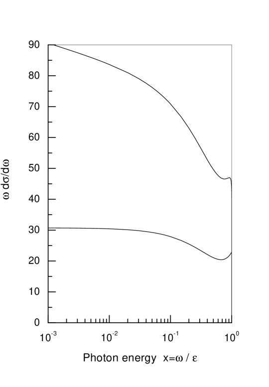
Figure 1: The bremsstrahlung intensity spectrum $\omega d\sigma/d\omega$ in units $2\alpha r_{0}^{2}$ versus the photon energy in units of initial electron energy ($x=\omega/\varepsilon$) for linear collider with beam energy $\varepsilon=250~{}$GeV. The upper curve is the standard QED spectrum. The curve below is calculated with the beam-size effect taken into account for $\sigma_{x}=553nm,\sigma_{y}=5nm$.

Beam-size effect was considered using different approaches which are more or less equivalent formulations of QED perturbation theory where the incident particles consists of wave packets. In [3] the universal method was used which permits to obtain any QED cross section within the relativistic accuracy (up to terms $\sim 1/\gamma$). A “general scheme” in [5] doesn’t fall out the scope of [3] and particular derivation follows method used in [4]. As it was shown above, the subtraction procedure is necessary to extract pure fluctuation process, this was done in [9].

Recently in [10] this subtraction procedure was questioned. An objection is based on correlator Eq.(28) in [10]. If one takes integrals over ${\bf r}$ and ${\bf r}^{\prime}$ from both sides of this correlator, one obtains using Eq.(21) in [10]:$N_{p}^{2}=N_{p}(N_{p}+1)$. It is evident that the last relation as well as correlator Eq.(28) in [10] are not adequate for the discussed problem since the subtraction term is of the same ($\propto N_{p}$)as the relation error. According to [10] (see text before Eq.(19)) the correlator Eq.(28) is obtained as result of “the averaging over fluctuation of particle in the field connected, for example, with the fluctuations of particle positions for many collisions of bunches in a given experiment” (our italics BK). This statement has no respect to the problem under consideration. As it is shown in Secs.2.1 and 2.3 the main aspect is the presence of many scattering centers within the radiation formation length. An analysis in Appendix A confirms this conclusion for radiation in crystals. The reference (Ref.21 in [10]) to the textbooks is senseless because different problems are discussed in these books.

The only correct remark in [10] is that in [9] there was no derivation of the starting formulas. This derivation is given here above. In Sec.2.1 a generic picture of particle motion in the field of counter-beam (in its rest frame) is given. A smooth variation of transverse momentum in an averaged field of counter-beam is considered. It determines the coherent radiation (the beamstrahlung). Along with smooth variation there are the fluctuations of particle velocity due to multiple scattering on the formation length. Just these fluctuations ensure the incoherent radiation (the bremsstrahlung). The mean square of transverse momentum dispersion at multiple scattering on the formation length (see Eqs.(3), (4), (6)) determines the bremsstrahlung probability. The mentioned equations contain both the singular and the subtraction terms accordingly to [9]. In Sec.2.3 we separated the coherent and incoherent parts of radiation explicitly just under the same conditions as in [10]. The result (Eq.(21)) agrees with Eq.(3.6) in [9] which is input formula for analysis in [9].

Appendix A Radiation in crystals

Separation of coherent and incoherent radiation in oriented single crystals was considered using different approaches in [12],[13] and in [14], [15]. We give here a sketch of the analysis in one-chain approximation neglecting correlations due to collision of projectile with different chains. In this case

$$\left\langle\sum_{a\neq b}m_{i}(\textbf{r}_{\perp}-\textbf{x}_{a})m_{j}(\textbf{r}_{\perp}-\textbf{x}_{b})e^{-iq_{\parallel}\left(z_{a}-z_{b}\right)}\right\rangle$$

$$=\left\langle m_{i}\right\rangle_{\perp}\left\langle m_{j}\right\rangle_{\perp}e^{-q_{\parallel}^{2}u^{2}}\sum_{a\neq b}e^{-iq_{\parallel}\left(z_{a}^{(0)}-z_{b}^{(0)}\right)},$$ (A.36)

where $u$ is the amplitude of the thermal vibrations, in averaging over the thermal vibrations we used the distribution

$$w(z_{a})=\frac{1}{\sqrt{2\pi}u}\exp\left(-\frac{(z_{a}-z_{a}^{(0)})^{2}}{2u^{2}}\right).$$ (A.37)

The sum in the r.h.s. of (A.36) one can present as

$$\sum_{a\neq b}\exp(-iq_{\parallel}\left(z_{a}^{(0)}-z_{b}^{(0)})\right)=-N_{c}+\left|\sum_{a}\exp(iq_{\parallel}z_{a}^{(0)})\right|^{2},$$ (A.38)

where

$$\sum_{a}\exp(iq_{\parallel}z_{a}^{(0)})=\sum_{n=-\infty}^{\infty}\exp(inq_{\parallel}d)=2\pi\sum_{k=-\infty}^{\infty}\delta(q_{\parallel}d-2\pi k),$$

$$\left|\sum_{a}\exp(iq_{\parallel}z_{a}^{(0)})\right|^{2}=\frac{N_{c}}{d}2\pi\sum_{k=-\infty}^{\infty}\delta(q_{\parallel}-2\pi\frac{k}{d}),$$ (A.39)

where $d$ is the distance between atoms forming the chain. Substituting Eqs.(A.36)-(A.39) in Eq.(18) we get

$$\left\langle M_{i}M_{j}^{\ast}\right\rangle=N_{c}\left(\left\langle m_{i}m_{j}\right\rangle_{\perp}-\exp(-q_{\parallel}^{2}u^{2})\left\langle m_{i}\right\rangle_{\perp}\left\langle m_{j}\right\rangle_{\perp}\right)$$

$$+N_{c}\frac{2\pi}{d}\exp(-q_{\parallel}^{2}u^{2})\left\langle m_{i}\right\rangle_{\perp}\left\langle m_{j}\right\rangle_{\perp}\sum_{k=-\infty}^{\infty}\delta(q_{\parallel}-2\pi\frac{k}{d}).$$ (A.40)

This expression agrees with Eq.(11) in [12]. The incoherent term in Eq.(A.40) ($\propto N_{c}$) coincide with the incoherent term in Eq.(23) if $q_{\parallel}u\ll 1$. This is true if the condition Eq.(19) ($l_{f}/d\gg 1$) is satisfied.

References

• [1] V.N.Baier and V.M.Katkov, Sov.Phys.Doklady, 17, 1068 (1973).
• [2] A.E.Blinov, A.E.Bondar, Yu.I.Eidelman et al., Preprint INP 82-15, Novosibirsk 1982; Phys.Lett. B113, 423 (1982).
• [3] V.N.Baier, V.M.Katkov, V.M.Strakhovenko, Preprint INP 81-59, Novosibirsk 1981; Sov.J.Nucl.Phys, 36, 95 (1982).
• [4] A.I.Burov and Ya.S.Derbenev, Preprint INP 82-07, Novosibirsk 1982.
• [5] G.L.Kotkin, S.I.Polityko, and V.G.Serbo, Yad.Fiz., 42 692, 925 (1985).
G.L.Kotkin et al., Z.Phys., C39, 61 (1988).
• [6] A.B.Migdal, Phys. Rev., 103, 1811 (1956).
• [7] V.N.Baier, V.M.Katkov, V.M.Strakhovenko, Sov.Phys.JETP, 67, 70 (1988).
• [8] V.N.Baier and V.M.Katkov, Phys. Rev. D57, 3146 (1998).
• [9] V.N.Baier and V.M.Katkov, Phys. Rev. D66, 053009 (2002).
• [10] G.L.Kotkin, and V.G.Serbo, hep-ph/0212102, 2002.
• [11] K.Piotrzkowski, Z.Phys. C67 577 (1995).
• [12] Bazylev V.A, Golovoznin V.V., and Demura A.V. Zhurn.Teor.i Eksp. Fiziki, 92, 1921 (1987).
• [13] Bazylev V.A, and Zhevago N.K.,Radiation from Fast Particles in Solids and External Fields β€œβ€™Nauka’, Moscow, 1987, (in Russian).
• [14] V.N.Baier, V.M.Katkov, V.M.Strakhovenko, phys.stat.sol.(b) 149, 403 (1988).
• [15] V.N.Baier, V.M.Katkov, V.M.Strakhovenko, Electromagnetic Processes at High Energies in Oriented Single Crystals, World Scientific Publishing Co, Singapore, 1998.