Further Evidence for Neutrino Flux Variability from Super-Kamiokande Data

Abstract

While KamLAND apparently rules out Resonant-Spin-Flavor-Precession (RSFP) as an explanation of the solar neutrino deficit, the solar neutrino fluxes in the Cl and Ga experiments vary with solar rotation rates. Added to this evidence, summarized here, a power spectrum analysis of the Super-Kamiokande data reveals (99.9% CL) an oscillation in the band of twice the equatorial rotation frequencies of the solar interior. An $m=2$ magnetic structure and RSFP, perhaps as a subdominant process, would give this effect. Solar cycle data changes are seen, as expected for convection zone modulations.

Recent results from the KamLAND experiment ref:1 seem to confirm the Large-Mixing Angle (LMA) solution to the solar neutrino deficit and rule out the Resonant-Spin-Flavor-Precession (RSFP) explanation ref:2 . On the other hand, there is increasing evidence ref:3 -ref:9 that the solar neutrino flux is not constant as assumed for the LMA solution, but rather it varies with well known solar rotation periods. The solar neutrino situation may be complex, and Spin-Flavor-Precession could be subdominant to LMA, as suggested in ref:10 , or if there is at least one light sterile neutrino even RSFP could be a subdominant process. Since this recent information on solar neutrino variability is not widely known, a brief summary is presented of analyses of radiochemical neutrino data, along with new input from the Super-Kamiokande experiment ref:11 . While the 10-day averages of Super-Kamiokande solar neutrino data ref:12 show no obvious time dependence, a power-spectrum analysis ref:13a displays a strong peak at the frequency $26.57\pm 0.05$ y^-1 (period 13.75 d), where the width of peaks are computed for a probability drop to 10%. The probability of finding this peak (or a stronger peak) by chance within a band specified by twice the near-equatorial rotation frequencies of the solar interior (25.36-27.66 y^-1) is found to be 0.001 (99.9% CL). This frequency is also seen in the radiochemical data.

Whether or not it is the correct interpretation, the RSFP framework provides a simple way to understand the data, and hence it will be used here. The RSFP mechanism, which requires a neutrino transition magnetic moment, provides at least as good a global fit ref:13 ; ref:14 to solar data (which depends mainly on the Super-Kamiokande spectrum) and a better fit to average rates of the individual experiments than does LMA. This is because the neutrino survival probability, while having a resonance pit at a density that suppresses the 0.86 MeV ⁷Be line (as does the Small-Mixing-Angle (SMA) solution), tends at high energies toward 1/2 and hence fits the Super-Kamiokande spectrum, whereas the survival probability goes to unity in the SMA case. Thus, as a subdominant process, it could also improve fits to the data.

A brief review follows of the published evidence for solar neutrino flux variability, put into a coherent neutrino scheme. By analyzing $10^{3}$ simulated data sequences, it was found ref:3 that the variance of the Homestake solar neutrino data ref:15 is larger than expected at the 99.9% CL. A power spectrum analysis ref:3 of the data showed a peak at $12.88\pm 0.02$ y^-1 (28.4 d), compatible with the rotation rate of the solar radiative zone. Four sidebands gave evidence at the 99.8% CL for a latitudinal effect associated with the tilt of the sun’s rotation axis, and the latitude dependence was also seen directly in the data at the 98% CL ref:4 . The GALLEX data ref:16 showed a peak at $13.59\pm 0.04$ y^-1, compatible with the equatorial rotation rate of the deep convection zone. This peak is also in the Homestake data, and a combined analysis of both data sets shows that the 13.59 y^-1 peak is larger than in either data set alone. Comparison ref:7 of the power spectrum for the GALLEX data with a probability distribution function for the synodic rotation frequency as a function of radius and latitude, derived from SOHO/MDI helioseismology data ref:17 , results in Fig. 1. This map shows the rotation frequency coincides with the neutrino modulation in the equatorial section of the convection zone at about 0.8 of the solar radius, $R_{\odot}$. The influence of these rotation frequencies extends even to the corona, since the SXT instrument ref:18 on the Yohkoh spacecraft provides X-ray evidence for two “rigid” rotation rates, one ($13.55\pm 0.02$ y^-1) mainly at the equator, and the other ($12.86\pm 0.02$ y^-1) mainly at high latitudes. These values are in remarkable agreement ref:8 with the neutrino modulation frequencies and also with their equatorial location in one case and non-equatorial in the other; see Fig. 2.

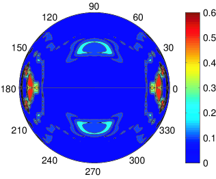
Figure 1: Map of the resonance statistic of the SOHO/MDI helioseismology and GALLEX data on a meridional section of the solar interior. The only high probability areas (red) are lens-shaped sections near the equator, and all others are low probability.

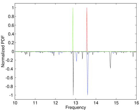
Figure 2: Comparison of normalized probability distribution functions formed from power spectra of data from SXT equator (red), SXT N60-S60 (green), Homestake (black), and GALLEX (blue). Note that the SXT (red) and GALLEX data are equatorial, and the other two are not.

That two dominant frequencies are shown by both coronal X-rays and neutrino flux is a feature of magnetic rotation well known in solar physics. For instance, an analysis ref:19 of the photospheric magnetic field during solar cycle 21 found two dominant magnetic regions: one in the northern hemisphere with synodic rotation frequency $\sim 13.6$ y^-1, and the other in the southern hemisphere with synodic rotation frequency $\sim 13.0$ y^-1. Similarly, an analysis ref:20 of flares during solar cycle 23 found a dominant synodic frequency of $\sim 13.5$ y^-1 for the northern hemisphere and $\sim 12.9$ y^-1 for the southern hemisphere. These and other studies show a strong tendency for magnetic structure to rotate either at about 12.9 y^-1 or at about 13.6 y^-1. Since the sun’s magnetic field is believed to originate in a dynamo process at or near the tachocline, it is possible that some magnetic flux is anchored in the radiative zone just below the tachocline, where the synodic rotation frequency is about 12.9 y^-1, and some just above the tachocline in the convection zone, where the synodic rotation frequency is about 13.6 y^-1. It is also possible that the 12.9 y^-1 frequency results from a latitudinal wave motion in the convection zone excited by structures at or near the tachocline.

An example of latitudinal oscillatory motion of magnetic structures may be the well-known Rieger-type oscillations with frequencies of about 2.4, 4.7, and 7.1 y^-1 ref:21 . These periodicities may be attributed to r-mode oscillations with spherical harmonic indices $\ell=3$, $m=1$,2,3, giving frequencies $\nu=2m\nu_{R}/\ell(\ell+1)$ which are seen in neutrino data ref:3 ; ref:5 ; ref:9 . A joint spectrum analysis ref:9 of Homestake and GALLEX-GNO data yields peaks at 12.88, 2.33, 4.62, and 6.94 y^-1, indicating a sidereal rotation frequency $\nu_{R}=13.88\pm 0.03$ y^-1. While $l\geq 2$ is required, odd$-l$ values have nonzero poloidal velocity at the equator that could move magnetic regions in or out of the neutrino beam to earth.

The difference between the main modulations detected by the Cl and Ga experiments may be explained by the tilt of the solar axis relative to the ecliptic, along with the fact that Cl and Ga neutrinos are produced mainly at quite different radii. The Ga data comes mostly—especially as the fit requires suppressing the ⁷Be line—from $pp$ neutrinos, which originate predominantly at large solar radius ($\sim 0.2$ R_⊙), so that the wide beam of neutrinos detected on earth is insensitive to axis tilt. Thus the beam of neutrinos detected by the Ga experiments exhibits no seasonal variation and can be modulated by the equatorial structure indicated in Fig. 1, leading to the observed frequency at about 13.6 y^-1. On the other hand, the Homestake experiment detects neutrinos produced from a smaller sphere ($\sim 0.05$ R_⊙), so that the axis tilt causes these neutrinos mainly to miss the equatorial structure of Fig. 1 and instead sample nonzero latitudes where the 12.9 y^-1 modulation may occur. Twice a year axis tilt has no effect for these neutrinos, leading to a seasonal variation in the measured flux ref:4 .

The 13.6 y^-1 frequency, located as in Fig. 1, represents a modulation of the $pp$ neutrinos which are at or near the steeply falling edge of the neutrino survival probability. This is close to the RSFP resonance pit suppressing the ${}^{7}\rm{Be}$ neutrinos, which is where the largest value of $\Delta m^{2}/E$ satisfies

$$\Delta m^{2}/E=2\sqrt{2}G_{F}N_{\rm eff},$$ (1)

and is essentially the same as for an MSW resonance ref:23 . For MSW, $N_{\rm eff}=N_{e}$ (the electron density), and for RSFP $N_{\rm eff}=N_{e}-N_{n}$ for Majorana neutrinos, where $N_{n}$ is the neutron density (about $N_{e}/6$ in the region of interest in the Sun). For Dirac neutrinos $N_{\rm eff}=N_{e}-N_{n}/2$, but only Majorana neutrinos provide a fit to solar experimental rates with RSFP ref:13 ; ref:14 , a very important consequence of such a solar solution. Using the $N_{e}$ and $N_{n}$ values at the 0.8 R_⊙ location of Fig. 1 in Eq. 1 results in $\Delta m^{2}/E\sim 10^{-14}$ eV, putting the RSFP resonance pit at the location needed to fit the solar data. $N_{\rm eff}$ varies exponentially with radius and would be quite different for a somewhat changed neutrino modulation frequency.

It is well known that the convection zone magnetic field changes with the solar cycle, so the neutrino modulation features described above are not permanent. It has been argued ref:24 that an RSFP effect would have to be in the radiative zone, where the field does not change with the solar cycle, under the assumption solar cycle variations are not observed. On the contrary, we show here that solar cycle changes play an important role. Variations in neutrino rates are difficult to observe, since changes in field magnitude would be undetectable if the transition remains adiabatic, and even if flux modulation results, average rates may vary only slightly. The feature that is most sensitive to field magnitude or radial variations is the intersection of the very steeply falling $pp$ neutrino spectrum with the falling edge of the RSFP resonance pit. As can be seen in Fig. 3, the 13.6 y^-1 frequency associated with these neutrinos increased in strength from the start of data taking after the solar maximum of 1989.6 to the solar minimum of 1996.8, after which the modulation becomes weak. Also it was during that cycle that the main buildup in the strength of the 12.9 y^-1 oscillation was detected by Homestake. The SXT X-ray data, with which these two frequencies had remarkable agreement ref:8 , also came from that same solar cycle.

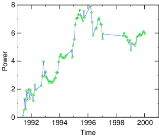
Figure 3: Cumulative Rayleigh power vs. time for the 13.59 y^-1 frequency peak from the GALLEX-GNO data. Note that the power builds up from the start of data taking after the 1990 solar maximum until the 1996.8 solar minimum, after which there is little evidence for that frequency.

Another feature attributable to a time variation of the intersection of the $pp$ spectrum with the edge of the RSFP resonance pit is the appearance of a bimodal flux distribution in the Ga data. This distribution is clearly evident ref:6 during the same solar maximum to solar minimum period when the flux is binned appropriately using individual runs, instead of averages over several data runs. This neutrino flux effect also diminishes after the solar minimum. Adding to the significance of this result is the plot of Fig. 4, which shows that when the end times of runs are reordered according to the phase of the 13.59 y^-1 rotation, the flux values are low in one-half of the cycle and high in the other.

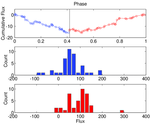
Figure 4: Normalized GALLEX flux measurement runs (prior to 1997) reordered according to the phase of the 13.59 y^-1 solar modulation. The division in phase is made so as to have equal numbers of events in the descending (blue) and ascending (red) parts of the cycle.

It is unfortunate that the Homestake experiment, which detected mainly the ⁸B neutrinos (the only neutrino component registered by Super-Kamiokande) stopped operating at about the time that Super-Kamiokande started. As a result, there is no way to predict from results of other experiments what neutrino flux variation should have been detected by Super-Kamiokande during its operation from May 1996 (near solar minimum) until July 2001 (near solar maximum).

Recently the Super-Kamiokande group released ref:12 flux measurements in 184 bins of about 10 days each. While these measurements vary by $\sim 2$, averaged over all bins their fractional error is $0.14$. Because of the regularity of the binning, the “window spectrum” (the power spectrum of the acquisition times) has a huge peak (power $S>120$) at a frequency of $\nu=35.98$ y^-1 (period 10.15 d). (Note that the probability of obtaining a power of strength $S$ or more by chance at a specified frequency is $e^{-S}$.) This regularity in binning leads to aliasing of the power spectrum of the flux measurements. In a spectrum formed by a likelihood procedure, the strongest peak in the range 0 to 100 y^-1 occurs at $\nu=26.57$ y^-1 ref:13a ; ref:25 with $S=11.26$. In the range 0–40 y^-1, the next strongest peak is at $\nu=9.41$ y^-1 with $S=7.33$. Since $26.57+9.41=35.98$, we infer that the weaker peak (9.41 y^-1) is an alias of the stronger (26.57 y^-1).

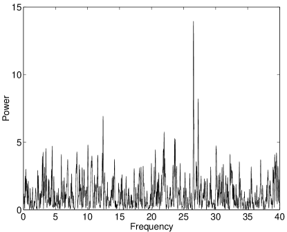
Figure 5: Combined power spectrum of the Super-Kamiokande, SAGE, and GALLEX-GNO data.

Having found this frequency in the high-statistics Super-Kamiokande data, we then examined the power spectrum from a combined analysis of the SAGE ref:26 and GALLEX-GNO data, the sampling time of the Homestake data being too long for this high a frequency. The combined experiments showed a peak at 26.54$\pm 0.05$ y^-1 with $S=5.75$. When combined with the Super-Kamiokande data, we find a peak at 26.54$\pm 0.03$ y^-1 with $S=13.95$, as shown in Fig. 5. There is no significant peak near 9.41 y^-1, further showing this to be an alias frequency.

Since 26.5 y^-1 is within the band of twice the near-equatorial rotation frequencies in the solar interior, this result indicates that some ⁸B neutrinos are experiencing an “$m=2$” structure, two circumferential regions of the magnetic field which differ in strength from the rest. This modulation, unlike the Ga $pp$ threshold effect, is not very deep ($\sim$ 10%). Such oscillations at the harmonic of the rotation frequency are not uncommon in solar data.

The analysis of Super-Kamiokande data, when combined with the results of analyses of Cl and Ga data, yields evidence for variability of the solar neutrino flux. The KamLAND experiment supports the LMA solution, but it could be combined with RSFP. A definitive result on neutrino flux time dependence can be carried out using a combined analysis from all experiments, particularly using one-day bins from all water Cerenkov detectors.

We are indebted to many friends for assistance and helpful discussions. D.O.C. is supported by a grant from the Department of Energy No. DE-FG03-91ER40618, and P.A.S. is supported by grant No. AST-0097128 from the National Science Foundation.

References

- (1) K. Eguchi et al., Phys. Rev. Lett. 90, 021802 (2003).
- (2) C.-S. Lim and W.J. Marciano, Phys. Rev. D 37, 1368 (1988); E.Kh. Akhmedov, Sov. J. Nucl. Phys. 48, 382 (1988) and Phys. Lett. B213, 64 (1988).
- (3) P.A. Sturrock, G. Walther and M.S. Wheatland, Astrophys. J. 491, 409 (1997).
- (4) P.A. Sturrock, G. Walther and M.S. Wheatland, Astrophys. J. 507, 978 (1998).
- (5) P.A. Sturrock, J.D. Scargle, G. Walther and M.S. Wheatland, Astrophys. J. 523, L177 (1999).
- (6) P.A. Sturrock and J.D. Scargle, Astrophys. J. 550, L101 (2000).
- (7) P.A. Sturrock and M.A. Weber, Astrophys. J. 565, 1366 (2002).
- (8) P.A. Sturrock and M.A. Weber, “Multi-Wavelength Observations of Coronal Structure and Dynamics—Yohkoh 10th Anniversary Meeting” (COSPAR Colloquia Series, P.C.H. Martens and D. Cauffman, eds., 2002), p. 323.
- (9) P.A. Sturrock, astro-ph/0304148; hep-ph/0304106.
- (10) E.Kh. Akhmedov and J. Pulido, Phys. Lett. B553, 7 (2003).
- (11) S. Fukuda et al., Phys. Rev. Lett. 86, 5651 (2001).
- (12) M.B. Smy, hep-ex/0206016 and http://www-sk.icrr.u-tokyo.ac.jp/sk/lowe/index.html
- (13) P.A. Sturrock and D.O. Caldwell, Bull. Am. Astron. Soc. 34, 1314 (2002); P.A. Sturrock, hep-ph/0304073, Astrophys. J. (in press).
- (14) M.M. Guzzo and H. Nunokawa, Astropart. Phys. 12, 87 (1999); J. Pulido and E.Kh. Akhmedov, Astropart. Phys. 13, 227 (2000); E.Kh. Akhmedov and J. Pulido, Phys. Lett. B485, 178 (2000); O.G. Miranda, C. Peña-Garay, T.I. Rashba, V.B. Semikoz and J.W.F. Valle, Nucl. Phys. B595, 360 (2001) and Phys. Lett. B521, 299 (2001); J. Pulido, Astropart. Phys. 18, 173 (2002).
- (15) B.C. Chauhan and J. Pulido, Phys. Rev. D 66, 053006 (2002) includes the SNO data in the fits.
- (16) B.T. Cleveland et al., Astrophys. J. 496, 505 (1998).
- (17) W. Hampel et al., Phys. Lett. B447, 127 (1999); M. Altmann et al., Phys. Lett. B490, 16 (2000).
- (18) J. Schou et al., Astrophys. J. 505, 390 (1998).
- (19) S. Tsuneta et al., Solar Phys. 136, 37 (1991).
- (20) E. Antonucci et al., Astrophys. J. 360, 296 (1998).
- (21) T. Bai, Bull. Am. Astron. Soc. 34, 953 (2002).
- (22) E. Rieger et al., Nature 312, 623 (1984); T. Bai, Astrophys. J. 388, L69 (1992).
- (23) L. Wolfenstein, Phys. Rev. D 17, 2369 (1978); Phys. Rev. D 20, 2634 (1979); S.P. Mikheyev and A.Yu. Smirnov, Sov. J. Nucl. Phys. 42, 913 (1985); Nuovo Cimento 9C, 17 (1986).
- (24) A. Friedland and A. Gruzinov, hep-ph/ 0202095.
- (25) A. Milsztajn, hep-ph/0301252 obtained exactly the same result using a different technique in a paper which appeared after the first submittal of the present paper to Phys. Rev. Lett.
- (26) J.N. Abdurashitov et al., Phys. Rev. C 60, 055801 (1999); J. Exp. Theor. Phys. 95, 181 (2002).