Color Superconducting Phases of Cold Dense Quark Matter

B.S., Physics, MIT, 1998
B.S., Electrical Engineering and Computer Science, MIT, 1998
M.Eng., Electrical Engineering and Computer Science, MIT, 1998 Department of Physics
at the Massachusetts Institute of Technology Doctor of Philosophy in Physics June 2003 May 6, 2003

Krishna RajagopalAssociate Professor of Physics

Thomas GreytakChairman, Department Committee on Graduate Students

We investigate color superconducting phases of cold quark matter at densities relevant for the interiors of compact stars. At these densities, electrically neutral and weak-equilibrated quark matter can have unequal numbers of up, down, and strange quarks. The QCD interaction favors Cooper pairs that are antisymmetric in color and in flavor, and a crystalline color superconducting phase can occur which accommodates pairing between flavors with unequal number densities. In the crystalline color superconductor, quarks of different flavor form Cooper pairs with nonzero total momentum, yielding a condensate that varies in space like a sum of plane waves. Rotational and translational symmetry are spontaneously broken. We use a Ginzburg-Landau method to evaluate candidate crystal structures and predict that the favored structure is face-centered-cubic. We predict a robust crystalline phase with gaps comparable in magnitude to those of the color-flavor-locked phase that occurs when the flavor number densities are equal. Crystalline color superconductivity will be a generic feature of the QCD phase diagram, occurring wherever quark matter that is not color-flavor locked is to be found. If a very large flavor asymmetry forbids even the crystalline state, single-flavor pairing will occur; we investigate this and other spin-one color superconductors in a survey of generic color, flavor, and spin pairing channels. Our predictions for the crystalline phase may be tested in an ultracold gas of fermionic atoms, where a similar crystalline superfluid state can occur. If a layer of crystalline quark matter occurs inside of a compact star, it could pin rotational vortices, leading to observable pulsar glitches.

blah

Chapter 1 Introduction

1.1 Overview

In this thesis we shall discuss the behavior of cold quark matter at densities that are relevant for the interiors of compact stars. It is well known that cold dense quark matter is unstable to the formation of a condensate of quark Cooper pairs, making it a color superconductor. Various phases of color superconductivity have been proposed, and in section 1.2 we review the phase diagram of QCD to provide a larger context for a discussion of the color superconducting phases. In section 1.3 we discuss the color-flavor-locked (CFL) color superconductor, the ground state of cold quark matter at very high densities. In section 1.4 we describe how the CFL phase can be disrupted at intermediate densities that are relevant for compact stars. At these intermediate densities, neutral quark matter has unequal numbers of up, down, and strange quarks, and a crystalline color superconducting phase is favored. The crystalline color superconductor has the remarkable virtue of allowing pairing between quarks with unequal Fermi surfaces. Cooper pairs with nonzero total momentum are favored; the condensate spontaneously breaks translational and rotational invariance, leading to gaps which vary periodically in a crystalline pattern as a superposition of plane waves. In section 1.5 we discuss the crystalline phase and look ahead to the detailed calculations of chapters 2 and 3 where we investigate single-plane-wave and multiple-plane-wave crystalline phases, respectively. In section 1.6 we discuss single-flavor color superconductivity, which might occur when there is a very large flavor asymmetry that forbids the crystalline state. We also preview chapter 4, which presents a larger survey of various single-color and single-flavor color superconductors. Many of these are spin-one phases with unusual spectra of elementary excitations. Finally, in section 1.7 we discuss physical contexts in which the crystalline phase may occur with observable consequences. In 1.7.1 we review the astrophysical implications of color superconductivity for compact stars. If a layer of crystalline quark matter occurs inside of a compact star, it could pin rotational vortices, leading to observable pulsar glitches. In 1.7.2, we describe how a crystalline superfluid might be created and detected in a trapped gas of ultracold fermions. These are previews of more detailed discussions of glitches and cold atoms that appear in chapter 5.

1.2 The phase diagram of QCD

In recent years much theoretical and experimental effort has been devoted to understanding the behavior of quantum chromodynamics (QCD) in extreme conditions of very high temperature or density. Because QCD is asymptotically free [1], its high temperature and high density phases are readily described in terms of quark and gluon degrees of freedom [2]. At high temperature, the familiar hadronic phase of QCD gives way to a deconfined plasma of quarks and gluons, in which all the symmetries of the QCD Lagrangian are unbroken [3]. This phase preceded hadronization in the early universe, and efforts are underway to produce and probe this phase in thermalized collisions of relativistic heavy ions at Brookhaven and CERN laboratories [4]. At low temperature and high density, on the other hand, the hadronic phase gives way to a degenerate Fermi system of quarks. Under the influence of the QCD interaction, quarks near the Fermi surface can bind together as Cooper pairs, which condense by the BCS mechanism [5] to form a color superconductor [6, 7, 8, 9, 10, 11, 12, 13, 14, 15, 16, 17, 18]. While not accessible in the laboratory, this cold dense quark matter might occur inside compact stars, with a host of potential astrophysical implications [19].

\psfrag{T}{$T$}\psfrag{primordialuniverse}{\parbox{108.405pt}{primordial \\ universe}}\psfrag{heavyioncollisions}{heavy ion collisions}\psfrag{mu}[tc][tc]{$\mu_{\mbox{\scriptsize quark}}$}\psfrag{muqh}[tc][tc]{$\mu_{qh}$}\psfrag{muunlock}[tc][tc]{$\mu_{\mbox{\scriptsize unlock}}$}\psfrag{compactstars}[tc][tc]{compact stars}\psfrag{1GeV}[tc][tc]{${\textstyle\frac{1}{3}}$GeV}\psfrag{hadrongas}{\parbox{108.405pt}{hadron \\ gas}}\psfrag{hadronliquid}{\parbox{108.405pt}{hadron \\ liquid}}\psfrag{150}[rc][rc]{\parbox{36.135pt}{170 \\ MeV}}\psfrag{crystal}{\parbox{144.54pt}{non-CFL \\ superconductor}}\psfrag{cfl}{\parbox{144.54pt}{CFL \\ superconductor}}\psfrag{quarkgluonplasma}{\parbox{144.54pt}{quark-gluon \\ plasma}}\psfrag{nuclear matter}[rc][rc]{nuclei}\includegraphics[width=397.48499pt]{phasediagram2.eps}

Figure 1.1: Schematic QCD phase diagram with hadronic, plasma, and superconducting phases, as a function of temperature $T$ and chemical potential $\mu_{\mbox{\scriptsize quark}}=\mu_{\mbox{\scriptsize baryon}}/3$. The gray-shaded areas are regions of phenomenological interest.

These various states of QCD fit together in a phase diagram as a function of temperature and chemical potential, as shown in figure 1.1. Let us first consider the temperature axis of this phase diagram. The early universe moved down the vertical axis during the first tens of microseconds after the big bang [20]. The temperature axis can also be studied with lattice simulations, which reveal a transition from a quark-gluon plasma (QGP) to a gas of hadrons at a temperature of about 170 MeV [21]. With realistic quark masses ($m_{s}\gg m_{u,d}\neq 0$), chiral symmetry is explicitly broken everywhere and the transition is a rapid but smooth crossover. Chiral symmetry is (approximately) restored in the QGP phase and broken in the hadronic phase.

Now let us consider the chemical potential axis. Nuclei are droplets of the hadron liquid phase; they sit on the horizontal axis just to the right of the small “curlicue” which is a line of first-order phase transitions between the hadron gas and the hadron liquid (this line terminates at a second-order critical point at a temperature of about 10 MeV) [22]. Moving further to the right along the chemical potential axis, the density increases beyond nuclear density and eventually the nucleons overlap to such an extent that a description in terms of quark degrees of freedom is more suitable. In fact various model calculations suggest that on the horizontal axis there is a first-order transition from the hadronic phase to deconfined quark matter [9, 10, 23, 24, 25, 26, 27]. Starting from this first-order transition at $\mu_{qh}$, a first-order line separating quark and hadron phases extends upwards and to the left, terminating at a second-order critical point before it reaches the temperature axis [23, 24]. In relativistic heavy ion experiments at Brookhaven and CERN, the collided nuclei might follow trajectories in $T$-$\mu$ space like those shown in figure 1.1: the nuclei start at zero temperature, depart from equilibrium during the first moments of collision, then perhaps reappear on the phase diagram at high temperature, thermalizing to create a brief fireball of quark-gluon plasma before expanding and cooling through the quark-hadron transition to produce hadrons.

To the right of $\mu_{qh}$ is the regime of color superconductivity. In this regime deconfined quarks fill large Fermi seas and the interesting physics is that of quarks near their Fermi surfaces (quarks that are deep within Fermi seas are Pauli-blocked and therefore essentially behave as free particles). Pairs of quarks near the Fermi surface that are antisymmetric in color feel an attractive QCD interaction; this is not surprising because at low density and temperature the quarks bind strongly together to form baryons. This attractive interaction makes the system unstable to the formation of a BCS condensate of quark-quark Cooper pairs. Because a pair of quarks cannot be a color singlet, the BCS condensate breaks color gauge symmetry, and the system is a color superconductor.

The phase boundary separating the QGP and color superconducting phases in figure 1.1 occurs at the critical temperature $T_{c}(\mu)$ above which the diquark condensates vanish. This temperature is expected to be a few tens of MeV [18]. Hot protoneutron stars may cool through the color superconducting phase a few seconds after the birth of the star, with interesting implications for neutrino transport in supernovae [28]. Compact stars rapidly cool to temperatures of a few keV and then reside on the chemical potential axis of the QCD phase diagram (at essentially zero temperature) [29]. The chemical potential will vary with depth and the star could be a “hybrid star” with a hadronic mantle and a quark matter core [30, 31, 32, 33]. Because the star temperature is small compared to the critical temperature for color superconductivity, if any quark matter is present then it will be a color superconductor.

At very high densities (far to the right on the phase diagram) the ground state of QCD is the color-flavor-locked (CFL) color superconductor [11, 34, 15, 18]. This is a robust and symmetric phase that is invariant under simultaneous $SU(3)$ rotations in color and flavor. At very high densities the strange quark mass can be neglected and flavor $SU(3)$ is a good symmetry of the QCD Lagrangian. The nonzero strange quark mass explicitly breaks this symmetry and the effect is more pronounced at lower densities. Moving down the chemical potential axis from very high density, this flavor asymmetry can eventually disrupt the CFL phase at an “unlocking” transition [35, 36, 37, 38, 39, 40, 26]. It is uncertain whether unlocking occurs before hadronization. If, as in figure 1.1, we assume that unlocking does occur first, then there is a window in the QCD phase diagram at intermediate density ($\mu_{qh}<\mu<\mu_{\mbox{\scriptsize unlock}}$) for which the ground state of QCD is deconfined quark matter that is not color-flavor-locked.

In unlocked quark matter, pairing should still occur because there is still an attractive interaction between quarks. Any pairing breaks color symmetry so the system remains a color superconductor. In the present work we investigate the novel pairing patterns of quark matter that can occur within this window of non-CFL color superconductivity. We propose that the most favorable candidate is crystalline color superconductivity [41, 42, 43, 44, 45, 46, 47, 48]. Unlocked quark matter has different number densities of $u$, $d$, and $s$ quarks, and we will show that the crystalline phase can accommodate this by forming Cooper pairs with nonzero total momentum. Condensates of this sort spontaneously break translational and rotational invariance, leading to gaps which vary periodically in a crystalline pattern.

1.3 High density and color-flavor-locking

At extremely high densities, the quarks at the Fermi surface have very large momenta and their interactions are asymptotically weak. In this limit, a rigorous theoretical analysis of the QCD ground state is possible using weak-coupling, but non-perturbative, methods of BCS theory [6, 12, 16, 13, 49, 50, 51, 52, 53, 54, 17, 55]. This analysis predicts that at asymptotically-high density, the preferred ground state of QCD is the color-flavor-locked (CFL) color superconductor involving three massless flavors of quarks (at asymptotic densities, one can reasonably neglect the up, down, and strange quark masses). All nine quarks (three flavors, three colors) together form a simple and elegant diquark condensate of the form [11]

$$\langle\psi_{i\alpha a}({\mathbf{x}})\psi_{j\beta b}({\mathbf{x}})\rangle\propto\Delta_{0}\epsilon_{\alpha\beta A}\epsilon_{ijA}(C\gamma_{5})_{ab}$$ (1.1)

with indices for color ($\alpha,\beta$), flavor ($i,j$), and spin ($a,b$). The $\epsilon_{\alpha\beta A}$ tensor indicates that the condensate is an $SU(3)$ color antitriplet of $rg$, $rb$, and $gb$ Cooper pairs. The color $\mathbf{\bar{3}}$ channel is favored because this is the attractive channel for perturbative single-gluon exchange. The $\epsilon_{ijA}$ tensor indicates that the condensate is simultaneously an $SU(3)$ flavor antitriplet of $ud$, $us$, and $ds$ Cooper pairs. The common index $A$ is summed and therefore “locks” color to flavor. The Dirac matrix $C\gamma_{5}$ indicates that the condensate is both rotationally invariant ($J=0$) and parity even. Quarks are paired with the same helicity and opposite momentum; therefore they have opposite spin and form a spin singlet.

The value of the CFL gap $\Delta_{0}$ can be calculated in the asymptotic limit, where the leading interaction is just single gluon exchange. Unfortunately the result can be trusted only at unphysically large chemical potentials, of order $10^{8}$ MeV or higher [56]. Extrapolation to densities of interest for compact stars ($\mu\approx 400$ MeV) is unjustified but yields a gap of about 10-100 MeV. Alternatively, the gap can be calculated by using phenomenological toy models whose free parameters are chosen to give reasonable vacuum physics [9, 10, 23, 11, 14, 15, 57, 58]. For example, one might use a Nambu-Jona-Lasinio (NJL) model in which the interaction between quarks is replaced by a pointlike four-fermion interaction (with the quantum numbers of single-gluon exchange or the instanton interaction), and choose the coupling constant to fit the magnitude of the vacuum chiral condensate at $\mu=0$. It is gratifying that these model calculations also yield gaps of about 10-100 MeV, in agreement with the extrapolation from the asymptotic limit.

The CFL phase has a remarkable pattern of symmetry breaking and elementary excitations [11]. The exact microscopic symmetry group of QCD with three massless flavors is

$$G_{\mbox{\scriptsize microscopic}}=SU(3)_{\mbox{\scriptsize color}}\times SU(3)_{L}\times SU(3)_{R}\times U(1)_{B}$$ (1.2)

where the first factor is the color gauge symmetry, the next two factors are the chiral flavor symmetries, and the last factor is baryon number. Electromagnetism is included by gauging a vector $U(1)$ subgroup of the flavor groups. In the CFL phase, $G_{\mbox{\scriptsize microscopic}}$ is broken to the subgroup

$$G_{\mbox{\scriptsize CFL}}=SU(3)_{\mbox{\scriptsize color}+L+R}\times Z_{2}.$$ (1.3)

The color and chiral flavor symmetries are broken to a “diagonal” global symmetry group of equal $SU(3)$ transformations in all three sectors (color, left-handed flavor, and right-handed flavor). All nine quarks are gapped and the system has nine massive spin-$\frac{1}{2}$ quasiquark excitations that decompose into a octet and a singlet under the diagonal $SU(3)$. The gluon fields produce an SU(3) octet of spin-1 bosonic excitations that acquire a mass by the Meissner-Higgs mechanism. Chiral symmetry is broken and there is an associated octet of massless psuedoscalar bosons. Baryon number is broken to a discrete $Z_{2}$ symmetry in which all the quark fields are multiplied by $-1$; there is an associated massless scalar boson which is the superfluid mode of the CFL phase. The gauge symmetries are completely broken except for a residual $U(1)$ generated by $\tilde{Q}=Q+\frac{1}{\sqrt{3}}T_{8}$ where $Q$ is the electromagnetic charge operator and $T_{8}$ is a generator in the Lie algebra of the $SU(3)$ color group. This $U(1)_{\tilde{Q}}$ symmetry is a gauged subgroup of the unbroken $SU(3)_{\mbox{\scriptsize color}+L+R}$. There is a corresponding $\tilde{Q}$ photon which is a linear combination of the usual photon and the $T_{8}$ gluon (in fact there is just a small admixture of the gluon, so an ordinary magnetic field externally applied to a chunk of CFL matter is mostly admitted as a $\tilde{Q}$ magnetic field and only a small fraction of the flux is expelled by the Meissner effect [59]). All the elementary excitations have integer $\tilde{Q}$ charges.

1.4 Intermediate density and unlocking

The CFL state pairs quarks with different flavors, forming a flavor antitriplet of $ud$, $us$, and $ds$ pairs. As in any BCS state, a quark with momentum ${\mathbf{p}}$ pairs with a quark of momentum $-{\mathbf{p}}$, and the condensate is dominated by those pairs for which each quark is in the vicinity of its Fermi surface: $||{\mathbf{p}}|-p_{F}|\lesssim\Delta_{0}$, where $\Delta_{0}$ is the BCS gap parameter. Since different flavors are paired together, the different flavors must have equal Fermi surfaces for the BCS pairing scheme to work. If the Fermi momenta are different, then it is no longer possible to guarantee that the formation of pairs lowers the free energy: the two fermions in a pair have equal and opposite momentum, so at most one member of each pair can be created at its Fermi surface. This implies that the CFL phase can be disrupted by any flavor asymmetry that would, in the absence of pairing, separate the Fermi surfaces. The nonzero mass of the strange quark has precisely this effect. To understand this, consider noninteracting quark matter with $m_{u}=m_{d}=0$ and $m_{s}\neq 0$. Chemical equilibrium under weak decay reactions requires

$$\mu_{u}=\mu-\frac{2}{3}\mu_{e},\ \ \ \mu_{d}=\mu_{s}=\mu+\frac{1}{3}\mu_{e}$$ (1.4)

where $\mu={\textstyle\frac{1}{3}}\mu_{\mbox{\scriptsize baryon}}$ is the average quark chemical potential, and $\mu_{e}$ is a chemical potential for electrons. With these chemical potentials the noninteracting quarks and electrons fill Fermi seas up to Fermi momenta given by

$$p_{F}^{u,d}=\mu_{u,d},\ \ \ p_{F}^{s}=\sqrt{\mu_{s}^{2}-m_{s}^{2}},\ \ \ p_{F}^{e}=\mu_{e}$$ (1.5)

with corresponding number densities

$$N_{u,d}=\frac{1}{\pi^{2}}\mu_{u,d}^{3},\ \ \ N_{s}=\frac{1}{\pi^{2}}(\mu_{s}^{2}-m_{s}^{2})^{3/2},\ \ \ N_{e}=\frac{1}{3\pi^{2}}\mu_{e}^{3}.$$ (1.6)

Electrical neutrality then requires

$$\frac{2}{3}N_{u}-\frac{1}{3}N_{d}-\frac{1}{3}N_{s}-N_{e}=0.$$ (1.7)

These equations are readily solved and figure 1.2 shows how the Fermi momenta of the quarks and electrons respond as you vary $m_{s}$ at fixed $\mu$. Notice that the effect of the strange quark mass, combined with the requirement of electric neutrality, is to push $p_{F}^{d}$ up and $p_{F}^{s}$ down relative to $p_{F}^{u}$, and at the same time induce a nonzero electron density. To leading order in $m_{s}$ the electron chemical potential is

$$\mu_{e}=\frac{m_{s}^{2}}{4\mu}$$ (1.8)

and the Fermi momenta are

$$p_{F}^{d} = \mu+\frac{m_{s}^{2}}{12\mu}=p_{F}^{u}+\frac{m_{s}^{2}}{4\mu}$$

$$p_{F}^{u} = \mu-\frac{m_{s}^{2}}{6\mu}$$

$$p_{F}^{s} = \mu-\frac{5m_{s}^{2}}{12\mu}=p_{F}^{u}-\frac{m_{s}^{2}}{4\mu}$$ (1.9)

The magnitude of the splitting between Fermi surfaces is $\delta p_{F}=m_{s}^{2}/4\mu$. Notice that decreasing $\mu$ enhances this flavor disparity so the effect is more important at intermediate densities.

\psfrag{mu}[r][r]{$\mu$}\psfrag{ms}[l][l]{$m_{s}$}\psfrag{pfe}[l][l]{$p_{F}^{e}$}\psfrag{pfu}[l][l]{$p_{F}^{u}$}\psfrag{pfd}[l][l]{$p_{F}^{d}$}\psfrag{pfs}[l][l]{$p_{F}^{s}$}\psfrag{pf}[l][l]{$p_{F}$}\psfrag{dpf}[l][l]{$\delta p_{F}$}\includegraphics[width=289.07999pt]{fermi.eps}

Figure 1.2: Fermi momenta for noninteracting electrons and quarks, in a system that is electrically neutral and in weak equilibrium. All three quark Fermi surfaces separate when the strange quark mass is nonzero, with $\delta p_{F}\approx m_{s}^{2}/4\mu$.

The system responds differently when pairing interactions at the Fermi surface are taken into account [37]. At asymptotically high densities, the system is in the CFL state with equal numbers of $u$, $d$, and $s$ quarks. As $\mu$ decreases, the CFL state remains “rigid” with equal numbers of $u$, $d$, and $s$ quarks, despite the presence of a stress which seeks to separate the Fermi surfaces. This rigidity maximizes the binding energy for the Cooper pairs in the CFL phase. The CFL state is the stable ground state of the system only when its negative interaction energy offsets the large positive free energy cost associated with forcing the Fermi seas to deviate from their normal state distributions. The free energy of the CFL state must be compared to that of the unpaired or “normal” state in which the quarks simply distribute themselves in Fermi seas as in figure 1.2. The result is [40]

$$\Omega_{\mbox{\scriptsize CFL}}-\Omega_{\mbox{\scriptsize normal}}\approx-\frac{3}{\pi^{2}}\Delta_{0}^{2}\mu^{2}+\frac{3}{16\pi^{2}}m_{s}^{4}$$ (1.10)

where the negative first term represents the pairing energy gain of the CFL phase, and the positive second term is the cost associated with enforcing equal numbers of $u$, $d$, and $s$ quarks. We have neglected terms in the free energy that are of high order in $\Delta_{0}$ or $m_{s}$. We find that the CFL phase is favored over unpaired quark matter only for [35, 36, 37, 39, 40, 26]

$$\mu>\mu_{\mbox{\scriptsize unlock}}\approx\frac{m_{s}^{2}}{4\Delta_{0}}$$ (1.11)

and the CFL pairing vanishes at a first-order unlocking transition. Notice that the unlocking occurs when the Fermi surface splitting $\delta p_{F}$ in the unpaired phase becomes equal to the gap in the CFL phase: this is consistent with the physical intuition that the CFL phase can “force” the Fermi seas to deviate from their normal state distributions only for $\delta p_{F}<\Delta_{0}$.

In interpreting equation (1.11), recall that the value of the CFL gap is not precisely known: it is of order 10-100 MeV and is also density-dependent. The strange quark mass parameter $m_{s}$ includes the contribution from any $\langle\bar{s}s\rangle$ condensate induced by the nonzero current strange quark mass, making it a density-dependent effective mass. At densities that may occur at the center of compact stars, corresponding to $\mu\sim 400-500$ MeV, $m_{s}$ is certainly significantly larger than the current quark mass, and its value is not well known. In fact, $m_{s}$ decreases discontinuously at the unlocking transition [26]. Thus, the criterion (1.11) can only be used as a rough guide to the location of the unlocking transition in nature. As in figure 1.1 we assume that unlocking occurs before hadronization, so there is a window of intermediate densities where non-CFL quark matter will occur.

It has been proposed [60] that the CFL state may not be completely rigid above the unlocking transition, but may instead respond to the imposed stress by forming a condensate of CFL Goldstone bosons. To respond to the stress the system wants to reduce the number of strange quarks and increase the number of up quarks, as in figure 1.2. Introducing an extra up quark and a strange hole lowers the energy by $\sim m_{s}^{2}/2\mu$, but appears to require the breaking of a pair and therefore involves an energy cost which is of the order of the gap $\Delta_{0}$. However, a down-particle/strange-hole pair has the quantum numbers of a kaon, so the energy cost is actually just the mass of the kaon-like elementary excitation in the CFL phase. The CFL kaon is a pseudo-Goldstone boson which acquires a small mass $m_{K}\sim\Delta_{0}\sqrt{m_{s}m_{d}}/\mu\ll\Delta_{0}$ when nonzero quark masses are introduced which explicitly break chiral symmetry. So the CFL vacuum may lower its free energy by decaying into $K^{0}$ collective modes by the process $0\rightarrow(\overline{us})(du)$. A $K^{0}$ condensate corresponds to a relative rotation of left- and right-handed condensates in flavor space. If kaon condensation occurs, it lowers the free energy of the CFL phase with another term of order $m_{s}^{4}$ in equation (1.10). As a result the 4 in the denominator of (1.11) increases but remains smaller than 5, so this is a relatively minor effect as it concerns unlocking [40].

The unlocking transition was originally studied without the requirement of charge neutrality [35, 36]. It was assumed that $\mu_{u}=\mu_{d}=\mu_{s}=\mu$ and therefore in the unpaired phase the up and down quarks would have equal Fermi momenta $p_{F}^{u}=p_{F}^{d}=\mu$ but the strange quark would have a smaller Fermi momentum $p_{F}^{s}=\sqrt{\mu^{2}-m_{s}^{2}}$, so the system would have a net positive charge density. In this context, $us$ and $ds$ pairing are disrupted at the unlocking transition, but $ud$ pairing should persist because there is no “stress” trying to separate the $u$ and $d$ Fermi surfaces. What is left over is the simple and well-known “2SC” state [9, 10, 18] with a condensate of the form

$$\langle\psi_{i\alpha a}({\mathbf{x}})\psi_{j\beta b}({\mathbf{x}})\rangle\propto\Delta_{0}\epsilon_{\alpha\beta 3}\epsilon_{ij3}(C\gamma_{5})_{ab}.$$ (1.12)

This is quite similar to equation (1.1) for the CFL condensate, except that there is no summation over a common color and flavor antitriplet index $A$. In the 2SC phase the condensate involves only two colors and two flavors. Four of the nine quarks are paired: $rd$ pairs with $gu$, and $ru$ pairs with $gd$. Five quarks are left unpaired (the blue $u$ and $d$ quarks, and all three colors of the strange quark).

In a charge neutral system, however, the 2SC phase is unlikely to occur. As we have seen, imposing charge neutrality in the unpaired phase requires the introduction of an electron chemical potential $\mu_{e}$. This is an isospin chemical potential which separates the up and down Fermi surfaces, so the stress that disrupts $us$ and $ds$ pairing should equally disrupt $ud$ pairing. A detailed calculation confirms that this physical intuition is correct [40, 61]: a calculation of the free energies of charge-neutral CFL, 2SC, and normal (unpaired) states reveals that the 2SC phase is nowhere favored.

Below the unlocking transition, the system is still unstable to the formation of a condensate of Cooper pairs, but the pairing pattern must be something other than CFL or 2SC. Perhaps the most obvious possibility is that the system simply abandons inter-species pairing and forms single-flavor $\langle uu\rangle$, $\langle dd\rangle$, and $\langle ss\rangle$ condensates [8, 62, 63, 64]. Unfortunately these condensates are rather feeble: the gaps are no larger than a few MeV [63, 62], and they could even be much smaller than this [62, 9]. The single-flavor condensates are weak because they must be either symmetric in spin (and therefore $J=1$) or symmetric in color, whereas the QCD interaction favors condensates that are both antisymmetric in spin ($J=0$) and antisymmetric in color. This is easy to understand. The color $\mathbf{\bar{3}}$ channel is the dominant attractive channel, perturbatively (with Coulombic gluons), nonperturbatively (via the instanton interaction), and phenomenologically (from the fact that pairs of valence quarks in a baryon are in a color $\mathbf{\bar{3}}$ state). The $J=0$ channel is enhanced by its rotational symmetry (larger symmetry generally implies more robust pairing).

Condensates that are antisymmetric in color and spin are also antisymmetric in flavor (by the Pauli principle), so the QCD interaction naturally favors inter-species (inter-flavor) pairing. So, inter-species pairing is likely to be favored, but a novel pairing arrangement must be proposed that can accommodate inter-species pairing even at intermediate densities when the different species have different Fermi momenta. The pairing arrangement of the crystalline color superconductor [41, 42, 43, 44, 45, 46, 47, 48] is the most well-studied option, and it is the main emphasis of the current work.

The crystalline phase was originally described by Larkin, Ovchinnikov, Fulde, and Ferrell (LOFF) [65, 66] as a novel pairing mechanism for an electron superconductor with a Zeeman splitting between spin-up and spin-down Fermi surfaces, neglecting all orbital effects of the magnetic perturbation. Quark matter is a more natural setting for the LOFF phase, as it features a “flavor Zeeman effect” with no orbital complications, as a consequence of the large strange quark mass. Cooper pairs in the LOFF phase have nonzero total momentum: a quark with momentum ${\mathbf{p}}$ is paired with a quark with momentum $-{\mathbf{p}}+2{\mathbf{q}}$ such that each quark is near its respective Fermi surface, even though the two Fermi surfaces are disjoint. The magnitude $|{\mathbf{q}}|$ is determined by the separation between Fermi surfaces (we expect $|{\mathbf{q}}|\sim\delta p_{F}$) while the direction $\hat{\mathbf{q}}$ is chosen spontaneously. This generalization of the pairing ansatz (beyond BCS ansätze in which only quarks with momenta which add to zero pair) is favored because it gives rise to a region of phase space where each quark in a pair resides near its respective Fermi surface; as a result, pairs can be created at a low cost in free energy and a condensate can form. In contrast to the BCS phase, where pairing occurs over the entire Fermi surface, LOFF pairing has a restricted phase space. For a given ${\mathbf{q}}$, the quarks that pair are only those in “pairing rings”, one on each Fermi surface; as explained below and in figure 1.3, these circular bands are antipodal to each other and perpendicular to ${\mathbf{q}}$.

As we shall see in chapter 2, the phase space is restricted to the ring-like pairing regions by the formation of “blocking regions” (see figure 2.2) in which pairing is forbidden. Momentum modes inside these blocking regions are occupied by one species of quark but not the other, so pairing cannot occur. Quasiquark excitations are gapless for momenta at the boundaries of these blocking regions, but within the pairing rings the quasiquarks are gapped. Because it has both gapped and gapless quasiparticle excitations, the crystalline state is simultaneously superconducting and metallic.

If each Cooper pair in the condensate carries the same total momentum $2{\mathbf{q}}$, then in position space the condensate varies like a plane wave:

$$\langle\psi({\mathbf{x}})\psi({\mathbf{x}})\rangle\sim\Delta e^{2i{\mathbf{q}}\cdot{\mathbf{x}}}$$ (1.13)

meaning that translational and rotational symmetry are spontaneously broken. This justifies calling it a crystalline color superconductor. Of course, if the system is unstable to the formation of a single plane-wave condensate, then we expect that a superposition of multiple plane waves is still more favorable, leading to a more complicated spatial variation of the condensate:

$$\langle\psi({\mathbf{x}})\psi({\mathbf{x}})\rangle\sim\sum_{{\mathbf{q}}}\Delta_{\mathbf{q}}e^{2i{\mathbf{q}}\cdot{\mathbf{x}}}.$$ (1.14)

Each $\Delta_{\mathbf{q}}$ corresponds to condensation of Cooper pairs with momentum $2{\mathbf{q}}$, i.e. another pairing ring on each Fermi surface. As we add more plane waves, we utilize more of the Fermi surface for pairing, with a corresponding gain in condensation energy. On the other hand, the rings can “interact” with each other: condensation in one mode can enhance or deter condensation in another mode. The true ground state of the system is obtained by exploring the infinite-dimensional parameter space of crystalline order parameters $\{\Delta_{{\mathbf{q}}}\}$ to find that particular crystal structure which is a global minimum of the free energy functional $\Omega[\Delta({\mathbf{x}})]=\Omega(\{\Delta_{{\mathbf{q}}}\})$.

As an aside, it is worth noting that crystalline phases have appeared in other QCD contexts. In their analysis of quark matter with a very large isospin density (with large Fermi momenta for down and anti-up quarks) Son and Stephanov have noted that if the $d$ and $\bar{u}$ Fermi momenta differ suitably, a LOFF crystalline phase will arise [67]. A LOFF crystalline phase can also occur for neutron-proton pairing in asymmetric nuclear matter with a splitting between the neutron and proton Fermi surfaces [68]. Moreover, the LOFF state is not the only crystalline phase that has been investigated: at large baryon number density, pairing between quarks and holes with nonzero total momentum has also been discussed [69, 70, 71, 72]. This results in a chiral condensate which varies in space with a wave number equal to $2\mu$; in contrast, the LOFF phase describes a diquark condensate which varies with a wave number $2|{\mathbf{q}}|$ comparable to $\delta p_{F}$. Several possible crystal structures have been analyzed for the crystalline chiral condensate [72], but this phase is favored at asymptotically high densities only if the number of colors is very large [69], greater than about $N_{c}=1000$ [70, 71]. It may arise at lower densities in QCD with fewer colors, but apparently not in QCD with $N_{c}=3$ [72].

At least two alternatives to the crystalline color superconducting phase have been proposed that also allow pairing between quarks with unequal Fermi surfaces. The first alternative is the deformed Fermi sphere (DFS) superconductor [73]. In this phase, the unequal Fermi surfaces of the two paired species are deformed so that they can intersect, and then pairing can occur in the vicinity of this intersection. The deformations are volume-conserving so that they do not change particle numbers for the two species. The larger Fermi surface has a prolate deformation, while the smaller Fermi surface has an oblate deformation, and pairing occurs along two bands just above and below the equator of each spheroid. The DFS phase breaks rotational symmetry, but unlike the crystalline (LOFF) phase it does not break translational symmetry because the Cooper pairs still have zero total momentum. In both the DFS and LOFF phases the pairing is along circular bands on the Fermi surfaces and therefore the two phases would seem to have similar condensation energies. Meanwhile, in the DFS phase there is also a large kinetic energy cost associated with deforming the Fermi spheres away from their preferred spherical shapes. There is no such cost for the crystalline phase, so we expect the crystalline phase to have a lower free energy.

The second alternative is the “breached-pair” color superconductor [74, 75, 76]. The breached-pair superconductor is translationally and rotationally invariant, in contrast to the crystalline and DFS phases. This state was first encountered by Sarma [74] in the context of an electron superconductor with a Zeeman splitting between the spin-up and spin-down Fermi surfaces, the same context in which the crystalline (LOFF) phase was first proposed. In this historical context it was found that the breached-pair state was never a minimum of the free energy, but recent developments [75, 76] suggest that the breached-pair state might be a stable ground state for pairing between a light species and a heavy species with different Fermi momenta, and therefore might accommodate $us$ and $ds$ pairing in intermediate-density quark matter. In the breached-pair superconductor, the Fermi sea of heavy quarks (Fermi momentum $p_{h}$) is redistributed to accommodate pairing at the light quark Fermi surface (Fermi momentum $p_{l}$). The redistribution has a small energy cost because the heavy quark has a very flat single-particle dispersion relation. For $p_{l}<p_{h}$, heavy quarks are promoted from $|{\mathbf{p}}|\simeq p_{l}$ to $|{\mathbf{p}}|\simeq p_{h}$, creating a “trench” of unoccupied heavy quark states in the interior of the heavy quark Fermi sea. This trench is coincident with the light quark Fermi surface and allows the formation a condensate of Cooper pairs at this surface, a so-called “interior gap” [75]. For $p_{h}<p_{l}$ (the scenario of interest for quark matter), heavy quarks are promoted from $|{\mathbf{p}}|\simeq p_{h}$ to $|{\mathbf{p}}|\simeq p_{l}$, creating a “berm” of occupied heavy quark states far above the heavy quark Fermi sea. This berm is coincident with the light quark Fermi surface and allows the formation of a condensate of Cooper pairs at this surface, a so-called “exterior gap” [76].

The common mechanism in both interior and exterior gap phases is the promotion of a shell of heavy quarks across a momentum “breach” of magnitude $|p_{l}-p_{h}|$, thereby creating a second edge in the momentum distribution of heavy quarks. This edge behaves like a new Fermi surface coincident with the light quark Fermi surface, accommodating the formation of Cooper pairs. The breach is a “blocking region” analogous to the aforementioned blocking regions in the crystalline phase. In the crystalline phase, the blocking regions restrict the pairing to occur on rings and forbid pairing away from these rings. In the breached-pair phase, the blocking region is spherically symmetric and forbids pairing in the breach between $p_{l}$ and $p_{h}$. Just as in the blocking regions of the crystal, momentum modes within the breach are occupied by one species of quark but not the other. In either context, quasiparticle excitations are gapless for momenta at the boundaries of the blocking regions. In the breached-pair state this means that the light quark Fermi surface is gapped while the heavy quark Fermi surface remains ungapped, and the system is simultaneously superconducting and metallic, like the crystalline state. The condensation energy must be weighed against the cost of promotion across the breach: the cost of promotion is small only if the heavy quark dispersion relation is sufficiently flat, so exterior gap $\langle us\rangle$ and $\langle ds\rangle$ condensates can occur only when the strange quark is nonrelativistic. A breached-pair state has been proposed for $ud$ pairing [77], but the preceding argument suggests that this is not a stable ground state. A gapless CFL state, also with breached pairing, has been investigated and was found to be metastable [78]. The evaluation of the energy of breached-pair phases is subtle, and the stability is sensitive to whether a microcanonical (fixed number density) or grand canonical (fixed chemical potential) approach is used [79, 76].

1.5 Crystalline color superconductivity

Crystalline color superconductivity has only been studied in simplified models with pairing between two quark species whose Fermi momenta are pushed apart by a chemical potential difference [41, 42, 48, 46, 47] or a mass difference [45]. We suspect that in reality, in three-flavor quark matter whose unpaired Fermi momenta are split as in (1.9), the pattern of pairing in the crystalline phase will involve $ud$, $us$ and $ds$ pairs, with color and flavor quantum numbers just as in the CFL phase. However, studying the simpler two-flavor problem should elucidate the nature of the crystalline ground state, including its crystal structure. We therefore simplify the color-flavor pattern to one involving massless $u$ and $d$ quarks only, with Fermi momenta split by introducing chemical potentials

$$\mu_{d} = \bar{\mu}+\delta\mu$$

$$\mu_{u} = \bar{\mu}-\delta\mu\ .$$ (1.15)

In this toy model, we vary $\delta\mu$ by hand. In three-flavor quark matter, the analogue of $\delta\mu$ is controlled by the nonzero strange quark mass and the requirement of electrical neutrality and would be of order $m_{s}^{2}/4\mu$ as in (1.9).

The LOFF crystalline phase was originally studied in the context of an electron superconductor with a Zeeman splitting between the spin-up and spin-down Fermi surfaces [65, 66]. The authors considered a magnetic perturbation $\Delta H=h\psi^{\dagger}\sigma_{z}\psi$ but disregarded any orbital effects of the magnetic field. They were seeking to model the physics of magnetic impurities in a superconductor. Magnetic effects on the motion of the electrons [80] and the scattering of electrons off non-magnetic impurities [81, 82] disfavor the LOFF state. Although signs of the BCS to LOFF transition in the heavy fermion superconductor UPd₂Al₃ have been reported [83], the interpretation of these experiments is not unambiguous [84]. It has also been suggested that the LOFF phase may be more easily realized in condensed matter systems which are two-dimensional [85, 86] or one-dimensional [87], both because the LOFF state is expected to occur over a wider range of the Zeeman field $h$ than in three-dimensional systems and because the magnetic field applied precisely parallel to a one- or two-dimensional system does not affect the motion of electrons therein. Evidence for a LOFF phase in a quasi-two-dimensional layered organic superconductor has recently been reported [88].

None of the difficulties which have beset attempts to realize the LOFF phase in a system of electrons in a magnetic field arise in the QCD context of interest to us. Differences between quark chemical potentials are generic and the physics which leads to these differences has nothing to do with the motion of the quarks. We therefore expect the original analysis of LOFF (without the later complications added in order to treat the difficulties in the condensed matter physics context) to be a good starting point.

In our two-flavor model, we shall take the interaction between quarks to be pointlike, with the quantum numbers of single-gluon exchange. This $s$-wave interaction is a reasonable starting point at accessible densities but is certainly not appropriate at asymptotically high density, where the interaction between quarks (by gluon exchange) is dominated by forward scattering. The crystalline color superconducting state has been analyzed at asymptotically high densities in Refs. [46, 47]. We expect a qualitatively different crystalline phase in this asymptotic regime, but this may not be relevant for densities of interest for compact star physics.

With this astrophysical context in mind, it is also appropriate for us to work at zero temperature. Compact stars that are more than a few minutes old are several orders of magnitude colder than the critical temperature (of order tens of MeV) for CFL or crystalline color superconductivity. The crystalline color superconductor has been studied at finite temperature, and the critical temperature is given by $T_{c}/\Delta_{(T=0)}\simeq 0.44$ [42] (a result previously known in the historical LOFF context [89]). It is interesting that this differs from the usual BCS relation $T_{c}/\Delta_{(T=0)}\simeq 0.57$ [5]. The critical temperatures for the CFL and single-flavor color superconductors also differ from the BCS result [64].

Now let us consider how the crystalline phase occurs in our two-flavor model. Starting at ${\delta\mu}=0$, the system forms a BCS superconductor with gap $\Delta_{0}$. In fact this BCS superconductor is precisely the 2SC phase of equation (1.12): the Cooper pairs are color antisymmetric (red pairs with green) and flavor antisymmetric (up pairs with down). The blue quarks are left unpaired. The up and down Fermi surfaces are coincident. As we begin to increase ${\delta\mu}$, the system exhibits a “rigidity” analogous to that of the CFL phase: despite the imposed stress ${\delta\mu}$, the gap stays constant and the Fermi surfaces remain coincident. The BCS state is the stable ground state of the system only when its negative interaction energy offsets the large positive free energy cost associated with forcing the Fermi seas to deviate from their normal state distributions. The free energy of the BCS state, relative to that of of the normal state in which the quarks simply distribute themselves in Fermi seas with $p_{F}^{u}=\mu_{u}$ and $p_{F}^{d}=\mu_{d}$, is approximately

$$\Omega_{\mbox{\scriptsize BCS}}-\Omega_{\mbox{\scriptsize normal}}\approx-\frac{1}{\pi^{2}}\Delta_{0}^{2}\bar{\mu}^{2}+\frac{2}{\pi^{2}}{\delta\mu}^{2}\bar{\mu}^{2}$$ (1.16)

where the first term is the negative pairing energy of the BCS state, and the second term is the cost associated with enforcing equal numbers of up and down quarks in the presence of the imposed stress ${\delta\mu}$. This result is exact only in the weak-coupling limit in which the gap $\Delta_{0}\ll\bar{\mu}$. This expression (1.16) should be compared to equation (1.10) for the free energy of the neutral CFL phase with the imposed stress of a nonzero $m_{s}$. When ${\delta\mu}$ reaches a critical value

$${\delta\mu}_{1}\approx\frac{1}{\sqrt{2}}\Delta_{0}=(0.7071\cdots)\Delta_{0},$$ (1.17)

the BCS phase “breaks” and the Fermi surfaces separate (again, the expression is exact only in the weak coupling limit in which $\Delta_{0}\ll\bar{\mu}$). This is the two-flavor analogue of the CFL unlocking transition. (Bedaque [38] has investigated the mixed phase associated with this first-order transition, where the unpaired blue quarks also play a role.) This result was first derived by Clogston and Chandrasekhar [90] in the context of an electron superconductor with a Zeeman splitting.

For ${\delta\mu}>{\delta\mu}_{1}$, the up and down quarks have unequal Fermi surfaces and a crystalline state is possible. In the simplest LOFF state, up quarks with momentum ${\mathbf{p}}$ are paired with down quarks with momentum $-{\mathbf{p}}+2{\mathbf{q}}$. Each Cooper pair carries the same total momentum $2{\bf q}$. The allowed phase space for ${\mathbf{p}}$ is determined by the requirement that each quark in the Cooper pair should sit near its Fermi surface, i.e.

$$||{\mathbf{p}}|-\mu_{u}|\lesssim\Delta\ \ \ \mbox{and}\ \ \ ||-{\mathbf{p}}+2{\mathbf{q}}|-\mu_{d}|\lesssim\Delta$$ (1.18)

where $\Delta$ is the LOFF gap parameter. This phase space corresponds to a circular band on each Fermi surface as shown figure 1.3. As indicated in the figure, the bands are perpendicular to the spontaneously chosen direction $\hat{\mathbf{q}}$ for the total momentum of each Cooper pair. The magnitude $|{\mathbf{q}}|\equiv q_{0}$ is determined energetically from the separation between Fermi surfaces. We shall find that the relation is $q_{0}\approx 1.20{\delta\mu}$.

\psfrag{muu}[r][r]{$\mu_{u}$}\psfrag{mud}[l][l]{$\mu_{d}$}\psfrag{p}[l][l]{${\mathbf{p}}$}\psfrag{mp}[r][r]{$-{\mathbf{p}}$}\psfrag{p2q}[r][r]{$-{\mathbf{p}}+2{\mathbf{q}}$}\psfrag{pp}[r][r]{${\mathbf{p}}^{\prime}$}\psfrag{mpp}[l][l]{$-{\mathbf{p}}^{\prime}$}\psfrag{pp2q}[l][l]{$-{\mathbf{p}}^{\prime}+2{\mathbf{q}}$}\psfrag{2q}[c][c]{$2{\mathbf{q}}$}\psfrag{psiu}[c][l]{$\psi_{u}$}\psfrag{psid}[c][l]{$\psi_{d}$}\includegraphics[width=252.94499pt]{rings.eps}

Figure 1.3: The LOFF pairing geometry for Cooper pairs with total momentum $2{\mathbf{q}}$. The dashed and solid spheres are the up and down quark Fermi surfaces, respectively. An up quark with momentum ${\mathbf{p}}$ (or ${\mathbf{p}}^{\prime}$) near its Fermi surface pairs with a down quark with momentum $-{\mathbf{p}}+2{\mathbf{q}}$ (or $-{\mathbf{p}}^{\prime}+2{\mathbf{q}}$) near its Fermi surface. The pairing is strongest for up quarks in a band centered on the dashed ring shown on the up Fermi surface, and down quarks in a band centered on the solid ring shown on the down Fermi surface.

It is useful to discuss the various scales involved in the problem. The BCS gap $\Delta_{0}$ can be thought of as the fundamental energy scale for physics at the Fermi surface. If we consider the weak coupling limit in which $\Delta_{0}\ll\bar{\mu}$, then the two scales are cleanly separated and all the other Fermi-surface energy scales in the problem (i.e. $|{\mathbf{q}}|$, ${\delta\mu}$, and the LOFF gap $\Delta$) should be proportional to the fundamental scale $\Delta_{0}$. We achieve this by taking a“double scaling” limit in which we choose to hold ${\delta\mu}/\Delta_{0}$ fixed while taking the $\Delta_{0}/\bar{\mu}\rightarrow 0$ limit. In this double scaling limit, $|{\mathbf{q}}|/\Delta_{0}$ and $\Delta/\Delta_{0}$ also stay fixed. In fact, every dimensional quantity for the Fermi-surface physics stays fixed as “measured” in units of $\Delta_{0}$. If we fail to take the double scaling limit, instead keeping ${\delta\mu}/\bar{\mu}$ fixed as $\Delta_{0}/\mu\rightarrow 0$, we would not find crystalline color superconductivity at weak coupling [91]. We will not always work in the double scaling limit (see, for example, chapter 2), but we will often quote analytic results that are exact in this limit (as we did in equation 1.17). In the double scaling limit, ${\delta\mu}\ll\bar{\mu}$ and the two Fermi surfaces in figure 1.3 are very close together. The opening angles $\psi_{u}$ and $\psi_{d}$ of the two pairing bands become degenerate and take on the value

$$\psi_{0}\approx 2\cos^{-1}\left(\frac{{\delta\mu}}{|{\mathbf{q}}|}\right)\approx 2\cos^{-1}\frac{1}{1.20}=67.1^{\circ}.$$ (1.19)

The radial thickness of each pairing band is of order $\Delta$, while the angular width is $\delta\psi\sim\Delta/\sqrt{|{\mathbf{q}}|^{2}-{\delta\mu}^{2}}\sim 1.5\Delta/{\delta\mu}$. If we use double scaling then both $\psi_{0}$ and $\delta\psi$ are constant because $|{\mathbf{q}}|/\Delta_{0}$, ${\delta\mu}/\Delta_{0}$, and $\Delta/\Delta_{0}$ are all held constant while $\Delta_{0}\rightarrow 0$. Hereafter, when we speak of the “weak coupling limit” we shall always mean the double scaling limit.

If all the Cooper pairs in the condensate have the same nonzero total momentum $2{\mathbf{q}}$, then the condensate varies like a single plane wave in position space, as in equation (1.13). In chapter 2 we present a careful study of this single plane wave condensate, the simplest example of a LOFF phase. We show that there is a range of ${\delta\mu}$ in which quark matter is unstable to the spontaneous breaking of translational invariance by the formation of a plane wave condensate. Of course, once one has demonstrated an instability to the formation of a plane wave, it is natural to expect that the state which actually develops has a crystalline structure consisting of multiple plane waves, as in equation (1.14). In chapter 3 we investigate this possibility. Larkin and Ovchinnikov in fact argue that the favored configuration is a crystalline condensate which varies in space like a one-dimensional standing wave, $\cos(2{\mathbf{q}}\cdot{\mathbf{r}})$. Such a condensate vanishes along nodal planes [65]. Subsequent analyses suggest that the crystal structure may be more complicated. Shimahara [85] has shown that in two dimensions, the LOFF state favors different crystal structures at different temperatures: a hexagonal crystal at low temperatures, square at higher temperatures, then a triangular crystal and finally a one-dimensional standing wave as Larkin and Ovchinnikov suggested at temperatures that are higher still. In three dimensions, the question of which crystal structure is favored was unresolved [92]. Our analysis, shown in chapter 3, suggests that the favored crystal structure in three dimensions is face-centered-cubic.

The crystalline states appear for ${\delta\mu}>{\delta\mu}_{1}$. In chapter 2 we will show that the simplest LOFF state, a single plane wave condensate, can occur in an interval ${\delta\mu}_{1}<{\delta\mu}<{\delta\mu}_{2}$. At ${\delta\mu}_{2}$ there is a second-order transition from LOFF to the normal state (unpaired quarks). The second-order point occurs at

$${\delta\mu}_{2}\approx(0.7544\cdots)\Delta_{0}$$ (1.20)

where this relation is exact in the weak coupling limit (the numerical coefficient is known exactly; it is the solution of a simple transcendental equation). At the second-order phase transition, $\Delta/\Delta_{0}\rightarrow 0$ and $|{\bf q}|/\Delta_{0}$ tends to a nonzero limit, which we shall denote $q_{0}/\Delta_{0}$, where $q_{0}\simeq 0.90\Delta_{0}\simeq 1.20\delta\mu_{2}$. Near the second-order phase transition, the quarks that participate in the crystalline pairing lie on thin circular rings on their Fermi surfaces that are characterized by an opening angle $\psi_{0}\simeq 2\cos^{-1}({\delta\mu}_{2}/q_{0})\simeq 67.1^{\circ}$ and an angular width $\delta\psi$ that is of order $\Delta/{\delta\mu}$ and therefore tends to zero as $\Delta/\Delta_{0}\rightarrow 0$. At $\delta\mu_{1}$ there is a first-order phase transition at which the LOFF solution with gap $\Delta$ is superseded by the BCS solution with gap $\Delta_{0}$. (The analogue in three-flavor QCD would be a LOFF window in $m_{s}^{2}/\mu$, with CFL at lower $m_{s}^{2}/\mu$ (higher density) and unpaired quark matter at higher $m_{s}^{2}/\mu$ (lower density).) These results are summarized in figure 1.4, where we have shown the free energies and gaps for the competing BCS, plane-wave LOFF, and unpaired quark matter phases (the figure also shows the gap and free energy for the multiple-plane-wave LOFF state, which we discuss below). Keep in mind that this figure is just a qualitative sketch which exaggerates the size of the plane-wave LOFF window $[{\delta\mu}_{1},{\delta\mu}_{2}]$. Quantitative plots are shown in figure 2.4 in chapter 2. In the vicinity of the second-order critical point ${\delta\mu}_{2}$, our mean-field analysis yields a gap and free energy for the plane-wave state that obey simple power-law relations

$$\Delta_{\mbox{\scriptsize pw}}\propto\sqrt{{\delta\mu}_{2}-{\delta\mu}},\ \ \ \Omega_{\mbox{\scriptsize pw}}\propto-({\delta\mu}_{2}-{\delta\mu})^{2}$$ (1.21)

with the expected mean field theory critical exponents for a second-order transition.

\psfrag{delta}[rc][rc]{$\Delta$}\psfrag{omega}[rc][rc]{$\Omega$}\psfrag{deltaomega}[rc][rc]{$-\frac{\mu^{2}\Delta_{0}^{2}}{\pi^{2}}$}\psfrag{deltabcs}{$\Delta_{\mbox{\scriptsize BCS}}$}\psfrag{omeganormal}{$\Omega_{\mbox{\scriptsize normal}}\equiv 0$}\psfrag{omegabcs}{$\Omega_{\mbox{\scriptsize BCS}}$}\psfrag{omegapw}[lc][lc]{$\Omega_{\mbox{\scriptsize pw}}$}\psfrag{omegaxtal}[lc][lc]{$\Omega_{\mbox{\scriptsize xtal}}$}\psfrag{delta0}{$\Delta_{0}$}\psfrag{deltamu}{${\delta\mu}$}\psfrag{dm1}[tc][tc]{${\delta\mu}_{1}$}\psfrag{dm2}[tc][tc]{${\delta\mu}_{2}$}\psfrag{dmp}[tc][tc]{${\delta\mu}_{1}^{\prime}$}\psfrag{dms}[tc][tc]{${\delta\mu}_{*}$}\psfrag{deltapw}[lc][lc]{$\Delta_{\mbox{\scriptsize pw}}$}\psfrag{deltaxtal}[lc][lc]{$\Delta_{\mbox{\scriptsize xtal}}$}\includegraphics[width=397.48499pt]{omegadelta2.eps}

Figure 1.4: Free energies and gaps for competing states: normal, BCS, and single and multiple plane wave crystalline phases (“pw” and “xtal”, respectively). For the plane wave state, the LOFF interval is $[{\delta\mu}_{1},{\delta\mu}_{2}]\approx[0.707\Delta_{0},0.754\Delta_{0}]$ ($\Delta_{0}$ is the BCS gap) and the transitions to BCS and normal states are first and second order, respectively. For the multiple plane wave (crystalline) state, the LOFF interval is $[{\delta\mu}_{1}^{\prime},{\delta\mu}_{*}]$ and both transitions are first order. Note that the plane wave state is exaggerated (compare figure 2.4). In reality $({\delta\mu}_{2}-{\delta\mu}_{1})\ll({\delta\mu}_{*}-{\delta\mu}_{1}^{\prime})$ and the crystalline state is much more favorable than the plane wave state.

Proceeding beyond just a single plane wave might seem to be a daunting task. We have to explore the infinite-dimensional parameter space of crystalline order parameters $\{\Delta_{{\mathbf{q}}}\}$ to find the unique crystal structure that is a global minimum of the free energy. However, we can exploit the fact that there is a second-order point ${\delta\mu}_{2}$ which indicates the onset of plane-wave instability in the system. In the vicinity of this second-order point, we can express the free energy as a Ginzburg-Landau potential; the potential is written as a series expansion of the exact free energy in powers of the order parameters $\{\Delta_{{\mathbf{q}}}\}$.

In chapter 3 we explicitly construct the Ginzburg-Landau potential and apply it to a large survey of candidate crystal structures. The Ginzburg-Landau calculation finds many crystal structures that are much more favorable than the single plane wave (1.13). For many crystal structures, the calculation actually predicts a strong first-order phase transition, at some $\delta\mu_{*}\gg\delta\mu_{2}$, between unpaired quark matter and a crystalline phase with a $\Delta$ that is comparable in magnitude to $\Delta_{0}$. Once $\delta\mu$ is reduced to $\delta\mu_{2}$, where the single plane wave would just be beginning to develop, these more favorable solutions already have very robust condensation energies, perhaps even comparable to that of the BCS phase. Therefore they can even compete with the BCS phase and move the position of the first-order transition between BCS and LOFF to a new point ${\delta\mu}_{1}^{\prime}<{\delta\mu}_{1}$. All of this is shown schematically in figure 1.4. These results are exciting, because they suggest that the crystalline phase is much more robust than previously thought. However, they cannot be trusted quantitatively because the Ginzburg-Landau analysis is only controlled in the limit $\Delta\rightarrow 0$, and we find a first-order phase transition to a state with $\Delta\neq 0$.

Even though it is quite a different problem, we can look for inspiration to the Ginzburg-Landau analysis of the crystallization of a solid from a liquid [93]. There too, a Ginzburg-Landau analysis predicts a first-order phase transition, and thus predicts its own quantitative downfall. But, qualitatively it is correct: it predicts the formation of a body-centered-cubic crystal and experiment shows that most elementary solids are body-centered-cubic (BCC) near their first-order crystallization transition.

Thus inspired, let us look at how the Ginzburg-Landau calculation will proceed. We can start by writing down the most general expression for the Ginzburg-Landau potential that is consistent with translational and rotational symmetry. We will include only the modes on the sphere $|{\mathbf{q}}|=q_{0}=1.2{\delta\mu}$ since these are the modes that become unstable at ${\delta\mu}_{2}$. To order $\Delta^{6}$, the expression looks like

$$\Omega(\{\Delta_{\mathbf{q}}\}) \propto \sum_{{\mathbf{q}},|{\mathbf{q}}|=q_{0}}\alpha\Delta_{\mathbf{q}}^{*}\Delta_{\mathbf{q}}+\frac{1}{2}\sum_{\square}J(\square)\Delta_{{\mathbf{q}}_{1}}^{*}\Delta_{{\mathbf{q}}_{2}}\Delta_{{\mathbf{q}}_{3}}^{*}\Delta_{{\mathbf{q}}_{4}}$$ (1.22)

$$+\frac{1}{3}\sum_{\hexagon}K(\hexagon)\Delta_{{\mathbf{q}}_{1}}^{*}\Delta_{{\mathbf{q}}_{2}}\Delta_{{\mathbf{q}}_{3}}^{*}\Delta_{{\mathbf{q}}_{4}}\Delta_{{\mathbf{q}}_{5}}^{*}\Delta_{{\mathbf{q}}_{6}}+\cdots.$$

Odd powers are not allowed because the potential is invariant under $U(1)$ baryon number (which multiples every $\Delta_{\mathbf{q}}$ by a common phase). The symbol $\square$ represents a set of four equal-length vectors $({\mathbf{q}}_{1},{\mathbf{q}}_{2},{\mathbf{q}}_{3},{\mathbf{q}}_{4})$, $|{\mathbf{q}}_{i}|=q_{0}$, with ${\mathbf{q}}_{1}-{\mathbf{q}}_{2}+{\mathbf{q}}_{3}-{\mathbf{q}}_{4}=0$, i.e. the four vectors are joined together to form a closed (not necessarily planar) figure. Similarly, the symbol $\hexagon$ represents a set of six equal-length vectors $({\mathbf{q}}_{1},\ldots,{\mathbf{q}}_{6})$, $|{\mathbf{q}}_{i}|=q_{0}$, with ${\mathbf{q}}_{1}-{\mathbf{q}}_{2}+{\mathbf{q}}_{3}-{\mathbf{q}}_{4}-{\mathbf{q}}_{5}+{\mathbf{q}}_{6}=0$, i.e. the six vectors form a closed “hexagon”. We sum only over closed sets of ${\mathbf{q}}$-vectors because otherwise the Ginzburg-Landau potential, expressed in position space as a functional $\Omega[\Delta({\mathbf{x}})]$, would not be translationally invariant. Rotational invariance implies that the coefficients $J(\square)$ and $K(\hexagon)$ are the same for any two shapes related by a rigid rotation.

The quadratic coefficient $\alpha$ changes sign at ${\delta\mu}_{2}$ showing the onset of the LOFF plane-wave instability: $\alpha\approx({\delta\mu}-{\delta\mu}_{2})/{\delta\mu}_{2}$. If there was no interaction between the different modes, they would just simply all condense at once, because they would all become unstable at the second-order point. The answer is more complicated than this because condensation in one mode can enhance or deter condensation in another mode. This interaction between modes is implemented in our Ginzburg-Landau potential by the higher order terms involving multiple modes; thus the coefficients $J$, $K$, $\ldots$ characterize the interactions between modes and thereby determine the crystal structure.

As we shall see in chapter 3, these coefficients can actually be calculated from the microscopic theory, as loop integrals in a Nambu-Gorkov formalism. So for a candidate crystal structures with all $\Delta_{\mathbf{q}}$’s equal in magnitude, we can evaluate aggregate Ginzburg-Landau quartic and sextic coefficients $\beta$ and $\gamma$ as sums over all rhombic and hexagonal combinations of the ${\mathbf{q}}$’s:

$$\beta=\sum_{\square}J(\square),\ \ \ \gamma=\sum_{\hexagon}K(\hexagon).$$ (1.23)

Then for a crystal consisting of $P$ plane waves we obtain

$$\Omega(\Delta)\propto P\alpha\Delta^{2}+\frac{1}{2}\beta\Delta^{4}+\frac{1}{3}\gamma\Delta^{6}+\cdots$$ (1.24)

and we can then compare crystals by calculating $\beta$ and $\gamma$ to find the structure with the lowest $\Omega$.

Evaluating the quadratic coefficient $\alpha$ determines the location of the plane-wave instability point, i.e. the value of ${\delta\mu}_{2}$. It also tells us that $|{\mathbf{q}}|\simeq 1.20{\delta\mu}$, which means that each pairing ring has an opening angle of $67.1^{\circ}$, as in equation (1.19). As mentioned above, on its own the quadratic term indicates that adding more plane waves (i.e. adding more pairing rings to the Fermi surface) always lowers the free energy. But this conclusion is modified by the higher order terms in two important ways:

1. Crystal structures with intersecting pairing rings are strongly disfavored. Recall that each ${\mathbf{q}}$ is associated with pairing among quarks that lie on one ring of opening angle $\psi_{0}\simeq 67.1^{\circ}$ on each Fermi surface. We find that any crystal structure in which such rings intersect pays a large free energy price. Therefore the favored crystal structures are those that feature a maximal number of rings “packed” onto the Fermi surface without intersections. No more than nine rings of opening angle $67.1^{\circ}$ can be packed on a sphere without intersections [94, 95].

2. Crystal structures are favored if they have a set of ${\mathbf{q}}$’s that allow many closed combinations of four or six vectors, leading to many terms in the $\sum_{\square}$ and $\sum_{\hexagon}$ summations in equation (1.22). Speaking loosely, “regular” structures are favored over “irregular” structures. All configurations of nine nonintersecting rings are rather irregular, whereas if we limit ourselves to eight rings, there is a regular choice which is favored by this criterion: choose eight ${\bf q}$’s pointing towards the corners of a cube. In fact, a deformed cube which is slightly taller or shorter than it is wide (a cuboid) is just as good.

These qualitative arguments are supported by the quantitative results of our Ginzburg-Landau analysis, which do indeed indicate that the most favored crystal structure is a cuboid that is very close to a cube. This crystal structure is so favorable that the coefficients $\beta$ and $\gamma$ in the Ginzburg-Landau potential (equation (1.24)) are large and negative. In fact, we find several crystal structures with negative coefficients, but the cube has by far the most negative $\beta$ and $\gamma$. In other words, starting at the origin in the space of crystalline order parameters $\{\Delta_{{\mathbf{q}}}\}$, the “steepest descent” in free energy is achieved by moving in the direction of the cube structure. Our Ginzburg-Landau potential is unbounded from below, so our analysis is unable to discover the actual free energy minimum or the value of the gap at which this minimum occurs. But we can reasonably presume that the lowest free energy and largest gap are achieved by moving in the direction of steepest descent. We could go on, to order $\Delta^{8}$ or higher, until we found a Ginzburg-Landau free energy for the cube which is bounded from below. However, we know that this free energy would give a strongly first-order phase transition, meaning that the Ginzburg-Landau analysis would anyway not be under quantitative control. A better strategy, then, is to use the Ginzburg-Landau analysis to understand the physics at a qualitative level, as we have done. We understand qualitatively what features of the eight-plane-wave solution make it most favorable, so the next step is to take this as an ansatz, solve the gap equation, and thus obtain a bounded free energy without making a Ginzburg-Landau approximation. This calculation is still in progress, but in figure 1.5 we show what the bounded free energy might look like (solid curve), compared with the unbounded Ginzburg-Landau free energy (dotted curve). The series of plots shows how the unbounded free energy indicates a first order transition: for ${\delta\mu}>{\delta\mu}_{2}$ the quadratic coefficient $\alpha$ is positive: increasing $\Delta$ at fixed ${\delta\mu}$, the free energy should first turn upwards, then downwards under the influence of the negative quartic and sextic terms, then eventually it will turn upwards again because it must be bounded from below. The resulting curve can thus generate a first-order transition as ${\delta\mu}$ is varied, as shown in the figure. For comparison the dashed line shows the free energy of the plane wave crystal (with $\beta,\gamma>0$), which demonstrates a typical second order transition.

\psfrag{Omega1}[lc][lc]{$\Omega({\delta\mu}>{\delta\mu}_{*})$}\psfrag{Omega2}[lc][lc]{$\Omega({\delta\mu}={\delta\mu}_{*})$}\psfrag{Omega3}[lc][lc]{$\Omega({\delta\mu}={\delta\mu}_{2})$}\psfrag{Omega4}[lc][lc]{$\Omega({\delta\mu}<{\delta\mu}_{2})$}\psfrag{Delta}{$\Delta$}\includegraphics[width=209.58255pt]{eplot1.eps}

\psfrag{Omega1}[lc][lc]{$\Omega({\delta\mu}>{\delta\mu}_{*})$}\psfrag{Omega2}[lc][lc]{$\Omega({\delta\mu}={\delta\mu}_{*})$}\psfrag{Omega3}[lc][lc]{$\Omega({\delta\mu}={\delta\mu}_{2})$}\psfrag{Omega4}[lc][lc]{$\Omega({\delta\mu}<{\delta\mu}_{2})$}\psfrag{Delta}{$\Delta$}\includegraphics[width=209.58255pt]{eplot2.eps}

\psfrag{Omega1}[lc][lc]{$\Omega({\delta\mu}>{\delta\mu}_{*})$}\psfrag{Omega2}[lc][lc]{$\Omega({\delta\mu}={\delta\mu}_{*})$}\psfrag{Omega3}[lc][lc]{$\Omega({\delta\mu}={\delta\mu}_{2})$}\psfrag{Omega4}[lc][lc]{$\Omega({\delta\mu}<{\delta\mu}_{2})$}\psfrag{Delta}{$\Delta$}\includegraphics[width=209.58255pt]{eplot3.eps}

\psfrag{Omega1}[lc][lc]{$\Omega({\delta\mu}>{\delta\mu}_{*})$}\psfrag{Omega2}[lc][lc]{$\Omega({\delta\mu}={\delta\mu}_{*})$}\psfrag{Omega3}[lc][lc]{$\Omega({\delta\mu}={\delta\mu}_{2})$}\psfrag{Omega4}[lc][lc]{$\Omega({\delta\mu}<{\delta\mu}_{2})$}\psfrag{Delta}{$\Delta$}\includegraphics[width=209.58255pt]{eplot4.eps}

Figure 1.5: Schematic free energies for the FCC crystal (solid line) and plane wave (dashed line), showing how they support first and second order phase transitions, respectively. The dotted line is the unbounded Ginzburg-Landau expression for the free energy of the FCC crystal.

The eight ${\bf q}$’s of our most-favored crystal structure are the eight shortest vectors in the reciprocal lattice of a face-centered-cubic crystal. Therefore, we find that $\Delta({\mathbf{x}})\sim\langle\psi({\mathbf{x}})\psi({\mathbf{x}})\rangle$ exhibits face-centered-cubic symmetry. Explicitly,

$$\Delta({\mathbf{x}}) = 2\Delta\Biggl{[}\cos\frac{2\pi}{a}(x+y+z)+\cos\frac{2\pi}{a}(x-y+z)$$ (1.25)

$$+\cos\frac{2\pi}{a}(x+y-z)+\cos\frac{2\pi}{a}(-x+y+z)\Biggr{]}\ ,$$

where the lattice constant (i.e. the edge length of the unit cube) is

$$a=\frac{\sqrt{3}\pi}{|{\mathbf{q}}|}\simeq\frac{4.536}{{\delta\mu}}\simeq\frac{6.012}{\Delta_{0}}\ ,$$ (1.26)

where the last equality is valid at ${\delta\mu}={\delta\mu}_{2}$ and where $\Delta_{0}$ is the gap of the BCS phase that would occur at ${\delta\mu}=0$. A unit cell of the crystal is shown in Fig. 1.6. The figure clearly reveals a face-centered-cubic structure. Like any crystal, the FCC crystalline color superconductor should have phonon modes which are Goldstone bosons of spontaneously broken translation symmetry. Casalbuoni et al have formulated an effective theory for the LOFF phonons [48].

\psfrag{0}{\small 0}\psfrag{0.25}{\small 0.25}\psfrag{0.5}{\small 0.5}\psfrag{0.75}{\small 0.75}\psfrag{1}{\small 1}\includegraphics[width=289.07999pt]{unitcell_bm.ps}

Figure 1.6: A unit cell of the LOFF face-centered-cubic crystal. The gray planes are surfaces where $\Delta({\mathbf{x}})=0$. The darker surfaces are contours where $\Delta({\mathbf{x}})=+4\Delta$, and the lighter surfaces are contours where $\Delta({\mathbf{x}})=-4\Delta$.

1.6 Single-flavor color superconductivity

If the Fermi momenta of the $u$, $d$, and $s$ quarks are very far apart then the system has no choice but to abandon inter-species pairing and form single-flavor $\langle uu\rangle$, $\langle dd\rangle$, and $\langle ss\rangle$ condensates. In the two-flavor context of section 1.5, with a splitting ${\delta\mu}$ between the $u$ and $d$ Fermi surfaces, single-flavor pairing will occur for ${\delta\mu}>{\delta\mu}_{*}$. At ${\delta\mu}_{*}$ there is a first-order “crystallization” transition between the single-flavor state and the crystal state with $ud$ pairing. The value of the first-order point ${\delta\mu}_{*}$ is not known; if it were known we could estimate that an analogous crystallization transition will occur in three-flavor neutral quark matter when the Fermi momentum splitting $\delta p_{F}$ approaches $2{\delta\mu}_{*}$, i.e. when

$$\delta p_{F}=\delta p_{F}^{*}\approx\frac{m_{s}^{2}}{4\mu_{*}}\sim 2{\delta\mu}_{*}.$$ (1.27)

(The factor of two occurs because in our notation $p_{F}^{d}-p_{F}^{u}=\delta p_{F}=2{\delta\mu}$). We expect that ${\delta\mu}_{*}$ is appreciably larger than $\Delta_{0}$, which implies that $\mu_{*}$ is appreciably smaller than $\mu_{\mbox{\scriptsize unlock}}$. Crystalline quark matter occurs in the interval between $\mu_{*}$ and $\mu_{\mbox{\scriptsize unlock}}$. If $\mu_{*}$ is below the hadronization point $\mu_{qh}$ then single-flavor quark matter is unlikely to occur and the crystalline phase will occupy the entire interval between hadronization and unlocking in the QCD phase diagram (figure 1.1). Otherwise, there may be a window just above the hadronization point in which single-flavor pairing is possible.

The structure of a single-flavor $\langle uu\rangle$ condensate (flavor index 1) is [62]

$$\langle\psi_{i\alpha a}({\mathbf{x}})\psi_{j\beta b}({\mathbf{x}})\rangle\propto\Delta\epsilon_{\alpha\beta 3}\delta_{i1}\delta_{j1}(C\gamma_{3})_{ab}$$ (1.28)

with indices for color ($\alpha,\beta$), flavor ($i,j$), and spin ($a,b$). The condensate is antisymmetric in color (as usual, the color $\mathbf{\bar{3}}$ channel is favored because this is the attractive channel for the QCD interaction). Only two of the three colors pair; the choice of the index 3 for the color tensor $\epsilon_{\alpha\beta 3}$ is arbitrary and excludes the blue quarks from pairing. The condensate is obviously symmetric in flavor. By the Pauli principle it is also symmetric in Dirac indices. It is a $J=1$ (vector) condensate that breaks rotational symmetry: the Dirac matrix $C\gamma_{3}$ in equation (1.28) indicates that the condensate has spontaneously chosen the 3 direction in position space. The condensate is parity even. The quarks are paired with opposite helicity (LR pairing) and opposite momentum; therefore they have parallel spin and form a ($s=1,m=\pm 1$) spin triplet state.

The gap parameter $\Delta$ can be calculated using an NJL model with a four-fermion interaction vertex [62]. These calculations are shown in chapter 4. Unfortunately the value of the gap is drastically sensitive to the details of the effective interaction and to the chemical potential. It could be as large as 1 MeV, or orders of magnitude smaller (see the dash-dotted line in figure 4.2). For $\mu$ of 400 to 500 MeV, the NJL calculation predicts a gap that ranges from 0.1 to 10 keV (this illustrates the sensitivity to the chemical potential). The calculation is also very model dependent. In figure 4.2 the gap is calculated using an NJL model with pointlike magnetic gluons. Calibrated to give the same CFL gap, a different NJL model that includes pointlike electric and magnetic gluons predicts a much larger gap (by about a factor of 10); with an instanton interaction, no gap is predicted at all (the channel is flavor symmetric and there is no interaction with an instanton vertex).

At asymptotically high density a model-independent calculation of the gap is possible, with a perturbative gluon interaction [63, 64, 51]. Extrapolating to reasonable densities ($\mu\sim 400$ MeV), the perturbative calculation predicts spin-one gaps of order 20 keV - 1 MeV, assuming that the gap in the CFL phase is of order 10-100 MeV. The perturbative calculation also predicts that the condensate will have an additional $C\sigma_{03}$ component: this channel, which is repulsive in an NJL model with pointlike gluons, becomes attractive at asymptotic density when the gluon propagator provides a form factor that strongly emphasizes small-angle scattering. In the $C\sigma_{03}$ channel, quarks are paired with the same helicity (LL or RR pairing) and opposite momentum; their spins are antiparallel and they form a ($s=1,m=0$) spin triplet state.

The elementary excitations of the single-flavor color superconductor are quite different than those of a spin-zero phase like CFL. The quasiquark excitations have anisotropic dispersion relations and they are not fully gapped. For the $C\gamma_{3}$ condensate, the energy gap to create a quasiquark goes to zero at the poles of the Fermi surface; for the $C\sigma_{03}$ condensate, the energy gap vanishes on the equator of the Fermi surface. When a nonzero quark mass is considered, these modes acquire a small gap of order $m\Delta/\mu$ [62]. The gapless or nearly-gapless excitations are likely to dominate transport properties of the material (viscosities, conductivities, etc.). The system should also have massless spin-waves which are Goldstone bosons of the spontaneously-broken rotational symmetry. It is interesting to note that, unlike the CFL phase, the single-flavor color superconductor does not have a massless “rotated photon” that can admit magnetic flux (there is no leftover $U(1)_{\tilde{Q}}$ gauge symmetry). Therefore the phase exhibits an electromagnetic Meissner effect [96].

The condensate of equation (1.28) spontaneously chooses a spatial direction and a color direction. A lower free energy may obtained by making the replacement $\epsilon_{\alpha\beta 3}C\gamma_{3}\rightarrow\epsilon_{\alpha\beta A}C\gamma_{A}$ with a summation over the common color-spin index $A$. This is a “color-spin locking” (CSL) phase in which color structure is correlated with spatial direction [63, 64]. The symmetry breaking pattern in the CSL phase is

$$SU(3)_{\mbox{\scriptsize color}}\times SO(3)_{J}\ \rightarrow\ SO(3)_{\mbox{\scriptsize color}+J}$$ (1.29)

i.e. the color and rotation groups are broken to a diagonal subgroup of simultaneous global rotations in color and space. In the CSL phase the quasiquark dispersion relations are isotropic and fully gapped. This phase is analogous to the B phase of helium-3 [97] (whereas the condensate of equation (1.28) is analogous to the A phase). As in helium-3, there are yet other possible phases for spin-one condensates. Some of these other phases have been explored in refs. [63, 64].

In concert with the NJL model calculations for the single-flavor color superconductor, a large catalog of color-flavor-spin channels for diquark condensation has been surveyed [62]. This survey is shown in chapter 4. For the survey we use an NJL model that includes four-fermion interactions with the quantum numbers of electric gluon exchange, magnetic gluon exchange, and the two-flavor instanton, with Fermi couplings $G_{E}$, $G_{M}$, and $G_{I}$, respectively (see equation (4.2)). We investigate diquark condensates that factorize into separate color, flavor, and Dirac tensors, i.e.

$$\langle\psi_{i\alpha a}\psi_{j\beta b}\rangle\propto\Delta\mathfrak{C}_{\alpha\beta}\mathfrak{F}_{ij}\Gamma_{ab}.$$ (1.30)

Chapter 4 shows an exhaustive survey of 24 different condensates which have this generic form. Many of these condensates are spin-one, with interesting quasiquark dispersions like those discussed above. For all of the attractive channels, the NJL mean field theory gap equations are solved to estimate values of the gaps. Unfortunately, most of these NJL gap calculations suffer from the same drastic model dependence that inflicts the single-flavor color superconductor calculation as described above. The results for the five attractive channels are shown in table 1.1. With the notable exception of the first channel, the gap estimates in the right column should be interpreted very cautiously. Not only are the values of the gaps quite model-dependent, they are also extremely sensitive to the chemical potential: as we will see in chapter 4, they can vary by more than two orders of magnitude when the chemical potential is changed from 400 MeV to 500 MeV. The numerical estimates in the table should be interpreted as optimistic upper bounds for gaps which could be orders of magnitude smaller.

channel	$N_{c}$	$N_{f}$	$\mathfrak{C}$	$\mathfrak{F}$	$\Gamma$	$J$	$\Delta$
1	2	2	$\epsilon_{\alpha\beta 3}$	$\epsilon_{ij3}$	$C\gamma_{5}$	0	10-100 MeV
2	2	2	$\epsilon_{\alpha\beta 3}$	$\epsilon_{ij3}$	$C\gamma_{3}\gamma_{5}$	1	$\lesssim$ 1 MeV
3	1	2	$\delta_{\alpha 1}\delta_{\beta 1}$	$\epsilon_{ij3}$	$C\sigma_{03}$	1	$\lesssim$ 1 MeV
4	2	1	$\epsilon_{\alpha\beta 3}$	$\delta_{i1}\delta_{j1}$	$C\gamma_{3}$	1	$\lesssim$ 1 MeV
5	1	1	$\delta_{\alpha 1}\delta_{\beta 1}$	$\delta_{i1}\delta_{j1}$	$C\gamma_{0}\gamma_{5}$	0	$\lesssim$ 0.01 MeV

Table 1.1: Summary of attractive channels from the NJL survey of chapter 4. The pairing pattern is shown in equation (1.30); $N_{c}$ and $N_{f}$ are the numbers of colors and flavors that participate in the pairing.

The first channel (2 colors, 2 flavors) in table 1.1 is the familiar 2SC phase of equation (1.12). This phase, and its 3-flavor, 3-color cousin (the CFL phase), have the largest gaps of any of the color superconducting phases. They are also the only phases for which the NJL gap calculations are robust. As we have discussed previously, other color superconducting phases are only likely to prevail when the CFL and 2SC phases are disrupted by a flavor asymmetry, as occurs in intermediate-density neutral quark matter. Channels 2 and 3 (2 flavors, 1 or 2 colors) are unlikely to be of interest: they require inter-species pairing, but have gaps that are smaller than 1 MeV, so the same stress that disrupts the 2SC and CFL phases will even more readily disrupt these phases (channel 3 has been proposed to accompany the 2SC phase and allow pairing between blue up and down quarks [9, 98], but we have seen that the 2SC phase is unlikely to occur in neutral quark matter). The fourth channel (2 colors, 1 flavor) and its 3-color cousin (the color-spin-locking phase) are the single-flavor color superconducting phases discussed earlier in this section. Channel 5 (1 color, 1 flavor) vanishes for light quarks, but it may allow pairing for an “orphaned” color of strange quark (i.e. a strange quark that is neglected by all other pairing processes).

1.7 Applications

1.7.1 Compact stars

Our current understanding of the color superconducting state of quark matter leads us to believe that it may occur naturally within compact stars. The critical temperature below which quark matter is a color superconductor is estimated to be about 10 to 50 MeV. In compact stars that are more than a few seconds old, the star temperature is less than this critical temperature and any quark matter that is present will be in a color superconducting state. It is therefore important to explore the astrophysical consequences of color superconductivity [19].

Much of the work on the consequences of quark matter within a compact star has focussed on the effects of quark matter on the equation of state, and hence on the mass-radius relationship [30]. The largest contributions to the pressure of quark matter are a positive $\mu^{4}$ contribution from the Fermi sea, and a negative bag constant $B$. As a Fermi surface effect, the effect of pairing is a contribution of order $\mu^{2}\Delta^{2}$. This is small compared to the two leading terms, so the conventional wisdom has been that superconductivity has a minor effect on the equation of state. Recently, however, it has been observed that if the bag constant is large enough so that nuclear matter and quark matter have comparable pressures at some density that occurs in compact stars, then there may be a large cancellation between the two leading terms and the Fermi surface term can have a large effect [33]. Therefore mass-radius curves can be sensitive to the presence of color superconductivity.

A gravitational wave detector could yield insight into compact star interiors from observations of binary inspirals/mergers. In a hybrid star with a sharp interface between a nuclear mantle and a CFL color superconducting core, there is a large density discontinuity at the interface [39]. The two sharp density edges (at the core radius and at the star radius) could create features at two distinct time scales in the gravitational wave profile emitted during the inspiral and merger of a pair of compact stars of this type. The first feature would occur when the less dense nuclear mantles of the stars begin to deform each other; the second feature would occur only somewhat later when the denser cores begin to deform.

The phase transition at which color superconductivity sets in as a hot proto-neutron star cools may yield a detectable signature in the neutrinos received from a supernova [28]. At the onset of color superconductivity the quark quasiparticles acquire gaps and the density of these quasiparticles is then suppressed by a Boltzmann factor $\exp(-\Delta/T)$. As a result the mean free path for neutrino transport suddenly becomes very long. All of the neutrinos previously trapped in the core of the star are able to escape in a sudden burst that may be detectable as a bump in the time distribution of neutrinos arriving at an earth detector.

Color superconductivity has a large effect on cooling and transport processes in quark matter [29, 99]. In quark matter, the neutrino emissivity is dominated by quasiquark modes that have energies smaller than the temperature $T$. These modes can rapidly radiate neutrinos by direct URCA reactions ($d\rightarrow u+e+\bar{\nu}$, $u\rightarrow d+e^{+}+\nu$, etc.) which then dominate the cooling history of the star as a whole. In the CFL phase, all of the quarks have a gap $\Delta\gg T$; the neutrino emissivity is suppressed by a Boltzmann factor $\exp(-\Delta/T)$ and the CFL state does not contribute to cooling. In a compact star with a CFL core and a nuclear mantle, the cooling will occur only by neutrino emission from the mantle.

This conclusion is revised for non-CFL phases of quark matter. Both the crystalline color superconductor and the breached-pair color superconductor have gapless quasiquarks for momenta at the edges of “blocking regions”, as discussed in section 1.4. These gapless modes could accommodate direct URCA reactions and conceivably dominate the entire cooling of the star [29, 99]. A similar effect could occur in the single-flavor spin-one color superconductor, which can have gapless quasiquarks at the poles or at the equator of the Fermi surface (in its non-color-spin-locked versions) [62]. Just how these special gapless modes could affect emissivity rates is unknown and is worthy of investigation. The crystalline and single-flavor phases also have collective modes that will contribute to the heat capacity (phonons [48] and spin waves, respectively).

Recent work suggests that the observation of long-period (of order one year) precession in isolated pulsars might constrain the possible behavior of magnetic fields in the core of a compact star [100]. Rotating compact stars with superfluid interiors will be threaded with a regular array of rotational vortices that are aligned along the axis of rotation. At the same time, if the core is a type II superconductor then it will also be threaded with an array of magnetic flux tubes that are aligned along the magnetic axis of the star. If the vortex and flux tube arrays coexist, they prevent any rotational precession because a precession would entangle the interwoven arrays.

Remarkably, the observed precession therefore might rule out the standard model of a nuclear core containing coexisting neutron and proton superfluids, with the proton component forming a type II superconductor. But color superconducting interiors can accommodate the observed precession: magnetic flux tubes do not occur in either the CFL phase (which is not an electromagnetic superconductor [59]) or the single-flavor phase (which is a type I superconductor [96]).

Finally, in this thesis we wish to investigate the possibility that crystalline quark matter could be a locus for glitch phenomena in pulsars [41]. As the rotation of a pulsar gradually slows, the array of rotational vortices that fills the interior of the star should gradually spread apart; thus the star sheds its vortices and loses angular momentum. But if a crystalline phase occurs within the star, the rotational vortices may be pinned in place by features of the crystal structure. This impedes the smooth outward motion of the vortices. The vortex array could remain rigid until an accumulated stress exceeds the pinning force. Then, a macroscopic movement of vortices will occur, leading to an observed glitch in the rotational frequency of the pulsar. In chapter 5 we address the feasibility of this proposed glitch mechanism. With the crystal structure known, a calculation of the vortex pinning force can proceed. The first step is the explicit construction of a vortex state in the crystalline phase, and we discuss efforts in this direction. The task is a challenge by virtue of the interesting fact that the LOFF state is simultaneously a superfluid and a crystal.

1.7.2 Atomic physics

In section 1.5 we investigated crystalline color superconductivity with a two-flavor NJL model, i.e. a toy model with two species of fermion and a pointlike four-fermi interaction. This toy model may turn out to be a better model for the analysis of LOFF pairing in atomic systems. (There, the phenomenon could be called “crystalline superfluidity”.) Recently, ultracold gases of fermionic atoms such as lithium-6 have been cooled down to the degenerate regime, with temperatures less than the Fermi temperature [101, 102, 103]. In these atomic systems, a magnetically-tunable Feshbach resonance can provide an attractive $s$-wave interaction between two different atomic hyperfine states [104]. This interaction is short-range but the scattering length can be quite long, so the system may be strongly-interacting. The attractive interaction renders the system unstable to BCS superfluidity below some critical temperature, and it seems possible to reach this temperature (perhaps by increasing the atom-atom interaction, thereby increasing $T_{c}$, rather than by further reducing the temperature) [105, 103]. In these systems there really are only two species of fermion (two different atomic hyperfine states) that pair with each other, whereas in QCD our model is a toy model for a system with nine quarks. The atomic interaction will be short-range and $s$-wave dominated, whereas in QCD it remains to be seen if this is a good approximation at accessible densities. In the atomic systems, experimentalists can control the densities of the two different atoms that pair, and in particular can tune their density difference. This means that experimentalists wishing to search for crystalline superfluidity have the ability to dial the most relevant control parameter [106, 107]. In QCD, in contrast, $\delta\mu$ is controlled by $m_{s}^{2}/\mu$, meaning that it is up to nature whether, and if so at what depth in a compact star, crystalline color superconductivity occurs.

Indirect observations of crystalline color superconductivity in the interior of a distant compact star are formidably difficult. But the atomic system provides a terrestrial setting in which the predictions of this thesis can be directly tested. In chapter 5 we will further discuss the prospect of creating and observing the crystalline state in an atomic gas. Because the spatial variation of the gap parameter can create a density modulation in the gas, it may be possible to literally see the crystal structure. blah

Chapter 2 Crystalline Superconductivity: Single Plane Wave

2.1 Overview

In this chapter we study the simplest example of a crystalline color superconductor: a condensate that varies like a single plane wave in position space [41]. Equivalently, each Cooper pair in the condensate has the same total momentum $2{\mathbf{q}}$. We will use a variational method similar to that originally employed by Fulde and Ferrell [66] and described in more detail by Takada and Izuyama [89]. In section 2.2 we will describe the variational ansatz for the plane wave LOFF state. We note in particular that, unlike in the original LOFF context, there is pairing both in $J=0$ and $J=1$ channels. In section 2.3, we derive the gap equation for the LOFF state for a model Hamiltonian in which the full QCD interaction is replaced by a four-fermion interaction with the quantum numbers of single gluon exchange. In section 2.4, we use the gap equation to evaluate the range of ${\delta\mu}$ within which the LOFF state arises. We will see that at low ${\delta\mu}$ the translationally invariant BCS state, with gap $\Delta_{0}$, is favored. At ${\delta\mu}_{1}$ there is a first order transition to the LOFF paired state, which breaks translational symmetry. At ${\delta\mu}_{2}$ all pairing disappears, and translational symmetry is restored at a phase transition which is second order in mean field theory. In the weak-coupling limit, in which $\Delta_{0}\ll\mu$, we find values of ${\delta\mu}_{1}$ and ${\delta\mu}_{2}$ which are in quantitative agreement with those obtained by LOFF. This agreement occurs only because we have chosen an interaction which is neither attractive nor repulsive in the $J=1$ channel, making the $J=1$ component of our LOFF condensate irrelevant in the gap equation. In section 2.5, we consider a more general Hamiltonian in which the couplings corresponding to electric and magnetic gluon exchange can be separately tuned. This leads to interactions in both $J=0$ and $J=1$ channels, and we show how it affects the range of ${\delta\mu}$ within which the LOFF state arises. In section 2.6, we summarize the results for the plane wave crystal.

2.2 The LOFF plane wave ansatz

We begin our analysis of a LOFF state for quark matter by constructing a variational ansatz for the LOFF wavefunction. We consider Cooper pairs which consist of an up quark and a down quark with respective momenta

$${\mathbf{k}}_{u}={\mathbf{q}}+{\mathbf{p}},\hskip 21.68121pt{\mathbf{k}}_{d}={\mathbf{q}}-{\mathbf{p}},$$ (2.1)

so that ${\mathbf{p}}$ identifies a particular quark pair, and every quark pair in the condensate has the same nonzero total momentum $2{\mathbf{q}}$. This arrangement is shown in Figure 2.1. The helicity and color structure are obtained by analogy with the “2SC” state as described in previous work [9, 10]: the quark pairs will be color $\mathbf{\bar{3}}$ antitriplets, and in our ansatz we consider only pairing between quarks of the same helicity.

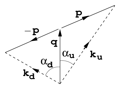
Figure 2.1: The momenta ${\mathbf{k}}_{u}$ and ${\mathbf{k}}_{d}$ of the two members of a LOFF-state Cooper pair. We choose the vector ${\mathbf{q}}$, common to all Cooper pairs, to coincide with the $z$-axis. The angles $\alpha_{u}({\mathbf{p}})$ and $\alpha_{d}({\mathbf{p}})$ indicate the polar angles of ${\mathbf{k}}_{u}$ and ${\mathbf{k}}_{d}$, respectively.

With this in mind, here is a suitable trial wavefunction for the LOFF state with wavevector ${\mathbf{q}}$ [65, 66, 89]:

$$\begin{array}[]{rcl}|\Psi_{{\mathbf{q}}}\rangle&=&B^{\dagger}_{L}B^{\dagger}_{R}|0\rangle,\\[4.30554pt] B^{\dagger}_{L}&=&\displaystyle\prod_{{\mathbf{p}}\in{\cal P},\alpha,\beta}\left(\cos\theta_{L}({\mathbf{p}})+\epsilon^{\alpha\beta 3}{\rm e}^{i\xi_{L}({\mathbf{p}})}\sin\theta_{L}({\mathbf{p}})\,a^{\dagger}_{Lu\alpha}({\mathbf{q}}\!+\!{\mathbf{p}})\,a^{\dagger}_{Ld\beta}({\mathbf{q}}\!-\!{\mathbf{p}})\right)\\[17.22217pt] &\times&\displaystyle\prod_{{\mathbf{p}}\in{\cal B}_{u},\alpha}a^{\dagger}_{Lu\alpha}({\mathbf{q}}\!+\!{\mathbf{p}})\times\displaystyle\prod_{{\mathbf{p}}\in{\cal B}_{d},\beta}a^{\dagger}_{Ld\beta}({\mathbf{q}}\!-\!{\mathbf{p}}),\\[12.91663pt] B^{\dagger}_{R}&=&\mbox{as above,~{}}L\to R,\end{array}$$ (2.2)

where $\alpha$, $\beta$ are color indices, $u$, $d$ and $L$, $R$ are the usual flavor and helicity labels, and $a^{\dagger}$ is the particle creation operator (for example, $a^{\dagger}_{Ld\alpha}$ creates a left-handed down quark with color $\alpha$). The $\theta$’s and $\xi$’s are the variational parameters of our ansatz: they are to be chosen to minimize the free energy of the LOFF state, as described in the next section. The first product in equation (2.2) creates quark pairs within a restricted region ${\cal P}$ of the total phase space. This allowed “pairing region” will be discussed below. The next product fills a “blocking region” ${\cal B}_{u}$ with unpaired up quarks: these are up quarks with momenta ${\mathbf{q}}+{\mathbf{p}}$ for which there are no corresponding down quarks with momenta ${\mathbf{q}}-{\mathbf{p}}$. The final product fills the blocking region ${\cal B}_{d}$ with unpaired down quarks. The ansatz does not contain a term that would create antiparticle pairs: we have checked the effect of such a term and found that it has no qualitative effect on our results.

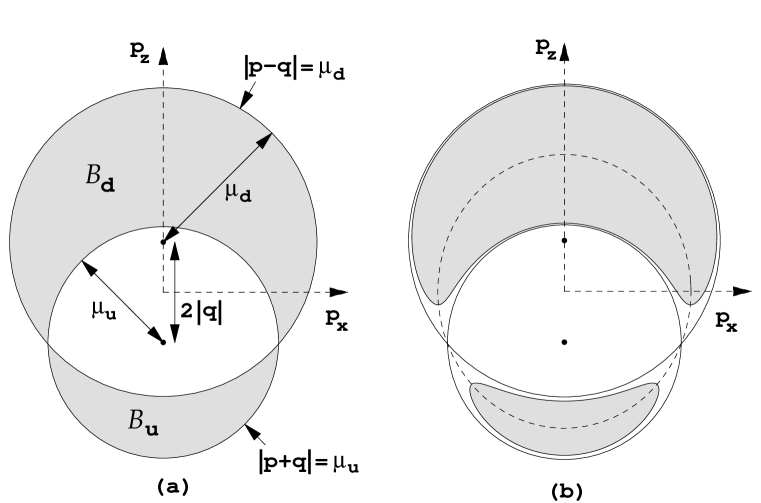
Figure 2.2: The LOFF phase space, as a function of ${\mathbf{p}}$ (Eq. (2.1)). We show the $p_{y}=0$ plane. (a) The phase space in the limit of arbitrarily weak interactions. In the shaded blocking regions ${\cal B}_{u}$ and ${\cal B}_{d}$, no pairing is possible. In the inner unshaded region, an interaction can induce hole-hole pairs. In the outer unshaded region, an interaction can induce particle-particle pairs. The region ${\cal P}$ (Eq. (2.2)) is the whole unshaded area. (b) When the effects of interactions and the formation of the LOFF state are taken into account, the blocking regions shrink. The BCS singularity occurs on the dashed ellipse, defined by $\epsilon_{u}+\epsilon_{d}=\mu_{u}+\mu_{d}$, where making a Cooper pair costs no free energy in the free case.

To complete the specification of our ansatz we need to describe the allowed pairing and blocking regions in phase space. These regions are largely determined by Pauli blocking as a result of populated Fermi seas. In the absence of pairing interactions, the system is in the “normal” state and up and down quarks are distributed in Fermi seas with Fermi momenta $p_{F}^{u}=\mu_{u}$ and $p_{F}^{d}=\mu_{d}$, respectively (recall that we consider massless quarks only, so the single particle energy of a quark with momentum ${\mathbf{k}}$ is $\epsilon({\mathbf{k}})=|{\mathbf{k}}|$). An up quark carries momentum ${\mathbf{k}}_{u}={\mathbf{p}}+{\mathbf{q}}$; in ${\mathbf{p}}$-space, therefore, the Fermi sea of up quarks corresponds to a sphere of radius $\mu_{u}={\bar{\mu}}-{\delta\mu}$ centered at $-{\mathbf{q}}$. Similarly, a down quark carries momentum ${\mathbf{k}}_{d}=-{\mathbf{p}}+{\mathbf{q}}$, giving a sphere in ${\mathbf{p}}$-space of radius $\mu_{d}={\bar{\mu}}+{\delta\mu}$ centered at $+{\mathbf{q}}$. The two offset spheres are shown in Figure 2.2a (we have drawn the case $|{\mathbf{q}}|>{\delta\mu}$ so that the two Fermi surfaces intersect in ${\mathbf{p}}$-space). In the limit of arbitrarily weak interactions, the blocking region ${\cal B}_{u}$ corresponds to the lower shaded area in the figure: pairing does not occur here since the region is inside the Fermi sea of up quarks, but outside the Fermi sea of down quarks. Similarly the upper shaded area is the blocking region ${\cal B}_{d}$. The entire unshaded area is the pairing region ${\cal P}$: it includes the region inside both spheres, where hole-hole pairing can occur, and the region outside both spheres, where particle-particle pairing can occur.

We can now explain how the LOFF wavefunction ansatz can describe the normal state with no condensate: we choose $\theta_{L}({\mathbf{p}})=\theta_{R}({\mathbf{p}})=\pi/2$ for ${\mathbf{p}}$ inside both Fermi spheres, and otherwise all the $\theta$’s are zero. With this choice the first term in Eq. (2.2) fills that part of each Fermi sea corresponding to the inner unshaded region of Figure 2.2a. The ${\cal B}_{u}$ and ${\cal B}_{d}$ terms fill out the remainder of each Fermi sea to obtain the normal state. Note that in the absence of pairing, the normal state can be described with any choice of ${\mathbf{q}}$. The most convenient choice is ${\mathbf{q}}=0$, in which case ${\mathbf{k}}_{u}={\mathbf{k}}_{d}={\mathbf{p}}$, ${\cal B}_{u}$ vanishes, and ${\cal B}_{d}$ is a spherical shell. Other choices of ${\mathbf{q}}$ correspond to choosing different origins of ${\mathbf{k}}_{u}$-space and ${\mathbf{k}}_{d}$-space, but in the absence of any interactions this has no consequence. Once we turn on interactions and allow pairing, we expect a particular $|{\mathbf{q}}|$ to be favored.

The phase space picture changes slightly when pairing interactions are included: the blocking regions are smaller when a LOFF condensate is present, as indicated in Figure 2.2b. We will account for this effect in the next section. With smaller blocking regions, a larger portion of the phase space becomes available for LOFF pairing. Such pairing is guaranteed to be energetically favorable when it costs zero free energy to create an up quark and a down quark, since these quarks can then pair to obtain a negative interaction energy. The zero free energy condition is

$$\epsilon({\mathbf{k}}_{u})+\epsilon({\mathbf{k}}_{d})=\mu_{u}+\mu_{d}=2\bar{\mu}$$ (2.3)

where $\epsilon({\mathbf{k}})$ is the single particle energy of a quark with momentum ${\mathbf{k}}$. For massless quarks, we obtain $|{\mathbf{q}}+{\mathbf{p}}|+|{\mathbf{q}}-{\mathbf{p}}|=2\bar{\mu}$, which describes an ellipsoidal surface in ${\mathbf{p}}$-space. This surface is indicated by the ellipse shown in Figure 2.2b; notice that the ellipsoid and the two Fermi surfaces all intersect at a circle.

If the interaction is weak, we expect LOFF pairing to be favored in a thin layer of phase space around this ellipsoid. This is manifest in the gap equation derived in the next section (Eq. (2.14)) in which, as in BCS theory, we find a divergent integrand on this ellipsoid in the absence of pairing. Pairing smooths the divergence. As the interaction gets stronger, the layer of favored pairing gets thicker. If there were no blocking regions, we could use the entire ellipsoid, just as BCS pairs condense over the entire spherical surface $|{\mathbf{p}}|=\mu$ in the symmetric, ${\delta\mu}=|{\mathbf{q}}|=0$ case. However, as shown in Figure 2.2b, the blocking regions exclude pairing over most of the ellipsoid, leaving a ribbon of unsuppressed LOFF pairing in the vicinity of the circle where the Fermi surfaces intersect. This agrees with our expectation for the particle distribution in the LOFF state: it is as in the normal state, except that there is a restricted region (around the aforementioned ribbon) where each quark in a pair can be near its Fermi surface and where pairing therefore occurs.

Although the constant single-particle energy contours for noninteracting up and down quarks cross in ${\mathbf{p}}$-space (see Figure 2.2a), we emphasize that the Fermi surfaces of up and down quarks do not cross in momentum (${\mathbf{k}}_{u}$- and ${\mathbf{k}}_{d}$-) space. The ${\mathbf{p}}$-space ribbon of unsuppressed pairing corresponds to unsuppressed pairing between up and down quarks with momenta around ${\mathbf{k}}$-space ribbons near their respective (disjoint) Fermi surfaces.

In the limit of arbitrarily weak interactions, the ribbon in momentum space along which pairing is unsuppressed shrinks, as the blocking regions grow to exclude all of the ellipsoid except the one-dimensional circle at which the two spheres in Figure 2.2 intersect. This circle has insufficient phase space to lead to a singularity in the gap equation: the integrand is singular on this circle, but the integral does not diverge. Therefore, the LOFF state is not guaranteed to occur if one takes the weak coupling limit at fixed ${\delta\mu}$. In this respect, the LOFF state is like the BCS state at nonzero ${\delta\mu}$: for weak coupling, $\Delta_{0}\rightarrow 0$ and because the BCS state can only exist if it has $\Delta_{0}>\sqrt{2}{\delta\mu}$, it must vanish for couplings weaker than some threshold. We shall see, however, that at any fixed weak coupling, the LOFF state, like the BCS state, is guaranteed to occur at some ${\delta\mu}$: the BCS state arises if ${\delta\mu}<{\delta\mu}_{1}$ and the LOFF state arises if ${\delta\mu}_{1}<{\delta\mu}<{\delta\mu}_{2}$.

One of the most striking features of the LOFF state is the spin structure of the condensate. The familiar “2SC” state pairs quarks of the same helicity and opposite momentum, so the spins are antiparallel and the quarks are arranged in an antisymmetric combination to form spin singlet Cooper pairs. The LOFF state also pairs quarks of the same helicity, but now the quark momenta are no longer antiparallel, as can be seen from Figure 2.1. Therefore the LOFF Cooper pairs cannot be spin singlets: they are superpositions of both spin zero and spin one. This is revealed explicitly by evaluating the nonzero $\langle\psi\psi\rangle$ expectation values in the LOFF state:

$$\begin{array}[]{rcl}-\langle\Psi_{{\mathbf{q}}}|\epsilon_{ij}\epsilon_{\alpha\beta 3}\,\psi^{i\alpha}({\mathbf{r}})CL\,\psi^{j\beta}({\mathbf{r}})|\Psi_{{\mathbf{q}}}\rangle&=&2\Gamma_{A}^{L}{\rm e}^{i2{\mathbf{q}}\cdot{\mathbf{r}}}\\[4.30554pt] i\langle\Psi_{{\mathbf{q}}}|(\sigma_{1})_{ij}\epsilon_{\alpha\beta 3}\,\psi^{i\alpha}({\mathbf{r}})CL\sigma^{03}\,\psi^{j\beta}({\mathbf{r}})|\Psi_{{\mathbf{q}}}\rangle&=&2\Gamma_{B}^{L}{\rm e}^{i2{\mathbf{q}}\cdot{\mathbf{r}}}\end{array}$$ (2.4)

where $i$, $j$ are flavor indices (1 = up, 2 = down), $\alpha$, $\beta$ are color indices, $C=i\gamma^{0}\gamma^{2}$, $L=(1-\gamma_{5})/2$ is the usual left-handed projection operator, and $\sigma_{\mu\nu}=(i/2)[\gamma_{\mu},\gamma_{\nu}]$. The constants $\Gamma_{A}^{L}$ and $\Gamma_{B}^{L}$ are left-handed $J=0$ and $J=1$ condensates, respectively. $\Gamma_{A}^{R}$ and $\Gamma_{B}^{R}$ are defined analogously. The $\Gamma$’s can be expressed in terms of the variational parameters of the LOFF wavefunction:

$$\begin{array}[]{rcl}\Gamma_{A}^{L}&=&\displaystyle\frac{4}{V}\displaystyle\sum_{{\mathbf{p}}\in{\cal P}}\sin\theta_{L}({\mathbf{p}})\cos\theta_{L}({\mathbf{p}}){\rm e}^{i\xi_{L}({\mathbf{p}})}\,\sin\Bigl{(}\frac{\alpha_{u}({\mathbf{p}})+\alpha_{d}({\mathbf{p}})}{2}\Bigr{)}{\rm e}^{-i\phi({\mathbf{p}})}\\[4.30554pt] \Gamma_{B}^{L}&=&\displaystyle\frac{4}{V}\displaystyle\sum_{{\mathbf{p}}\in{\cal P}}\sin\theta_{L}({\mathbf{p}})\cos\theta_{L}({\mathbf{p}}){\rm e}^{i\xi_{L}({\mathbf{p}})}\,\sin\Bigl{(}\frac{\alpha_{u}({\mathbf{p}})-\alpha_{d}({\mathbf{p}})}{2}\Bigr{)}{\rm e}^{-i\phi({\mathbf{p}})}\end{array}$$ (2.5)

Here $V$ is the spatial volume of the system, $\alpha({\mathbf{p}})$ are the polar angles of the quark momenta, as in Figure 2.1, and the dependence on the azimuthal angle $\phi$ follows from our use of the spinor conventions described in Refs.  [7, 9, 11]. The expressions for $\Gamma_{A}^{R}$ and $\Gamma_{B}^{R}$ are the same as those in (2.5) except that $\phi({\mathbf{p}})$ is replaced by $\pi-\phi({\mathbf{p}})$. In Eq. (2.5) and throughout, $(1/V)\sum_{\mathbf{p}}$ becomes $\int d^{3}p/(2\pi)^{3}$ in an infinite system.

Once we have derived a gap equation by minimizing the free energy with respect to these variational parameters, we expect the condensates to be simply related to gap parameters occurring in the gap equation. We will see explicitly how $\Gamma_{A}$ and $\Gamma_{B}$ are determined in the next section.

Notice that the condensates of Eq. (2.4) are plane waves in position space by virtue of the nonzero momentum $2{\mathbf{q}}$ of a Cooper pair. $\Gamma_{A}$ describes pairing which is antisymmetric in color, spin, and flavor, while $\Gamma_{B}$ describes pairing which is antisymmetric in color but symmetric in spin and flavor (in each case, Pauli statistics are obeyed). In the original LOFF condensate of electrons there can be no $\Gamma_{B}$, since electrons have no color or flavor, so that only the spin antisymmetric pairing is possible.

The $J=0$ condensates $\langle\psi CL\psi\rangle$, $\langle\psi CR\psi\rangle$ are Lorentz scalars (mixed under parity), while the $J=1$ condensates $\langle\psi CL\sigma^{03}\psi\rangle$, $\langle\psi CR\sigma^{03}\psi\rangle$ are 3-vectors (also mixed under parity) which point in the $z$-direction, parallel to the spontaneously chosen direction $\hat{\mathbf{q}}$ of the LOFF state. Because the ansatz contains a $J=1$ component, it would be interesting to generalize it to include the possibility of $LR$ pairing, in addition to $LL$ and $RR$ pairing. We discuss this further in Section 2.5.

2.3 The gap equation and free energy

Having presented a trial wavefunction for the LOFF state, we now proceed to minimize the expectation value of the free energy $\langle F\rangle$ with respect to the variational parameters of the wavefunction (the $\theta$’s and $\xi$’s of equation (2.2)) to obtain a LOFF gap equation. The free energy is $F=H-\mu_{u}N_{u}-\mu_{d}N_{d}$, where $H$ is the Hamiltonian, and $N_{u}$ and $N_{d}$ are the number operators for up and down quarks, respectively. We choose a model Hamiltonian which has a free quark term $H_{0}$ and an interaction term $H_{I}$, and write the free energy as $F=F_{0}+H_{I}$, where $F_{0}=H_{0}-\mu_{u}N_{u}-\mu_{d}N_{d}$ is the free energy for noninteracting quarks. To describe the pairing interaction between quarks, we use an NJL model consisting of a four-fermion interaction with the color and flavor structure of one-gluon exchange:

$$H_{I}=\frac{3}{8}\int d^{3}x\left[G_{E}(\bar{\psi}\gamma^{0}T^{A}\psi)(\bar{\psi}\gamma^{0}T^{A}\psi)-G_{M}(\bar{\psi}\gamma^{i}T^{A}\psi)(\bar{\psi}\gamma^{i}T^{A}\psi)\right]$$ (2.6)

where the $T^{A}$ are the color $SU(3)$ generators, normalized so that $\hbox{tr}(T^{A}T^{B})=2\delta^{AB}$. Notice that we have relaxed some constraints on the spin structure of one-gluon exchange: we allow for the possibility of independent couplings $G_{E}$ and $G_{M}$ for electric and magnetic gluons, respectively. This spoils Lorentz boost invariance but there is no reason to insist on boost invariance in a finite-density system. Indeed, in high density quark matter we expect screening of electric gluons but only Landau damping of magnetic gluons, and we might choose to model these effects by setting $G_{E}\ll G_{M}$. We postpone a discussion of these issues and their implications for the LOFF state until Section 2.5. For now, we restrict ourselves to the case of Lorentz invariant single gluon exchange, by letting $G_{E}=G_{M}=G>0$.

We need to evaluate the expectation value of $F$ in the LOFF state to obtain an expression for the free energy of the system in terms of the variational parameters of the ansatz. The noninteracting part of the free energy is simply

$$\begin{array}[]{rcl}\langle F_{0}\rangle&=&\displaystyle\sum_{{\mathbf{p}}\in{\cal B}_{u}}2(|{\mathbf{q}}+{\mathbf{p}}|-\mu_{u})+\sum_{{\mathbf{p}}\in{\cal B}_{d}}2(|{\mathbf{q}}-{\mathbf{p}}|-\mu_{d})\\ &&+\displaystyle\sum_{{\mathbf{p}}\in{\cal P}}2(|{\mathbf{q}}+{\mathbf{p}}|+|{\mathbf{q}}-{\mathbf{p}}|-\mu_{u}-\mu_{d})\sin^{2}\theta_{L}({\mathbf{p}})\\ &&+(\mbox{same, with }L\to R).\end{array}$$ (2.7)

The first and second terms represent the contributions of the unpaired left-handed up and down quarks, respectively. The third term gives the (noninteracting) free energy of the left-handed quark pairs. The three terms are all repeated with $L$ replaced by $R$ to include the free energy for the right-handed quarks. The factors of two in equation (2.7) appear because there are two quark colors (“red” and “green”) involved in the the condensate. The “blue” quarks do not participate in the pairing interaction and instead behave as free particles: the blue up and down quarks fill Fermi seas with Fermi momenta $p_{F}^{u}=\mu_{u}$ and $p_{F}^{d}=\mu_{d}$, respectively. Below, we will want to compare the free energy of the LOFF, BCS and normal states. Since at any given $\mu_{u}$ and $\mu_{d}$ the free energy of the spectator quarks is the same in all three states, we can neglect these blue quarks in the remainder of our analysis even though they do contribute to the total free energy.

The expectation value of $H_{I}$ gives the total binding energy of the pairing interaction:

$$\langle H_{I}\rangle=-{\textstyle\frac{1}{2}}GV\left(|\Gamma^{L}_{A}|^{2}+|\Gamma^{R}_{A}|^{2}\right)$$ (2.8)

where the $\Gamma_{A}$’s are the $J=0$ LOFF condensates defined in equations (2.5). These condensates are simply related to $J=0$ LOFF gap parameters defined as

$$\Delta^{\{L,R\}}_{A}=G\Gamma_{A}^{\{L,R\}}\ .$$ (2.9)

The gap parameters $\Delta_{A}$ correspond to 1PI Green’s functions and are the quantities which will appear in the quasiparticle dispersion relations and for which we will derive the self-consistency conditions conventionally called gap equations. We see from Eq. (2.8) that with $G>0$ the interaction is attractive in the $J=0$ channel and is neither attractive nor repulsive in the $J=1$ channel.

Our ansatz breaks rotational invariance, so once $J=0$ pairing occurs ($\Gamma_{A}\neq 0$) we expect that there will also be $J=1$ pairing ($\Gamma_{B}\neq 0$). As we have seen, this arises even in the absence of any interaction in the $J=1$ channel as a consequence of the fact that the momenta of two quarks in a Cooper pair are not anti-parallel if ${\mathbf{q}}\neq 0$. Because $\langle H\rangle$ is independent of $\Gamma_{B}$, the quasiparticle dispersion relations must also be independent of $\Gamma_{B}$. That is, the $J=1$ gap parameter must vanish: $\Delta_{B}=0$. In Section 2.5, we shall see by direct calculation that $\Delta_{B}$ is proportional to $(G_{E}-G_{M})\Gamma_{B}$. In the present analysis with $G_{E}=G_{M}$, therefore, $\Delta_{B}=0$ while $\Gamma_{B}\neq 0$.

The $\xi$’s are chosen to cancel the azimuthal phases $\phi({\mathbf{p}})$ in equations (2.5). By this choice we obtain maximum coherence in the sums over ${\mathbf{p}}$, giving the largest possible magnitudes for the condensates and gap parameters. We have

$$\xi_{L}({\mathbf{p}})=\phi({\mathbf{p}})+\varphi_{L},\hskip 21.68121pt\xi_{R}({\mathbf{p}})=\pi-\phi({\mathbf{p}})+\varphi_{R}$$ (2.10)

where $\varphi_{L}$ and $\varphi_{R}$ are arbitrary ${\mathbf{p}}$-independent angles. These constant phases do not affect the free energy — they correspond to the Goldstone bosons for the broken left-handed and right-handed baryon number symmetries — and are therefore not constrained by the variational procedure. For convenience, we set $\varphi_{L}=\varphi_{R}=0$ and obtain condensates and gap parameters that are purely real.

The relative phase $\varphi_{L}-\varphi_{R}$ determines how the LOFF condensate transforms under a parity transformation. Its value determines whether the $J=0$ condensate is scalar, pseudoscalar, or an arbitrary combination of the two and whether the $J=1$ condensate is vector, pseudovector, or an arbitrary combination. Because single gluon exchange cannot change the handedness of a massless quark, the left- and right-handed condensates in the LOFF phase are not coupled in the free energy of Eq. (2.8.) Our choice of interaction Hamiltonian therefore allows an arbitrary choice of $\varphi_{L}-\varphi_{R}$. A global $U(1)_{A}$ transformation changes $\varphi_{L}-\varphi_{R}$, and indeed this is a symmetry of our toy model. If we included $U(1)_{A}$-breaking interactions in our Hamiltonian, to obtain a more complete description of QCD, we would find that the free energy depends on $\varphi_{L}-\varphi_{R}$, and thus selects a preferred value. For example, had we taken $H_{I}$ to be the two-flavor instanton interaction as in Ref. [9, 10], the interaction energy would appear as $\Gamma^{L*}\Gamma^{R}+\Gamma^{L}\Gamma^{R*}$ instead of as in (2.8). This would enforce a fixed phase relation $\varphi_{L}-\varphi_{R}=0$, favoring condensates which are parity conserving [9, 10].

We now apply the variational method to determine the angles $\theta({\mathbf{p}})$ in our trial wavefunction, by requiring that the free energy is minimized: $\partial\langle F\rangle/\partial\theta({\mathbf{p}})=0$. This is complicated by the fact that the pairing region ${\cal P}$ and the blocking regions ${\cal B}_{u}$ and ${\cal B}_{d}$ are themselves implicitly dependent on the $\theta$ angles: these angles determine the extent of the LOFF pairing, and the phase space regions ${\cal P}$, ${\cal B}_{u}$ and ${\cal B}_{d}$ change when a condensate is present, as mentioned in Section 2.2. For now we simply ignore any $\theta$-dependence of the phase space regions; our result will nevertheless turn out to be correct. Everything is the same for left and right condensates so we hereafter drop the $L$ and $R$ labels. Upon variation with respect to $\theta({\mathbf{p}})$, we obtain

$$\tan 2\theta({\mathbf{p}})=\frac{2\Delta_{A}\sin(\beta_{A}({\mathbf{p}})/2)}{|{\mathbf{q}}+{\mathbf{p}}|+|{\mathbf{q}}-{\mathbf{p}}|-\mu_{u}-\mu_{d}}$$ (2.11)

where $\beta_{A}({\mathbf{p}})=\alpha_{u}({\mathbf{p}})+\alpha_{d}({\mathbf{p}})$ is the angle between the two quark momenta in a LOFF pair, as shown in Figure 2.1. Notice that the denominator on the right hand side of the above expression vanishes along the ellipsoidal surface of optimal LOFF pairing described in Section 2.2. When ${\mathbf{q}}=0$, the quark momenta are antiparallel so $\beta_{A}({\mathbf{p}})=\pi$ and Eq. (2.11) reduces to the simple BCS result: $\tan 2\theta=\Delta_{A}/(|{\mathbf{p}}|-{\bar{\mu}})$.

With the $\theta$ angles now expressed in terms of a gap parameter $\Delta_{A}$, we turn to the LOFF quasiparticle dispersion relations. They can be obtained by taking the absolute value of the expressions

$$\begin{array}[]{rcrcl}E_{1}({\mathbf{p}})&=&{\delta\mu}&+&{\textstyle\frac{1}{2}}(|{\mathbf{q}}+{\mathbf{p}}|-|{\mathbf{q}}-{\mathbf{p}}|)\\[4.30554pt] &&&+&{\textstyle\frac{1}{2}}\sqrt{(|{\mathbf{q}}+{\mathbf{p}}|+|{\mathbf{q}}-{\mathbf{p}}|-2\bar{\mu})^{2}+4\Delta_{A}^{2}\sin^{2}({\textstyle\frac{1}{2}}\beta_{A}({\mathbf{p}}))}\\[8.61108pt] E_{2}({\mathbf{p}})&=&-{\delta\mu}&-&{\textstyle\frac{1}{2}}(|{\mathbf{q}}+{\mathbf{p}}|-|{\mathbf{q}}-{\mathbf{p}}|)\\[4.30554pt] &&&+&{\textstyle\frac{1}{2}}\sqrt{(|{\mathbf{q}}+{\mathbf{p}}|+|{\mathbf{q}}-{\mathbf{p}}|-2\bar{\mu})^{2}+4\Delta_{A}^{2}\sin^{2}({\textstyle\frac{1}{2}}\beta_{A}({\mathbf{p}}))}\ ,\\ \end{array}$$ (2.12)

whose meaning we now describe. For regions of ${\mathbf{p}}$-space which are well outside both Fermi surfaces, $E_{1}$ ($E_{2}$) is the free energy cost of removing a LOFF pair and adding an up quark with momentum ${\mathbf{q}}+{\mathbf{p}}$ (a down quark with momentum ${\mathbf{q}}-{\mathbf{p}}$). For regions of ${\mathbf{p}}$-space which are well inside both Fermi surfaces, $E_{1}$ ($E_{2}$) is the free energy cost of removing a LOFF hole pair and adding a down hole with momentum ${\mathbf{q}}-{\mathbf{p}}$ (an up hole with momentum ${\mathbf{q}}+{\mathbf{p}}$). Where the Fermi surfaces cross in ${\mathbf{p}}$-space and pairing is maximal, both quasiparticles are equal superpositions of up and down. In the region of ${\mathbf{p}}$-space which is well inside the up Fermi surface but well outside the down Fermi surface, $E_{1}$ is negative, corresponding to a domain in which it is energetically favorable to have an unpaired up quark with momentum ${\mathbf{q}}+{\mathbf{p}}$ rather than a $({\mathbf{q}}+{\mathbf{p}},{\mathbf{q}}-{\mathbf{p}})$ quark pair. Similarly, $E_{2}$ is negative where it is favorable to have an unpaired down quark with momentum ${\mathbf{q}}-{\mathbf{p}}$ rather than a LOFF pair. Equations (2.12) allow us to finally complete our description of the LOFF phase by specifying the definitions of the phase space regions ${\cal P}$, ${\cal B}_{u}$ and ${\cal B}_{d}$. The blocking region ${\cal B}_{u}$ is the region where $E_{1}({\mathbf{p}})$ is negative, and unpaired up quarks are favored over LOFF pairs. Similarly ${\cal B}_{d}$ is the region where $E_{2}({\mathbf{p}})$ is negative. The regions $E_{1}<0$ and $E_{2}<0$ are shown as the shaded areas in Figure 2.2a for $\Delta_{A}=0$, and in Figure 2.2b for $\Delta_{A}\neq 0$. LOFF pairing occurs in the region where $E_{1}$ and $E_{2}$ are both positive:

$${\cal P}=\{{\mathbf{p}}|E_{1}({\mathbf{p}})>0\mbox{ and }E_{2}({\mathbf{p}})>0\}$$ (2.13)

corresponding to the entire unshaded regions of Figure 2.2. The actual quasiparticle dispersion functions are $|E_{1}({\mathbf{p}})|$ and $|E_{2}({\mathbf{p}})|$: they are nonnegative everywhere, since they represent energies of perturbations of the LOFF state which is the presumed ground state of the system. In the blocking regions, elementary excitations are created by replacing an unpaired quark with a quark pair, and vice versa in the pairing region. When ${\mathbf{q}}=0$, Eqs. (2.12) reduce to the more familiar BCS result: $E_{\{1,2\}}({\mathbf{p}})=\pm{\delta\mu}+\sqrt{(|{\mathbf{p}}|-\bar{\mu})^{2}+\Delta_{A}^{2}}$.

With the boundaries of the blocking regions specified, one can verify by explicit calculation that the variation of these boundaries upon variation of the $\theta$’s does not change the free energy. This can be understood as follows. Notice that because we can create zero-energy quasiparticles on the boundaries of the blocking regions, there is no actual energy gap in the excitation spectrum of the LOFF state. The change in $\langle F\rangle$ due to variation of the boundaries of the blocking regions is zero because this variation simply creates zero-free-energy quasiparticles on these boundaries. This justifies our neglect of the $\theta$-dependence of the phase space regions in the derivation of Eq. (2.11).

Substituting the expression (2.11) for the $\theta$ angles into the expression (2.5) for the $\Gamma_{A}$ condensate, and using the relation $\Delta_{A}=G\Gamma_{A}$, we obtain a self-consistency equation for the gap parameter $\Delta_{A}$:

$$1=\frac{2G}{V}\sum_{{\mathbf{p}}\in{\cal P}}\frac{2\sin^{2}({\textstyle\frac{1}{2}}\beta_{A}({\mathbf{p}}))}{\sqrt{(|{\mathbf{q}}+{\mathbf{p}}|+|{\mathbf{q}}-{\mathbf{p}}|-2\bar{\mu})^{2}+4\Delta_{A}^{2}\sin^{2}({\textstyle\frac{1}{2}}\beta_{A}({\mathbf{p}}))}}.$$ (2.14)

This can be compared to the BCS gap equation, obtained upon setting ${\mathbf{q}}=0$ and eliminating the blocking regions:

$$1=\frac{2G}{V}\sum_{\mathbf{p}}\frac{1}{\sqrt{(|{\mathbf{p}}|-\bar{\mu})^{2}+\Delta_{0}^{2}}}\ .$$ (2.15)

Note that in the LOFF gap equation (2.14), the gap parameter appears on the right hand side both explicitly in the denominator and also implicitly in the definition of the pairing region ${\cal P}$, as given in (2.13). This means that if the ${\mathbf{q}}\rightarrow 0$ limit is taken at fixed ${\delta\mu}$, the LOFF gap equation will only become the BCS gap equation if the blocking regions vanish in this limit. This happens if, as ${\mathbf{q}}\rightarrow 0$, $\Delta_{A}$ tends to a limiting value which is greater than ${\delta\mu}$. For $\Delta_{A}<{\delta\mu}$, the blocking region $\mathcal{B}_{d}$ does not disappear but instead becomes a spherical shell, as we can see by taking ${\mathbf{q}}\rightarrow 0$ in figure 2.2. Pairing is blocked in the region

$$\bar{\mu}-\sqrt{{\delta\mu}^{2}-\Delta_{A}^{2}}<|{\mathbf{p}}|<\bar{\mu}+\sqrt{{\delta\mu}^{2}-\Delta_{A}^{2}}.$$ (2.16)

This is precisely the “breached pair” color superconductor discussed in chapter 1 [75, 76]; the breach is just the blocking region $\mathcal{B}_{d}$. This second solution to the ${\mathbf{q}}=0$ gap equation was first discovered by Sarma [74]. In the present calculation such states will always have higher free energy than both the unpaired state ($\Delta_{A}=0$) and the BCS state obtained by solving the gap equation (2.15) with no blocking regions.. But there may exist other scenarios in which the Sarma solution is favored: when one species is very heavy and the other very light, for example [76].

In the next section we will solve the LOFF gap equation (2.14) and determine the circumstances in which the LOFF state is the true ground state of the system. Once we have obtained a solution to the gap equation (2.14) for $\Delta_{A}$, the condensates are given by $\Gamma_{A}=\Delta_{A}/G$ and

$$\Gamma_{B}=\displaystyle\frac{2}{V}\sum_{{\mathbf{p}}\in{\cal P}}\frac{2\Delta_{A}\sin({\textstyle\frac{1}{2}}\beta_{A}({\mathbf{p}}))\sin({\textstyle\frac{1}{2}}\beta_{B}({\mathbf{p}}))}{\sqrt{(|{\mathbf{q}}+{\mathbf{p}}|+|{\mathbf{q}}-{\mathbf{p}}|-2\bar{\mu})^{2}+4\Delta_{A}^{2}\sin^{2}({\textstyle\frac{1}{2}}\beta_{A}({\mathbf{p}}))}}$$ (2.17)

where $\beta_{B}({\mathbf{p}})=\alpha_{u}({\mathbf{p}})-\alpha_{d}({\mathbf{p}})$. (See Figure 2.1.) We now see explicitly that if the interaction is attractive in the $J=0$ channel, creating a nonzero $\Gamma_{A}$ and $\Delta_{A}$, a nonzero $J=1$ condensate $\Gamma_{B}$ is induced regardless of the fact that there is no interaction in the $J=1$ channel. As a check, note that if ${\mathbf{q}}=0$, $\sin({\textstyle\frac{1}{2}}\beta_{A}({\mathbf{p}}))=1$ and $\sin({\textstyle\frac{1}{2}}\beta_{B}({\mathbf{p}}))$ is given by the cosine of the polar angle of ${\mathbf{p}}$. The right hand side of (2.17) therefore vanishes upon integration, and $\Gamma_{B}$ vanishes when ${\mathbf{q}}=0$ as it should. It is now apparent that two features contribute to a nonzero $\Gamma_{B}$. The first is that the momenta in a quark pair are not antiparallel, which leads to the factors of $\sin({\textstyle\frac{1}{2}}\beta_{A}({\mathbf{p}}))$ in Eq. (2.17). The second is that the pairing region is anisotropic, since if it were not the factor of $\sin({\textstyle\frac{1}{2}}\beta_{B}({\mathbf{p}}))$ would ensure that the right-hand side of (2.17) vanishes upon integration.

As written, the gap equations (2.14) and (2.15) are ultraviolet divergent. In QCD, of course, asymptotic freedom implies that the interaction between quarks decreases at large momentum transfer and we have not yet represented this fact in our toy model. In previous work [9, 11, 23], we chose to mimic the effects of asymptotic freedom (and to render the right hand side of the gap equation finite) by introducing a form factor associated with each fermion leg in the four-fermion interaction. This is not a good strategy when ${\mathbf{q}}\neq 0$. The two incident quarks carry momenta ${\mathbf{q}}+{\mathbf{p}}$ and ${\mathbf{q}}-{\mathbf{p}}$ while the outgoing quarks carry momenta ${\mathbf{q}}+{\mathbf{p}}^{\prime}$ and ${\mathbf{q}}-{\mathbf{p}}^{\prime}$. Were we to cut off these four momenta with form factors on each leg, we would have a cutoff which depends explicitly on ${\mathbf{q}}$. This is not a good representation of what happens in full QCD, in which the condition for when the interaction becomes weak is determined by the momentum ${\mathbf{p}}-{\mathbf{p}}^{\prime}$ transferred through the gluon and has nothing to do with ${\mathbf{q}}$. For simplicity, we choose to introduce a hard cutoff in our NJL model, rather than a smooth form factor, and choose simply to cut off the momentum ${\mathbf{p}}$. This is not equivalent to cutting off the momentum transfer, but has the desired feature of being a ${\mathbf{q}}$-independent cutoff. That is, we limit the integration region to $|{\mathbf{p}}|<\Lambda$ in the BCS gap equation (2.15) and to $\{{\mathbf{p}}\in{\cal P}$ and $|{\mathbf{p}}|<\Lambda\}$ in the LOFF gap equation (2.14). In the BCS case, this criterion is equivalent to cutting off the momentum of each fermion leg. In the LOFF case, it is not equivalent and is more appropriate. The choice we have made is not the only ${\mathbf{q}}$-independent cutoff one might try. For example, we have also obtained results upon cutting off momenta outside a large ellipsoid in ${\mathbf{p}}$-space, confocal with the centers of the two Fermi spheres in Figure 2.2, but have found that this makes little difference relative to the simpler choice of the large sphere $|{\mathbf{p}}|<\Lambda$.

2.4 Results

We solve the gap equation (2.14) numerically (and analytically in the limit $\Delta_{A}\ll{\delta\mu},q,\Delta_{0}$) and calculate the LOFF state free energy as a function of ${\delta\mu}$ and $q$, for given coupling $G$, average chemical potential ${\bar{\mu}}$, and cutoff $\Lambda$. We vary $q$ to minimize the LOFF free energy, and compare it with that for the standard BCS pairing (2.15) to see which is favored. In this way we can map out the phase diagram for the three phases of pairing between the two species of quark: BCS, LOFF, and unpaired.

Note that the solution to the gap equation, the LOFF gap parameter $\Delta_{A}$, is not a gap in the spectrum of excitations. The quasiparticle dispersion relations (2.12) vary with the direction of the momentum, yielding gaps that vary from zero (for momenta on the edge of the blocking regions in phase space) up to a maximum of $\Delta_{A}$.

We will first discuss the range of ${\delta\mu}$ in which there exists a LOFF state as a local energy minimum. Later we will go on to study the competition between LOFF and BCS, and see in what range of ${\delta\mu}$ the LOFF state is the global minimum. We expect the BCS state to be preferred when the mismatch ${\delta\mu}$ between the Fermi energies of the two species is small. When the mismatch is comparable to the BCS gap (${\delta\mu}\sim\Delta_{0}$) we expect a transition to LOFF, and at larger ${\delta\mu}$ we expect all pairing to cease. These expectations are largely borne out.

In general we fix $\Lambda=1~{}{\rm GeV}$ and ${\bar{\mu}}=0.4~{}{\rm GeV}$, and study different coupling strengths $G$ which we parameterize by the physical quantity $\Delta_{0}$, the BCS gap of Eq. (2.15) which increases monotonically with increasing $G$. When we wish to study the dependence on the cutoff, we vary $\Lambda$ while at the same time varying the coupling $G$ such that $\Delta_{0}$ is kept fixed. (This is in the same spirit as using a renormalization condition on a physical quantity—$\Delta_{0}$—to fix the “bare” coupling—$G$.) We expect that the relation between other physical quantities and $\Delta_{0}$ will be reasonably insensitive to variation of the cutoff $\Lambda$.

XX

Figure 2.3: (a) The zero-gap curves for the LOFF state. To the right of a solid curve, there is no solution to the LOFF gap equation, to the left of the curve there is a solution, and on the curve the gap parameter is zero. The three curves are (from strongest to weakest coupling): $\Delta_{0}=0.1,0.04,0.01~{}{\rm GeV}$. The region $q<{\delta\mu}$ is complicated to describe [66], and solutions found in this region never give the lowest free energy state at a given ${\delta\mu}$. (b) Here, we choose $\Delta_{0}=0.04~{}{\rm GeV}$ and focus on the region near ${\delta\mu_{2}}$, the maximum value of ${\delta\mu}$ at which the LOFF state exists. The dashed curve shows the value of $|{\mathbf{q}}|$ which minimizes the free energy of the LOFF state at a given ${\delta\mu}$. ${\delta\mu_{1}}$, discussed below, is also indicated.

We wish to determine ${\delta\mu}_{2}$, the boundary separating the LOFF phase and the normal phase. The LOFF to unpaired phase transition is second order, so it occurs where the solution $\Delta_{A}$ to the LOFF gap equation (2.14) is zero. Setting $\Delta_{A}=0$ in the gap equation (2.15) yields an analytical expression relating ${\delta\mu}$ and $q$, for any given $G$ and $\Lambda$. In Figure 2.3a we show the $\Delta_{A}=0$ curve for three couplings corresponding to $\Delta_{0}=0.1~{}{\rm GeV}$ (strong coupling), $\Delta_{0}=0.04~{}{\rm GeV}$ and $\Delta_{0}=0.01~{}{\rm GeV}$ (weak coupling). We have only drawn the zero-gap curve in the region where $q\geq{\delta\mu}$. We expect this to be the region of interest for LOFF pairing because when $q\geq{\delta\mu}$ the two spheres of Figure 2.2 do in fact intersect. We have verified that, as described in some detail in Ref. [66], there are regions of Figure 2.3a with $q<{\delta\mu}$ within which the LOFF gap equation (2.14) has (one or even two) nonzero solutions, but these solutions all correspond to phases whose free energy is either greater than that of the normal phase or greater than that of the BCS phase or both. Figure 2.3 shows that for a given coupling strength, parameterized by $\Delta_{0}$, there is a maximum ${\delta\mu}$ for which the LOFF state exists: we call it ${\delta\mu_{2}}$. For ${\delta\mu}>{\delta\mu_{2}}$, the mismatch of chemical potentials is too great for the LOFF phase to exist.

We see from Figure 2.3a that as the coupling gets weaker, ${\delta\mu_{2}}/\Delta_{0}$ gets gradually larger. (Of course, ${\delta\mu_{2}}$ itself gets smaller: the quantities plotted are ${\delta\mu}/\Delta_{0}$ and $q/\Delta_{0}$.) Note that in the $\Delta_{0}\rightarrow 0$ limit, the zero gap curve is essentially that shown in the figure for $\Delta_{0}=0.01~{}{\rm GeV}$, in agreement with the curve obtained at weak coupling by Fulde and Ferrell [66]. The fact that this curve ceases to move in the $\Delta_{0}\rightarrow 0$ limit means that ${\delta\mu_{2}}\rightarrow 0$ while ${\delta\mu_{2}}/\Delta_{0}\rightarrow{\rm const}$ in this limit.

For ${\delta\mu}\rightarrow{\delta\mu_{2}}$ from below, we see from Figure 2.3 that there is a solution to the LOFF gap equation only at a single value of $q$. For example, at $\Delta_{0}=0.04~{}{\rm GeV}$ we find $q=0.880\Delta_{0}=1.183\,{\delta\mu_{2}}$ at ${\delta\mu_{2}}=0.744\Delta_{0}$. (In agreement with Refs. [65, 66], in the weak coupling limit we find $q=0.906\Delta_{0}=1.20\,{\delta\mu_{2}}$ at ${\delta\mu_{2}}=0.754\Delta_{0}$.) For any value of ${\delta\mu}<{\delta\mu_{2}}$, solutions to the LOFF gap equation exist for a range of $|{\mathbf{q}}|$. We must now find the value of $|{\mathbf{q}}|$ for which the free energy of the LOFF state is minimized. We obtain the free energy of the LOFF state at a point in Figure 2.3 by first solving the gap equation (2.14) numerically to obtain $\Delta_{A}$, and then using (2.9) and (2.11) to evaluate $\langle F_{0}+H_{I}\rangle$ given in (2.7) and (2.8). For each value of ${\delta\mu}<{\delta\mu_{2}}$ we can now determine which choice of $q$ yields the lowest free energy. The resulting “best-$q$ curve” curve is shown in Figure 2.3b for $\Delta_{0}=0.04~{}{\rm GeV}$.

Figure 2.4: LOFF and BCS gaps and free energies as a function of ${\delta\mu}$, with coupling chosen so that $\Delta_{0}=40{\rm~{}MeV}$ and with ${\bar{\mu}}=0.4~{}{\rm GeV},\Lambda=1~{}{\rm GeV}$. Free energies are measured relative to the normal state. At each ${\delta\mu}$ we have varied $q$ to find the best LOFF state. The vertical dashed line marks ${\delta\mu}={\delta\mu}_{1}$, the value of ${\delta\mu}$ above which the LOFF state has lower free energy than BCS. The expanded inset (wherein $s=10^{-7}~{}{\rm GeV}^{4}$) focuses on the region ${\delta\mu}_{1}<{\delta\mu}<{\delta\mu}_{2}$ where the LOFF state has the lowest free energy. This figure should be compared with the sketch in figure 1.4.

Finally, for each point on the best-$q$ curve we ask whether the LOFF free energy at that ${\delta\mu}$ and (best) $q$ is more or less than the free energy of the BCS state at the same ${\delta\mu}$. In this way, we find ${\delta\mu_{1}}$ at which a first order phase transition between the LOFF and BCS states occurs. In Figure 2.4 we show the competition between the BCS and LOFF states as a function of the Fermi surface mismatch ${\delta\mu}$, for a fixed coupling corresponding to $\Delta_{0}=40$ MeV. The LOFF state exists for ${\delta\mu}<{\delta\mu_{2}}=0.744\Delta_{0}$. At each ${\delta\mu}<{\delta\mu_{2}}$, we plot the gap parameter and free energy characterizing the LOFF state with the best $q$ for that ${\delta\mu}$. Although the BCS gap $\Delta_{0}$ is larger than the LOFF gap $\Delta_{A}$, as ${\delta\mu}$ increases we see from Eq. (1.16) that the BCS state pays a steadily increasing free-energetic price for maintaining $p_{F}^{u}=p_{F}^{d}$, whereas the LOFF state pays no such price. We now see that the LOFF state has lower free energy than the BCS state for ${\delta\mu}>{\delta\mu_{1}}$, in this case ${\delta\mu_{1}}=0.7104\Delta_{0}$. At ${\delta\mu}={\delta\mu_{1}}$, the gap parameter is $\Delta_{A}=0.0078~{}{\rm GeV}=0.195\Delta_{0}$. (Had we calculated ${\delta\mu}_{1}$ by comparing the BCS free energy with that of the unpaired state instead of with that of the LOFF state, we would have obtained ${\delta\mu_{1}}=0.711\Delta_{0}$. As the inset to Figure 2.4 confirms, the BCS free energy varies so rapidly that this makes an almost imperceptible difference. In later figures, we therefore obtain ${\delta\mu_{1}}$ via the simpler route of comparing BCS vs. normal.) At the coupling corresponding to $\Delta_{0}=40$ MeV, we have found that the LOFF state is favored over both the BCS state and the normal state in a “LOFF window” $0.710<{\delta\mu}/\Delta_{0}<0.744$.

Figure 2.5: The two LOFF condensates $\Gamma_{A}$ $(J=0)$ and $\Gamma_{B}$ $(J=1)$ for the same choice of parameters as in Figure 2.4. We focus on the region ${\delta\mu_{1}}<{\delta\mu}<{\delta\mu_{2}}$. For reference, in the BCS phase $\Gamma_{A}=\Delta_{0}/G=0.00583~{}{\rm GeV}^{3}$ and $\Gamma_{B}=0$.

With solutions to the gap equation in hand, we can obtain the $J=0$ condensate $\Gamma_{A}=G\Delta_{A}$ and the $J=1$ condensate $\Gamma_{B}$ given in Eq. (2.17). In Figure 2.5, we show both condensates within the LOFF window ${\delta\mu_{1}}<{\delta\mu}<{\delta\mu_{2}}$. We see first of all that $\Gamma_{B}\neq 0$, as advertised. For the choice of parameters in Figs. 2.4 and 2.5 we find $\Gamma_{B}/\Gamma_{A}$ essentially constant over the whole LOFF window, varying from 0.121 at ${\delta\mu_{1}}$ to 0.133 at ${\delta\mu_{2}}$. Increasing $\Delta_{0}$ tends to increase $\Gamma_{B}/\Gamma_{A}$, as does decreasing $\Lambda$. Second of all, we see that the phase transition at ${\delta\mu}={\delta\mu_{2}}$, between the LOFF and normal phases, is second order in the mean-field approximation we employ throughout.

Figure 2.6: The interval of ${\delta\mu}$ within which the LOFF state occurs, as a function of the coupling (parameterized as usual by the BCS gap $\Delta_{0}$). Below the solid line, there is a LOFF state. Below the dashed line, the BCS state is favored. The different lines of each type correspond to different cutoffs $\Lambda=0.8~{}{\rm GeV}$ to $1.6~{}{\rm GeV}$. ${\delta\mu_{1}}/\Delta_{0}$ and ${\delta\mu_{2}}/\Delta_{0}$ show little cutoff-dependence, and the cutoff-dependence disappears completely as $\Delta_{0},{\delta\mu}\to 0$.

It is interesting to explore how the width of the LOFF window depends on the strength of the coupling, and to confirm that it is insensitive to the cutoff. We do this in Figure 2.6, where we plot ${\delta\mu_{2}}/\Delta_{0}$ (solid lines) and ${\delta\mu_{1}}/\Delta_{0}$ (dashed lines). The LOFF state is favored for ${\delta\mu_{1}}/\Delta_{0}<{\delta\mu}/\Delta_{0}<{\delta\mu_{2}}/\Delta_{0}$, i.e. between the solid and dashed curves in Figure 2.6. In the weak coupling limit, the LOFF window tends to $0.707<{\delta\mu}/\Delta_{0}<0.754$ and $\Delta_{A}$ at ${\delta\mu_{1}}$ tends to $0.23\Delta_{0}$, as in Refs. [65, 66]. Note that if one takes the weak-coupling limit $\Delta_{0}\rightarrow 0$ at fixed ${\delta\mu}$, neither BCS nor LOFF pairing survives because ${\delta\mu}/\Delta_{0}\rightarrow\infty$. However, for any arbitrarily small but nonzero coupling, the LOFF phase is favored within a range of ${\delta\mu}$. Figure 2.6 thus demonstrates that in an analysis of the LOFF state in the weak-coupling limit, it is convenient to keep ${\delta\mu}/\Delta_{0}$ fixed while taking $\Delta_{0}\rightarrow 0$. We see from Figure 2.6 that strong coupling helps the BCS state more than it helps the LOFF state. When the coupling gets strong enough, there is no longer any window of Fermi surface mismatch ${\delta\mu}$ in which the LOFF state occurs: the BCS state is always preferred.

The different lines of each type in Figure 2.6 are for different cutoffs and show that there is in fact little sensitivity to the cutoff. The $\Lambda$ dependence of ${\delta\mu_{1}}/\Delta_{0}$ and ${\delta\mu_{2}}/\Delta_{0}$ is mild for all values of $\Delta_{0}$ which are of interest, and is weakest for $\Delta_{0}\rightarrow 0$. This is because in that limit pairing can only occur very close to the unblocked ribbon of the ellipsoid of Fig. 2b, along which the integrand in the gap equation is singular and pairing is allowed. Thus most of the pairing region ${\cal P}$, and in particular the region near $\Lambda$, become irrelevant in this limit.

The one physical quantity which we have explored which does turn out to depend qualitatively on $\Lambda$ is the ratio $\Gamma_{B}/\Gamma_{A}$. Those quarks with momenta as large as $\Lambda$ which pair have momenta which are almost antiparallel, and so contribute much less to $\Gamma_{B}$ than to $\Gamma_{A}$. For this reason, the ratio $\Gamma_{B}/\Gamma_{A}$ is sensitive to the number of Cooper pairs formed at very large ${\mathbf{p}}$, and hence to the choice of $\Lambda$. As discussed above, pairing far from the favored ribbon in phase space becomes irrelevant for $\Delta_{0}\rightarrow 0$, and indeed in this limit we find that the $\Lambda$ dependence of $\Gamma_{B}/\Gamma_{A}$ decreases. However, for $\Delta_{0}=40$ MeV we find that changing $\Lambda$ from $1.2~{}{\rm GeV}$ to $0.8~{}{\rm GeV}$ increases $\Gamma_{B}/\Gamma_{A}$ by more than 50%.

We chose to show results for $\Delta_{0}=40$ MeV in Figure 2.4 because with this choice, the LOFF window occurs at values of ${\delta\mu}$ that are reasonable for quark matter in the interiors of compact stars. Consider $\mu=$ 400 MeV and $m_{s}=$ 300 MeV (recall that $m_{s}$ is a density-dependent effective mass which is significantly larger than the current quark mass). Substituting these numbers in equations (1.9) describing unpaired neutral quark matter, we find that the baryon number density is 4 times nuclear matter density and ${\delta\mu}={\textstyle\frac{1}{2}}(\mu_{d}-\mu_{u})=28$ MeV. (Had we chosen $m_{s}=200$ MeV, we would have obtained ${\delta\mu}=12$ MeV and a baryon number density that is 5 times nuclear matter density.) Of course, neither ${\delta\mu}$ nor the value of $\Delta_{0}$ are accurately known for the quark matter which may exist within a compact star. Still, it seems possible that their ratio could be appropriate for the quark matter to be in the LOFF phase. If there is a range of radii within a compact star in which quark matter occurs with ${\delta\mu_{1}}<{\delta\mu}<{\delta\mu_{2}}$, this quark matter will be a crystalline color superconductor.

In Figure 2.4, the LOFF gap parameter $\Delta_{A}$ is $7.8$ MeV at ${\delta\mu}={\delta\mu_{1}}$. It remains larger than typical neutron star temperatures $T_{\rm ns}\sim 1$ keV until very close to ${\delta\mu}={\delta\mu_{2}}$. Similarly, the LOFF free energy, which is $4.8\times 10^{-8}~{}{\rm GeV}^{4}=4.8\times(10~{}{\rm MeV})^{4}$ at ${\delta\mu}={\delta\mu_{1}}$, is much larger than $T_{\rm ns}^{4}$ throughout the LOFF window except very close to ${\delta\mu}={\delta\mu_{2}}$. The LOFF gap and free energy are likely to be much larger for a condensate of multiple plane waves, as we will see in the next chapter. Furthermore, we will see in chapter 5 that the free energy of the LOFF state is of the right order to lead to interesting glitch phenomena.

2.5 More general Hamiltonian and ansatz

In Section 2.3, we introduced the four-fermion interaction Hamiltonian $H_{I}$ of Eq. (2.6) with independent couplings $G_{E}$ and $G_{M}$ for the interactions which model the exchange of electric and magnetic gluons. It proves convenient to use the linear combinations

$$\begin{array}[]{rcl}G_{A}&=&\frac{1}{4}(G_{E}+3G_{M})\\[2.15277pt] G_{B}&=&\frac{1}{4}(G_{E}-G_{M})\ ,\end{array}$$ (2.18)

of the coupling constants in terms of which the expectation value of $H_{I}$ in the LOFF state (2.2) becomes

$$\langle H_{I}\rangle=-{\textstyle\frac{1}{2}}G_{A}V\left(|\Gamma^{L}_{A}|^{2}+|\Gamma^{R}_{A}|^{2}\right)-{\textstyle\frac{1}{2}}G_{B}V\left(|\Gamma^{L}_{B}|^{2}+|\Gamma^{R}_{B}|^{2}\right)\ .$$ (2.19)

Thus, a positive coupling $G_{A}$ describes an attractive interaction which induces a $J=0$ condensate $\Gamma_{A}$. As we have seen, in the LOFF state this is necessarily accompanied by a $J=1$ condensate $\Gamma_{B}$. In our analysis to this point, we have set $G_{A}=G>0$ and $G_{B}=0$. We now discuss the general case, in which $G_{B}\neq 0$.

Before beginning, let us consider how to choose $G_{B}/G_{A}$ in order for our model Hamiltonian to be a reasonable toy model for QCD at nonzero baryon density. At zero density, of course, Lorentz invariance requires $G_{B}=0$. At high densities, on the other hand, electric gluons are screened while static magnetic gluons are not. (Magnetic gluons with nonzero frequency are damped.) We now know [12] that at asymptotically high densities it is in fact the exchange of magnetic gluons which dominates the pairing interaction. This suggests the choice $G_{E}=0$, corresponding to $G_{B}/G_{A}=-1/3$. At the accessible densities of interest to us, it is presumably not appropriate to neglect $G_{E}$ completely. Note also that the four-fermion interaction induced by instantons in QCD only yields interactions in flavor-antisymmetric channels. It results in an attractive interaction in the $J=0$ channel and no interaction in the $J=1$ channel. Thus, although the instanton interaction cannot be written in the form (2.6), for our purposes it can be thought of as adding a contribution to $G_{A}$, but none to $G_{B}$. Hence our model is likely to best represent high density QCD for a ratio of couplings lying somewhere in the range

$$-\frac{1}{3}<\frac{G_{B}}{G_{A}}<0\ .$$ (2.20)

We plot our results over a wider range of couplings below.

Once $G_{B}\neq 0$ and there is an interaction in the $J=1$ channel, we expect, in addition to the $J=1$ condensate $\Gamma_{B}$, a $J=1$ gap parameter $\Delta_{B}$. The quasiparticle dispersion relations are then determined by $\Delta_{A}$ and $\Delta_{B}$, which are defined as

$$\begin{array}[]{rcl}\Delta_{A}&=&G_{A}\Gamma_{A}\\ \Delta_{B}&=&G_{B}\Gamma_{B}\ .\end{array}$$ (2.21)

Following through the variational calculation as in Section 2.3 leads to the coupled gap equations:

$$\begin{array}[]{rcl}\Delta_{A}&=&\displaystyle\frac{2G_{A}}{V}\sum_{{\mathbf{p}}\in{\cal P}}\frac{2S_{A}(\Delta_{A}S_{A}+\Delta_{B}S_{B})}{\sqrt{(|{\mathbf{q}}+{\mathbf{p}}|+|{\mathbf{q}}-{\mathbf{p}}|-2\bar{\mu})^{2}+4(\Delta_{A}S_{A}+\Delta_{B}S_{B})^{2}}}\\[8.61108pt] \Delta_{B}&=&\displaystyle\frac{2G_{B}}{V}\sum_{{\mathbf{p}}\in{\cal P}}\frac{2S_{B}(\Delta_{A}S_{A}+\Delta_{B}S_{B})}{\sqrt{(|{\mathbf{q}}+{\mathbf{p}}|+|{\mathbf{q}}-{\mathbf{p}}|-2\bar{\mu})^{2}+4(\Delta_{A}S_{A}+\Delta_{B}S_{B})^{2}}}\\[12.91663pt] S_{A}&=&\sin({\textstyle\frac{1}{2}}\beta_{A}({\mathbf{p}}))\\[4.30554pt] S_{B}&=&\sin({\textstyle\frac{1}{2}}\beta_{B}({\mathbf{p}}))\end{array}$$ (2.22)

with $\beta_{A}({\mathbf{p}})=\alpha_{u}({\mathbf{p}})+\alpha_{d}({\mathbf{p}})$, $\beta_{B}({\mathbf{p}})=\alpha_{u}({\mathbf{p}})-\alpha_{d}({\mathbf{p}})$ defined in terms of the angles in Figure 2.1. The pairing region ${\cal P}$ is still defined by (2.13) but with new quasiparticle dispersion relations obtained from Eqs. (2.12) with $\Delta_{A}^{2}S_{A}^{2}$ replaced by $(\Delta_{A}S_{A}+\Delta_{B}S_{B})^{2}$.

For $G_{B}=0$, the coupled equations (2.22) reduce to Eqs. (2.14) and (2.17). Note that if, instead, $G_{B}>0$ and $G_{A}=0$, we find an attractive interaction in the $J=1$ channel in Eq. (2.18) and no interaction in the $J=0$ channel. Analysis of Eqs. (2.22) in this case yields a nonzero value of $\Delta_{B}$, while $\Delta_{A}=0$ even though $\Gamma_{A}\neq 0$. The geometry of the LOFF pairs requires $\Gamma_{A}\neq 0$ when $\Gamma_{B}\neq 0$.

Rather than describing how every Figure in Section 2.4 changes when $G_{B}\neq 0$, we choose to focus on the question of how the interval of ${\delta\mu}$ within which the LOFF state occurs (the LOFF window) changes as a function of $G_{B}/G_{A}$. To further simplify the presentation, we specialize to the weak-coupling limit in which $\Delta_{0}\rightarrow 0$. This means that, as in Figure 2.6, the LOFF window is independent of the cutoff $\Lambda$.

Figure 2.7: The interval of ${\delta\mu}$ in which the LOFF state is favored at weak coupling, as a function of the ratio of couplings $G_{B}/G_{A}$. Below the solid line, there is a LOFF state. Below the dashed line, the ordinary BCS state is favored. $G_{B}=0$ corresponds to the Lorentz-invariant interaction with $G_{E}=G_{M}$. QCD at high density is likely best described by a coupling in the range $-{\textstyle\frac{1}{3}}<G_{B}/G_{A}<0$.

We show the dependence of the LOFF window on $G_{B}/G_{A}$ in Figure 2.7. The lower boundary ${\delta\mu}={\delta\mu}_{1}$ is, as in Section 2.4, the same (up to a very small correction) as the ${\delta\mu}$ at which the BCS and normal states have equal free energies. We find the upper boundary ${\delta\mu}={\delta\mu}_{2}$ by first dividing Eqs. (2.22) by $\Delta_{A}$ and then looking for a value of ${\delta\mu}$ at which $\Delta_{A}\rightarrow 0$ and $\Delta_{B}\rightarrow 0$ but $\Delta_{A}/\Delta_{B}$ remains nonzero. As before, this defines a zero-gap curve, and ${\delta\mu_{2}}$ is the maximum value of ${\delta\mu}$ reached by this curve.

We find that the lower boundary ${\delta\mu}_{1}$ is completely unaffected by the value of $G_{B}$, since the BCS state is purely $J=0$. So in the weak-coupling limit we obtain the result of Section 2.4, ${\delta\mu}_{1}/\Delta_{0}=0.707$, independent of $G_{B}/G_{A}$. In contrast, ${\delta\mu}_{2}$, the upper boundary of the LOFF window, increases with increasing $G_{B}$. This is understandable: the LOFF state always produces a $J=1$ condensate, so we expect it to be fortified by $G_{B}>0$ and penalized by $G_{B}<0$. There is no analogue of this behavior in an electron superconductor [65, 66], where there can be no $J=1$ condensate. Our $J=1$ condensate affects the gap equation and free energy only if $G_{B}\neq 0$; for this reason, our weak coupling results are in agreement with those of LOFF [65, 66] only if $G_{B}=0$, as in Section 2.4. The effect of a coupling $G_{B}$ in the physically interesting range (2.20) is to reduce the LOFF window, but only slightly.

In the vicinity of ${\delta\mu}_{2}$ we should evaluate the competition between LOFF pairing and the formation of single-flavor $\langle uu\rangle$ and $\langle dd\rangle$ condensates. These are spatially-uniform spin-one condensates, as introduced in section 1.6 and described in more detail in the NJL survey of chapter 4. We defer a complete discussion of these condensates until chapter 4, but here review some aspects that are relevant in the current context. Considering only the up quarks, the single-flavor spin-one condensates can involve LL/RR pairing, with a condensate structure $\langle uC\sigma_{03}u\rangle$, and LR pairing, with a condensate structure $\langle uC\gamma_{3}u\rangle$. In the LL/RR channel, the $G_{A}$ term in our model Hamiltonian gives no interaction, and the $G_{B}$ term gives a repulsive interaction for $G_{B}<0$. Thus, for reasonable Fermi couplings that are likely to best represent high density QCD (as in equation (2.20)), our model Hamiltonian does not predict any pairing in this channel. In the LR channel, the model Hamiltonian gives an attractive interaction if $G_{E}+G_{M}>0$ and is independent of the linear combination of couplings $G_{E}-3G_{M}$. If we solve the gap equation for the $\langle uC\gamma_{3}u\rangle$ (LR) condensate with $G_{E}=G_{M}=G$, $\Delta_{0}=40~{}{\rm MeV}$, $\mu_{u}=0.4~{}{\rm GeV}$, and $\Lambda=1~{}{\rm GeV}$, we find a gap of 8 keV and a free energy which is about five orders of magnitude smaller than that of the LOFF phase. (If we choose $G_{E}=0$ and $G_{M}>0$, the interaction is still attractive but the gap is even smaller.) Therefore, even though for ${\delta\mu}>{\delta\mu_{2}}$ we expect single-flavor pairing and consequent $\langle uC\gamma_{3}u\rangle$ and $\langle dC\gamma_{3}d\rangle$ condensates, the resulting condensation energy is so small that it is a good approximation to neglect these condensates in the evaluation of ${\delta\mu_{2}}$, as we have done.

2.6 Conclusions

We have studied the formation of a plane-wave LOFF state involving pairing between two flavors of quark whose chemical potentials differ by $2{\delta\mu}$. This state is characterized by a gap parameter and a diquark condensate, but not by an energy gap in the dispersion relation. In the LOFF state, each Cooper pair carries momentum $2{\mathbf{q}}$ with $|{\mathbf{q}}|\approx 1.2{\delta\mu}$. The condensate and gap parameter vary in space like a plane wave with wavelength $\pi/|{\mathbf{q}}|$.

We focused primarily on an NJL-type four-fermion interaction with the quantum numbers of single gluon exchange. In the limit of weak coupling (BCS gap $\Delta_{0}\ll\mu$) the LOFF state is favored for values of ${\delta\mu}$ which satisfy ${\delta\mu}_{1}<{\delta\mu}<{\delta\mu}_{2}$, where ${\delta\mu}_{1}/\Delta_{0}=0.707$ and ${\delta\mu}_{2}/\Delta_{0}=0.754$. The LOFF gap parameter decreases from $0.23\Delta_{0}$ at ${\delta\mu}={\delta\mu}_{1}$ to zero at ${\delta\mu}={\delta\mu}_{2}$. These are the same results found by LOFF in their original analysis. Except for very close to ${\delta\mu}_{2}$, the critical temperature above which the LOFF state melts will be much higher than typical neutron star temperatures. At stronger coupling the LOFF gap parameter decreases relative to $\Delta_{0}$ and the window of ${\delta\mu}/\Delta_{0}$ within which the LOFF state is favored shrinks. The window grows if the interaction is changed to weight electric gluon exchange more heavily than magnetic gluon exchange.

Because it violates rotational invariance by involving Cooper pairs whose momenta are not antiparallel, the quark matter LOFF state necessarily features nonzero condensates in both the $J=0$ and $J=1$ channels. Both condensates are present even if there is no interaction in the $J=1$ channel. In this case, however, the $J=1$ condensate does not affect the quasiparticle dispersion relations; that is, the $J=1$ gap parameter vanishes. If there is an attraction in the $J=1$ channel (as, for example, if the strength of the electric gluon interaction is increased) the size of the LOFF window increases.

The single plane wave state is a rather feeble state, as we can see from figure 2.4: it only prevails as the favored ground state in a tiny window of ${\delta\mu}$, and its gap and free energy are small compared to those of the BCS phase. But our results for the single-plane-wave state are just the starting point for an exploration of much more complicated and much more robust LOFF crystals involving multiple plane waves. We embark on this exploration in the next chapter.

Chapter 3 Crystalline Superconductivity: Multiple Plane Waves

3.1 Overview

In this chapter we explore LOFF crystalline states that are superpositions of multiple plane waves in position space [43]. In momentum space, each plane wave corresponds to another “pairing ring” on each Fermi surface, as in figure 1.3. These multiple-plane-wave states are much more robust than the single-plane-wave state that we studied in chapter 2, for the simple reason that adding more plane waves utilizes more of the Fermi surface for pairing, with a corresponding gain in condensation energy.

In studying the multiple-plane-wave states, we do not attempt to write down variational wave functions as we did for the single-plane-wave state in chapter 2. Rather, in section 3.2, we use a Nambu-Gorkov formalism to directly obtain an infinite set of coupled gap equations for the gap parameters $\{\Delta_{{\mathbf{q}}}\}$. In principle, finding the best LOFF crystal requires exhaustively searching the infinite-dimensional parameter space of these crystal order parameters, to find the unique solution of the coupled gap equations that is a global minimum of the free energy. This is an infinite task. To organize this search, we construct a Ginzburg-Landau free energy function $\Omega(\{\Delta_{{\mathbf{q}}}\})$ which is valid in the vicinity of the LOFF second-order critical point ${\delta\mu}_{2}$. In section 3.2 we show how the Nambu-Gorkov method can be used to systematically calculate the coefficients in the Ginzburg-Landau potential. Then in section 3.3 we use this Ginzburg-Landau potential to study a large catalog of candidate crystal structures. It turns out that the potential is unstable and therefore predicts a strong first-order phase transition, rather than a second-order transition as obtained for the single-plane-wave case, and is therefore not under quantitative control. Nevertheless, the Ginzburg-Landau approach is useful and indeed quite powerful because it organizes the calculation in such a way that simple qualitative lessons emerge which tell us what features make a particular crystal structure energetically favorable or unfavorable. This narrows our search, remarkably, to a uniquely favored crystal structure. In section 3.4 we discuss this structure, an FCC crystal consisting of eight plane wave condensates with wave vectors pointing towards the eight corners of a cube. We predict that the phase is quite robust, with gaps comparable in magnitude to the BCS gap that would form if the Fermi momenta were degenerate.

3.2 Methods

3.2.1 The gap equation

We study the crystalline superconducting phase in a toy model for QCD that has two massless flavors of quarks and a pointlike interaction. The Lagrange function is

$$\mathcal{L}=\bar{\psi}(i{\not\!\partial}+{\not\!\mu})\psi-\frac{3}{8}\lambda(\bar{\psi}\Gamma^{A}\psi)(\bar{\psi}\Gamma_{A}\psi)$$ (3.1)

where ${\not\!\mu}=\gamma^{0}({\bar{\mu}}-\tau_{3}{\delta\mu})$. The $\tau$’s are Pauli matrices in flavor space, so the up and down quarks have chemical potentials as in (1.9). The vertex is $\Gamma^{A}=\gamma^{\mu}T^{a}$ so that our pointlike interaction mimics the spin, color, and flavor structure of one-gluon exchange. (The $T^{a}$ are color $SU(3)$ generators normalized so that $\hbox{tr}(T^{a}T^{b})=2\delta^{ab}$.) We denote the coupling constant in the model by $\lambda$.

It is convenient to use a Nambu-Gorkov diagrammatic method to obtain the gap equation for the crystalline phase. Since we are investigating a phase with spatial inhomogeneity, we begin in position space. We introduce the two-component spinor $\Psi(x)=(\psi(x),\bar{\psi}^{T}(x))$ and the quark propagator $iS(x,x^{\prime})=\langle\Psi(x)\bar{\Psi}(x^{\prime})\rangle$, which has “normal” and “anomalous” components $G$ and $F$, respectively:

$$iS(x,x^{\prime})=\left(\begin{array}[]{cc}iG(x,x^{\prime})&iF(x,x^{\prime})\\ i\bar{F}(x,x^{\prime})&i\bar{G}(x,x^{\prime})\end{array}\right)=\left(\begin{array}[]{cc}\langle\psi(x)\bar{\psi}(x^{\prime})\rangle&\langle\psi(x)\psi^{T}(x^{\prime})\rangle\\ \langle\bar{\psi}^{T}(x)\bar{\psi}(x^{\prime})\rangle&\langle\bar{\psi}^{T}(x)\psi^{T}(x^{\prime})\rangle\end{array}\right).$$ (3.2)

The conjugate propagators $\bar{F}$ and $\bar{G}$ satisfy

$$i\bar{G}(x,x^{\prime}) = \gamma^{0}(iG(x^{\prime},x))^{\dagger}\gamma^{0}$$ (3.3)

$$i\bar{F}(x,x^{\prime}) = \gamma^{0}(iF(x^{\prime},x))^{\dagger}\gamma^{0}.$$ (3.4)

The gap parameter $\mathbf{\Delta}(x)$ that describes the diquark condensate is related to the anomalous propagator $F$ by a Schwinger-Dyson equation

$$\mathbf{\Delta}(x)=i\frac{3}{4}\lambda\Gamma^{A}F(x,x)\Gamma_{A}^{T}$$ (3.5)

illustrated diagrammatically in Fig. 3.1. In our toy model, we are neglecting quark masses and thus the normal part of the one-particle-irreducible self-energy is zero; the anomalous part of the 1PI self energy is just $\mathbf{\Delta}(x)$. The crystal order parameter $\mathbf{\Delta}(x)$ defined by (3.5) is a matrix in spin, flavor and color space. In the mean-field approximation, we can use the equations of motion for $\Psi(x)$ to obtain a set of coupled equations that determine the propagator functions in the presence of the diquark condensate characterized by $\mathbf{\Delta}(x)$:

$$\left(\begin{array}[]{cc}i{\not\!\partial}+{\not\!\mu}&\mathbf{\Delta}(x)\\ \bar{\mathbf{\Delta}}(x)&(i{\not\!\partial}-{\not\!\mu})^{T}\end{array}\right)\left(\begin{array}[]{cc}G(x,x^{\prime})&F(x,x^{\prime})\\ \bar{F}(x,x^{\prime})&\bar{G}(x,x^{\prime})\end{array}\right)=\left(\begin{array}[]{cc}1&0\\ 0&1\end{array}\right)\delta^{(4)}(x-x^{\prime})$$ (3.6)

where $\bar{\mathbf{\Delta}}(x)=\gamma^{0}\mathbf{\Delta}(x)^{\dagger}\gamma^{0}$. Any function $\mathbf{\Delta}(x)$ that solves equations (3.5) and (3.6) is a stationary point of the free energy functional $\Omega[\mathbf{\Delta}(x)]$; of these stationary points, the one with the lowest $\Omega$ describes the ground state of the system. Our task, then, is to invert (3.6), obtaining $F$ in terms of $\mathbf{\Delta}(x)$, substitute in (3.5), find solutions for $\mathbf{\Delta}(x)$, and then evaluate $\Omega$ for all solutions we find.

\psfrag{deltalabel}[cc][lc]{$\mathbf{\Delta}$}\includegraphics[width=90.3375pt]{delta.eps}

$=$       

Figure 3.1: The Schwinger-Dyson graph for the LOFF gap parameter $\mathbf{\Delta}$. The black dot is the pointlike interaction vertex and the double line represents the full anomalous propagator $F$, which is given in terms of $\mathbf{\Delta}$ in Fig. 3.3.

There are some instances where analytic solutions to equations (3.5) and (3.6) can be found. The simplest case is that of a spatially uniform condensate. Translational invariance then implies that the propagators are diagonal in momentum space: $S(p,p^{\prime})=S(p)(2\pi)^{4}\delta^{(4)}(p-p^{\prime})$. In this case, Eqs. (3.6) immediately yield

$$S(p)^{-1}=\left(\begin{array}[]{cc}{\not\!p}+{\not\!\mu}&\mathbf{\Delta}\\ \bar{\mathbf{\Delta}}&({\not\!p}-{\not\!\mu})^{T}\end{array}\right),$$ (3.7)

which is easily inverted to obtain $S$, which can then be substituted on the right-hand side of Eq. (3.5) to obtain a self-consistency equation (i.e. a gap equation) for $\mathbf{\Delta}$. The solution of this gap equation describes the familiar “2SC” phase [6, 7, 9, 10, 18], a two-flavor, two-color BCS condensate,

$$\mathbf{\Delta}=T^{2}\tau_{2}C\gamma_{5}\Delta_{0},$$ (3.8)

where $T^{2}$, $\tau_{2}$, and $C\gamma_{5}$ indicate that the condensate is a color antitriplet, flavor singlet, and Lorentz scalar, respectively. The remaining factor $\Delta_{0}$, which without loss of generality can be taken to be real, gives the magnitude of the condensate. In order to solve the resulting gap equation for $\Delta_{0}$, we must complete the specification of our toy model by introducing a cutoff. In previous work [9, 10, 11, 18], it has been shown that if, for a given cutoff, the coupling $\lambda$ is chosen so that the model describes a reasonable vacuum chiral condensate, then at $\mu\sim 400-500$ MeV the model describes a diquark condensate which has $\Delta_{0}$ of order tens to 100 MeV. Ratios between physical observables depend only weakly on the cutoff, meaning that when $\lambda$ is taken to vary with the cutoff such that one observable is held fixed, others depend only weakly on the cutoff. For this reason, we are free to make a convenient choice of cutoff so long as we then choose the value of $\lambda$ that yields the “correct” $\Delta_{0}$. Since we do not really know the correct value of $\Delta_{0}$ and since this is after all only a toy model, we simply think of $\Delta_{0}$ as the single free parameter in the model, specifying the strength of the interaction and thus the size of the BCS condensate. Because the quarks near the Fermi surface contribute most to pairing, it is convenient to introduce a cutoff $\omega$ defined so as to restrict the gap integral to momentum modes near the Fermi surface ($||{\mathbf{p}}|-\bar{\mu}|\leq\omega$). In the weak coupling (small $\lambda$) limit, the explicit solution to the gap equation is then

$$\Delta_{0}=2\omega e^{-\pi^{2}/2\lambda\bar{\mu}^{2}}\ .$$ (3.9)

This is just the familiar BCS result for the gap. (Observe that the density of states at the Fermi surface is $N_{0}=2\bar{\mu}^{2}/\pi^{2}$.) We denote the gap for this BCS solution by $\Delta_{0}$, reserving the symbol $\Delta$ for the gap parameter in the crystalline phase. We shall see explicitly below that when we express our results for $\Delta$ relative to $\Delta_{0}$, they are completely independent the cutoff $\omega$ as long as $\Delta_{0}/\mu$ is small.

The BCS phase, with $\Delta_{0}$ given by (3.9), has a lower free energy than unpaired quark matter as long as ${\delta\mu}<{\delta\mu}_{1}=\Delta_{0}/\sqrt{2}$ [90]. The first-order unpairing transition at ${\delta\mu}={\delta\mu}_{1}$ is the analogue in our two-flavor toy model of the unlocking transition in QCD. For ${\delta\mu}>{\delta\mu}_{1}$, the free energy of any crystalline solution we find below must be compared to that of unpaired quark matter; for ${\delta\mu}<{\delta\mu}_{1}$, crystalline solutions should be compared to the BCS phase. We shall work at ${\delta\mu}>{\delta\mu}_{1}$.

The simplest example of a LOFF condensate is one that varies like a plane wave: $\mathbf{\Delta}(x)=\mathbf{\Delta}\exp(-i2q\cdot x)$. The condensate is static, meaning that $q=(0,{\mathbf{q}})$. We shall denote $|{\mathbf{q}}|$ by $q_{0}$. In this condensate, the momenta of two quarks in a Cooper pair is $({\mathbf{p}}+{\mathbf{q}},-{\mathbf{p}}+{\mathbf{q}})$ for some ${\mathbf{p}}$, meaning that the total momentum of each and every pair is $2{\mathbf{q}}$. See Refs. [42, 45] for an analysis of this condensate using the Nambu-Gorkov formalism. Here, we sketch the results. If we shift the definition of $\Psi$ in momentum space to $\Psi_{q}(p)\equiv(\psi(p+q),\bar{\psi}(-p+q))$, then in this shifted basis the propagator is diagonal:

$$iS_{q}(p,p^{\prime})=\langle\Psi_{q}(p)\bar{\Psi}_{q}(p^{\prime})\rangle=iS_{q}(p)\delta^{4}(p-p^{\prime})$$ (3.10)

and the inverse propagator is simply

$$S_{q}(p)^{-1}=\left(\begin{array}[]{cc}{\not\!p}+{\not\!q}+{\not\!\mu}&\mathbf{\Delta}\\ \bar{\mathbf{\Delta}}&({\not\!p}-{\not\!q}-{\not\!\mu})^{T}\end{array}\right)\ .$$ (3.11)

See Refs. [42, 45] for details and to see how this equation can be inverted and substituted into Eq. (3.5) to obtain a gap equation for $\Delta$. This gap equation has nonzero solutions for ${\delta\mu}<{\delta\mu}_{2}\simeq 0.7544\Delta_{0}$, and has a second-order phase transition at ${\delta\mu}={\delta\mu}_{2}$ with $\Delta\sim({\delta\mu}_{2}-{\delta\mu})^{1/2}$. We rederive these results below.

If the system is unstable to the formation of a single plane-wave condensate, we might expect that a condensate of multiple plane waves is still more favorable. Again our goal is to find gap parameters $\mathbf{\Delta}(x)$ that are self-consistent solutions of Eqs. (3.5) and (3.6). We use an ansatz that retains the Lorentz, flavor, and color structure of the 2SC phase:

$$\mathbf{\Delta}(x)=T^{2}\tau_{2}C\gamma_{5}\Delta(x)$$ (3.12)

but now $\Delta(x)$ is a scalar function that characterizes the spatial structure of the crystal. We write this function as a superposition of plane waves:

$$\Delta(x)=\sum_{{\mathbf{q}}}\Delta_{\mathbf{q}}e^{-i2q\cdot x}$$ (3.13)

where, as before, $q=(0,{\mathbf{q}})$. The $\{\Delta_{\mathbf{q}}\}$ constitute a set of order parameters for the crystalline phase. Our task is to determine for which set of ${\mathbf{q}}$’s the $\Delta_{\mathbf{q}}$’s are nonzero. Physically, for each $\Delta_{\mathbf{q}}\neq 0$ the condensate includes some Cooper pairs for which the total momentum of a pair is $2{\mathbf{q}}$. This is indicated by the structure of the anomalous propagator $F$ in momentum space: Eqs. (3.5) and (3.13) together imply that

$$F(p,p^{\prime})=-i\langle\psi(p)\psi^{T}(-p^{\prime})\rangle=\sum_{\mathbf{q}}F_{\mathbf{q}}(p)(2\pi)^{4}\delta^{(4)}(p-p^{\prime}-2q)$$ (3.14)

and

$$\mathbf{\Delta}_{\mathbf{q}}=i\frac{3}{4}\lambda\int\frac{d^{4}p}{(2\pi)^{4}}\Gamma^{A}F_{\mathbf{q}}(p)\Gamma_{A}^{T}$$ (3.15)

where $\mathbf{\Delta}_{\mathbf{q}}=T^{2}\tau_{2}C\gamma_{5}\Delta_{\mathbf{q}}$. Eq. (3.15) yields an infinite set of coupled gap equations, one for each ${\mathbf{q}}$. (Note that each $F_{\mathbf{q}}$ depends on all the $\Delta_{\mathbf{q}}$’s.) It is not consistent to choose only a finite set of $\Delta_{\mathbf{q}}$ to be nonzero because when multiple plane-wave condensates are present, these condensates induce an infinite “tower” (or lattice) of higher momentum condensates. This is easily understood by noting that a quark with momentum ${\mathbf{p}}$ can acquire an additional momentum $2{\mathbf{q}}_{2}-2{\mathbf{q}}_{1}$ by interacting with two different plane-wave condensates as it propagates through the medium, as shown in Fig. 3.2. Note that this process cannot occur when there is only a single plane-wave condensate. The analysis of the single plane-wave condensate closes with only a single nonzero $\Delta_{\mathbf{q}}$, and is therefore much easier than the analysis of a generic crystal structure. Another way that this difficulty manifests itself is that once we move beyond the single plane-wave solution to a more generically nonuniform condensate, it is no longer possible to diagonalize the propagator in momentum space by a shift, as was possible in Eqs. (3.10, 3.11).

\psfrag{deltalabel}[cc][lc]{$\mathbf{\Delta}_{{\mathbf{q}}_{2}}$}\psfrag{deltabarlabel}[cc][lc]{$\bar{\mathbf{\Delta}}_{{\mathbf{q}}_{1}}$}\psfrag{p1}{${\mathbf{p}}$}\psfrag{p2}{$-{\mathbf{p}}+2{\mathbf{q}}_{1}$}\psfrag{p3}{${\mathbf{p}}-2{\mathbf{q}}_{1}+2{\mathbf{q}}_{2}$}\includegraphics[width=234.87749pt]{scatter.eps}

Figure 3.2: A process whereby a quark with momentum ${\mathbf{p}}$ scatters by interactions with two plane-wave condensates and acquires a momentum ${\mathbf{p}}-2{\mathbf{q}}_{1}+2{\mathbf{q}}_{2}$.

3.2.2 The Ginzburg-Landau approximation

The infinite system of equations (3.15) has been solved analytically only in one dimension, where it turns out that the gap parameter can be expressed as a Jacobi elliptic function that, as promised, is composed of an infinite number of plane waves [87]. In three dimensions, the crystal structure of the LOFF state remains unresolved [92, 109, 107]. In the vicinity of the second-order transition at ${\delta\mu}_{2}$, however, we can simplify the calculation considerably by utilizing the smallness of $\Delta$ to make a controlled Ginzburg-Landau approximation. This has the advantage of providing a controlled truncation of the infinite series of plane waves, because near ${\delta\mu}_{2}$ the system is unstable to the formation of plane-wave condensates only for ${\mathbf{q}}$’s that fall on a sphere of a certain radius $q_{0}$, as we shall see below. This was in fact the technique employed by Larkin and Ovchinnikov in their original paper [65], and it has been further developed in Refs. [92, 109, 107]. As far as we know, though, no previous authors have done as complete a study of possible crystal structures in three dimensions as we attempt. Most have limited their attention to, at most, structures 1, 2, 5 and 9 from the 23 structures we describe in Fig. 3.9 and Table 3.1 below. As far as we know, no previous authors have investigated the crystal structure that we find to be most favorable.

The authors of Refs. [92, 109, 107] have focused on using the Ginzburg-Landau approximation at nonzero temperature, near the critical temperature at which the LOFF condensate vanishes. Motivated by our interest in compact stars, we follow Larkin and Ovchinnikov in staying at $T=0$ while using the fact that, for a single plane-wave condensate, $\Delta\rightarrow 0$ for ${\delta\mu}\rightarrow{\delta\mu}_{2}$ to motivate the Ginzburg-Landau approximation. The down side of this is that, in agreement with previous authors, we find that the $T=0$ phase transition becomes first order when we generalize beyond a single plane wave. In the end, therefore, the lessons of our Ginzburg-Landau approximation must be taken qualitatively. We nevertheless learn much that is of value.

\psfrag{deltalabel}[cc][lc]{$\mathbf{\Delta}$}\psfrag{deltabarlabel}[cc][lc]{$\bar{\mathbf{\Delta}}$}\psfrag{delta}[cc][lc]{$\mathbf{\Delta}$}\psfrag{deltabar}[cc][lc]{$\bar{\mathbf{\Delta}}$}\includegraphics[width=57.81621pt]{prop.eps} $$= -\hskip 7.22743pt\parbox{86.72377pt}{\includegraphics[width=86.72377pt]{deltabar.eps}}\hskip 7.22743pt+\hskip 7.22743pt\parbox{173.44756pt}{\includegraphics[width=173.44756pt]{delta2.eps}}$$

$$= -\hskip 7.22743pt\parbox{86.72377pt}{\includegraphics[width=86.72377pt]{deltabar.eps}}\hskip 7.22743pt-\hskip 7.22743pt\parbox{202.35622pt}{\includegraphics[width=202.35622pt]{delta3.eps}}$$

$$-\hskip 7.22743pt\parbox{317.98755pt}{\includegraphics[width=317.98755pt]{delta5.eps}}$$

$$-\hskip 7.22743pt\cdots$$

Figure 3.3: The diagrammatic expression for the full anomalous propagator $\bar{F}$, and the first three terms in the series expansion in powers of $\Delta$.

To proceed with the Ginzburg-Landau expansion, we first integrate equations (3.6) to obtain

$$G(x,x^{\prime}) = G^{(0)}(x,x^{\prime})-\int d^{4}z\ G^{(0)}(x,z)\mathbf{\Delta}(z)\bar{F}(z,x^{\prime})$$ (3.16)

$$\bar{F}(x,x^{\prime}) = -\int d^{4}z\ \bar{G}^{(0)}(x,z)\bar{\mathbf{\Delta}}(z)G(z,x^{\prime})$$ (3.17)

where $G^{(0)}=(i{\not\!\partial}+{\not\!\mu})^{-1}$, $\bar{G}^{(0)}=((i{\not\!\partial}-{\not\!\mu})^{T})^{-1}$. Then we expand these equations in powers of the gap function $\mathbf{\Delta}(x)$. For $\bar{F}(x,x^{\prime})$ we find (suppressing the various spatial coordinates and integrals for notational simplicity)

$$\begin{array}[]{rcl}\bar{F}&=&-\bar{G}^{(0)}\bar{\mathbf{\Delta}}G^{(0)}-\bar{G}^{(0)}\bar{\mathbf{\Delta}}G^{(0)}\mathbf{\Delta}\bar{G}^{(0)}\bar{\mathbf{\Delta}}G^{(0)}\\ &&-\bar{G}^{(0)}\bar{\mathbf{\Delta}}G^{(0)}\mathbf{\Delta}\bar{G}^{(0)}\bar{\mathbf{\Delta}}G^{(0)}\mathbf{\Delta}\bar{G}^{(0)}\bar{\mathbf{\Delta}}G^{(0)}+\mathcal{O}(\Delta^{7})\end{array}$$ (3.18)

as expressed diagrammatically in Fig. 3.3. We then substitute this expression for $\bar{F}$ into the right-hand side of the Schwinger-Dyson equation (actually the conjugate of equation (3.15)). After some spin, color, and flavor matrix manipulation, the result in momentum space is

$$\Delta_{\mathbf{q}}^{*} = -\frac{2\lambda\bar{\mu}^{2}}{\pi^{2}}\Pi({\mathbf{q}})\Delta_{\mathbf{q}}^{*}-\frac{2\lambda\bar{\mu}^{2}}{\pi^{2}}\sum_{{\mathbf{q}}_{1},{\mathbf{q}}_{2},{\mathbf{q}}_{3}}J({\mathbf{q}}_{1}{\mathbf{q}}_{2}{\mathbf{q}}_{3}{\mathbf{q}})\Delta_{{\mathbf{q}}_{1}}^{*}\Delta_{{\mathbf{q}}_{2}}\Delta_{{\mathbf{q}}_{3}}^{*}\delta_{{\mathbf{q}}_{1}-{\mathbf{q}}_{2}+{\mathbf{q}}_{3}-{\mathbf{q}}}$$ (3.19)

$$-\frac{2\lambda\bar{\mu}^{2}}{\pi^{2}}\sum_{{\mathbf{q}}_{1},{\mathbf{q}}_{2},{\mathbf{q}}_{3},{\mathbf{q}}_{4},{\mathbf{q}}_{5}}K({\mathbf{q}}_{1}{\mathbf{q}}_{2}{\mathbf{q}}_{3}{\mathbf{q}}_{4}{\mathbf{q}}_{5}{\mathbf{q}})\Delta_{{\mathbf{q}}_{1}}^{*}\Delta_{{\mathbf{q}}_{2}}\Delta_{{\mathbf{q}}_{3}}^{*}\Delta_{{\mathbf{q}}_{4}}\Delta_{{\mathbf{q}}_{5}}^{*}\delta_{{\mathbf{q}}_{1}-{\mathbf{q}}_{2}+{\mathbf{q}}_{3}-{\mathbf{q}}_{4}+{\mathbf{q}}_{5}-{\mathbf{q}}}$$

$$+\mathcal{O}(\Delta^{7})$$

\psfrag{deltabar}[cc][lc]{\small$\Delta_{\mathbf{q}}^{*}$}\psfrag{delta}[cc][lc]{\small$\Delta_{\mathbf{q}}^{*}$}\psfrag{delta1}[cc][lc]{\small$\Delta_{{\mathbf{q}}_{1}}^{*}$}\psfrag{delta2}[cc][lc]{\small$\Delta_{{\mathbf{q}}_{2}}$}\psfrag{delta3}[cc][lc]{\small$\Delta_{{\mathbf{q}}_{3}}^{*}$}\psfrag{delta4}[cc][lc]{\small$\Delta_{{\mathbf{q}}_{4}}$}\psfrag{delta5}[cc][lc]{\small$\Delta_{{\mathbf{q}}_{5}}^{*}$}\includegraphics[width=72.26999pt]{deltabar.eps} $$= -\parbox{65.04256pt}{\includegraphics[width=65.04256pt]{loop1.eps}}-\sum_{\mbox{\small${\mathbf{q}}_{1}-{\mathbf{q}}_{2}+{\mathbf{q}}_{3}={\mathbf{q}}$}}\parbox{90.3375pt}{\includegraphics[width=90.3375pt]{loop3.eps}}$$

$$-\sum_{\mbox{\small${\mathbf{q}}_{1}-{\mathbf{q}}_{2}+{\mathbf{q}}_{3}-{\mathbf{q}}_{4}+{\mathbf{q}}_{5}={\mathbf{q}}$}}\parbox{101.17755pt}{\includegraphics[width=101.17755pt]{loop5.eps}}+\cdots$$

Figure 3.4: The series expansion corresponding to Eqs. (3.19) and (3.2.2). This diagrammatic equation is obtained by substituting the series expansion of Fig. 3.3 into the Schwinger-Dyson equation of Fig. 3.1.

as shown in Fig. 3.4. The prefactors have been chosen for later convenience. The functions $\Pi$, $J$, and $K$ corresponding to the three graphs in Fig. 3.4 are given by:

$$\Pi({\mathbf{q}}) = -i\frac{\pi^{2}}{\bar{\mu}^{2}}\int\frac{d^{4}p}{(2\pi)^{4}}\gamma_{\mu}({\not\!p}-{\not\!\mu}_{d})^{-1}({\not\!p}+2{\not\!q}+{\not\!\mu}_{u})^{-1}\gamma^{\mu}$$

$$J({\mathbf{q}}_{1}{\mathbf{q}}_{2}{\mathbf{q}}_{3}{\mathbf{q}}_{4}) = -i\frac{\pi^{2}}{\bar{\mu}^{2}}\int\frac{d^{4}p}{(2\pi)^{4}}\gamma_{\mu}({\not\!p}-{\not\!\mu}_{d})^{-1}({\not\!p}+2{\not\!q}_{1}+{\not\!\mu}_{u})^{-1}$$

$$\times({\not\!p}+2{\not\!q}_{1}-2{\not\!q}_{2}-{\not\!\mu}_{d})^{-1}({\not\!p}+2{\not\!q}_{1}-2{\not\!q}_{2}+2{\not\!q}_{3}+{\not\!\mu}_{u})^{-1}\gamma^{\mu}$$

$$K({\mathbf{q}}_{1}{\mathbf{q}}_{2}{\mathbf{q}}_{3}{\mathbf{q}}_{4}{\mathbf{q}}_{5}{\mathbf{q}}_{6}) = -i\frac{\pi^{2}}{\bar{\mu}^{2}}\int\frac{d^{4}p}{(2\pi)^{4}}\gamma_{\mu}({\not\!p}-{\not\!\mu}_{d})^{-1}({\not\!p}+2{\not\!q}_{1}+{\not\!\mu}_{u})^{-1}$$

$$\times({\not\!p}+2{\not\!q}_{1}-2{\not\!q}_{2}-{\not\!\mu}_{d})^{-1}({\not\!p}+2{\not\!q}_{1}-2{\not\!q}_{2}+2{\not\!q}_{3}+{\not\!\mu}_{u})^{-1}$$

$$\times({\not\!p}+2{\not\!q}_{1}-2{\not\!q}_{2}+2{\not\!q}_{3}-2{\not\!q}_{4}-{\not\!\mu}_{d})^{-1}$$

$$\times({\not\!p}+2{\not\!q}_{1}-2{\not\!q}_{2}+2{\not\!q}_{3}-2{\not\!q}_{4}+2{\not\!q}_{5}+{\not\!\mu}_{u})^{-1}\gamma^{\mu}.$$

We shall see that ${\delta\mu}$ and $|{\mathbf{q}}|$ are both of order $\Delta$ which in turn is of order $\Delta_{0}$. This means that all these quantities are much less than $\bar{\mu}$ in the weak coupling limit. Thus, in the weak coupling limit we can choose the cutoff $\omega$ such that ${\delta\mu},|{\mathbf{q}}|\ll\omega\ll\bar{\mu}$. In this limit, $J$ and $K$ are independent of the cutoff $\omega$, as we shall see in appendix A where we present their explicit evaluation. In this limit,

$$\Pi({\mathbf{q}}) = \left[-1+\frac{{\delta\mu}}{2|{\mathbf{q}}|}\log\left(\frac{|{\mathbf{q}}|+{\delta\mu}}{|{\mathbf{q}}|-{\delta\mu}}\right)-\frac{1}{2}\log\left(\frac{\omega^{2}}{{\mathbf{q}}^{2}-{\delta\mu}^{2}}\right)\right]$$ (3.21)

$$= -\frac{\pi^{2}}{2\lambda\bar{\mu}^{2}}+\left[-1+\frac{{\delta\mu}}{2|{\mathbf{q}}|}\log\left(\frac{|{\mathbf{q}}|+{\delta\mu}}{|{\mathbf{q}}|-{\delta\mu}}\right)-\frac{1}{2}\log\left(\frac{\Delta_{0}^{2}}{4({\mathbf{q}}^{2}-{\delta\mu}^{2})}\right)\right]$$

$$= -\frac{\pi^{2}}{2\lambda\bar{\mu}^{2}}+\alpha\left(\frac{|{\mathbf{q}}|}{\Delta_{0}},\frac{{\delta\mu}}{\Delta_{0}}\right)\ ,$$

where we have used the explicit solution to the BCS gap equation (3.9) to eliminate the cutoff $\omega$ in favor of the BCS gap $\Delta_{0}$, and where the last equation serves to define $\alpha$. Note that $\alpha$ depends on the cutoff $\omega$ only through $\Delta_{0}$, and depends only on the ratios $|{\mathbf{q}}|/\Delta_{0}$ and ${\delta\mu}/\Delta_{0}$.

It will prove convenient to use the definition of $\alpha$ to rewrite the Ginzburg-Landau equation Eq. (3.19) as

$$0 = \alpha(|{\mathbf{q}}|)\Delta_{\mathbf{q}}^{*}\,+\sum_{{\mathbf{q}}_{1},{\mathbf{q}}_{2},{\mathbf{q}}_{3}}J({\mathbf{q}}_{1}{\mathbf{q}}_{2}{\mathbf{q}}_{3}{\mathbf{q}})\Delta_{{\mathbf{q}}_{1}}^{*}\Delta_{{\mathbf{q}}_{2}}\Delta_{{\mathbf{q}}_{3}}^{*}\delta_{{\mathbf{q}}_{1}-{\mathbf{q}}_{2}+{\mathbf{q}}_{3}-{\mathbf{q}}}$$ (3.22)

$$+\sum_{{\mathbf{q}}_{1},{\mathbf{q}}_{2},{\mathbf{q}}_{3},{\mathbf{q}}_{4},{\mathbf{q}}_{5}}K({\mathbf{q}}_{1}{\mathbf{q}}_{2}{\mathbf{q}}_{3}{\mathbf{q}}_{4}{\mathbf{q}}_{5}{\mathbf{q}})\Delta_{{\mathbf{q}}_{1}}^{*}\Delta_{{\mathbf{q}}_{2}}\Delta_{{\mathbf{q}}_{3}}^{*}\Delta_{{\mathbf{q}}_{4}}\Delta_{{\mathbf{q}}_{5}}^{*}\delta_{{\mathbf{q}}_{1}-{\mathbf{q}}_{2}+{\mathbf{q}}_{3}-{\mathbf{q}}_{4}+{\mathbf{q}}_{5}-{\mathbf{q}}}$$

$$+\mathcal{O}(\Delta^{7}).$$

\psfrag{0.2}[tc][tc]{\small 0.2}\psfrag{0.4}[tc][tc]{\small 0.4}\psfrag{0.6}[tc][tc]{\small 0.6}\psfrag{0.8}[tc][tc]{\small 0.8}\psfrag{1}[tc][tc]{\small 1.0}\psfrag{1.2}[tc][tc]{\small 1.2}\psfrag{1.4}[tc][tc]{\small 1.4}\psfrag{1.6}[tc][tc]{\small 1.6}\psfrag{y1}[rc][rc]{\small 0.2}\psfrag{y2}[rc][rc]{\small 0.4}\psfrag{y3}[rc][rc]{\small 0.6}\psfrag{y4}[rc][rc]{\small 0.8}\psfrag{y5}[rc][rc]{\small 1.0}\psfrag{xlabel}{$|{\mathbf{q}}|/\Delta_{0}$}\psfrag{ylabel}{${\delta\mu}/\Delta_{0}$}\psfrag{ag0}{$\alpha>0$}\psfrag{ae0}{$\alpha=0$}\psfrag{al0}{$\alpha<0$}\psfrag{qline}{$|{\mathbf{q}}|=1.200{\delta\mu}$}\psfrag{0.754}[rc][rc]{0.754}\psfrag{0.905}[tc][tc]{0.905}\includegraphics[width=325.215pt]{zerogap2.eps}

Figure 3.5: Along the solid curve, $\alpha(|{\mathbf{q}}|,{\delta\mu})=0$. The maximum ${\delta\mu}$ reached by this curve is ${\delta\mu}=0.754\Delta_{0}\equiv{\delta\mu}_{2}$, which occurs at $|{\mathbf{q}}|=0.9051\Delta_{0}=1.1997{\delta\mu}_{2}$. Along the upper and lower dashed curves, $\alpha=+0.1$ and $\alpha=-0.1$, respectively.

To learn how to interpret $\alpha$, consider the single plane-wave condensate in which $\Delta_{\mathbf{q}}\neq 0$ only for a single ${\mathbf{q}}$. If we divide equation (3.19) by $\Delta_{\mathbf{q}}^{*}$, we see that the equation $\Pi=-\pi^{2}/2\lambda\bar{\mu}^{2}$, which is to say $\alpha=0$, defines a curve in the space of $(|{\mathbf{q}}|,{\delta\mu})$ where we can find a solution to the gap equation with $\Delta_{\mathbf{q}}\rightarrow 0$, with $|{\mathbf{q}}|$ on the curve and for any $\hat{\bf q}$. This curve is shown in Fig. 3.5. We shall see below that when only one $\Delta_{\mathbf{q}}$ is nonzero, the “$J$ sum” and “$K$ sum” in (3.19) are both positive. This means that wherever $\alpha<0$, i.e. below the solid curve in Fig. 3.5, there are solutions with $\Delta_{\mathbf{q}}\neq 0$ for these values of $|{\mathbf{q}}|$, and wherever $\alpha>0$, i.e. above the solid curve, there are no single plane-wave solutions to the gap equation. The solid curve in Fig. 3.5 therefore marks the boundary of the instability towards the formation of a single plane-wave condensate. The highest point on this curve is special, as it denotes the maximum value of ${\delta\mu}$ for which a single plane-wave LOFF condensate can arise. This second-order critical point occurs at $(|{\mathbf{q}}|,{\delta\mu})=(q_{0},{\delta\mu}_{2})$ with ${\delta\mu}_{2}\simeq 0.7544\Delta_{0}$ and $q_{0}/{\delta\mu}_{2}\simeq 1.1997$, where $\Delta_{0}$ is the BCS gap of Eq. (3.9).

As ${\delta\mu}\rightarrow{\delta\mu}_{2}$ from above, only those plane waves lying on a sphere in momentum space with $|{\mathbf{q}}|=q_{0}$ are becoming unstable to condensation. If we analyze them one by one, all these plane waves are equally unstable. That is, in the vicinity of the critical point ${\delta\mu}_{2}$, the LOFF gap equation admits plane-wave condensates with $\Delta_{\mathbf{q}}\neq 0$ for a single ${\mathbf{q}}$ lying somewhere on the sphere $|{\mathbf{q}}|=q_{0}$. For each such plane wave, the paired quarks occupy a ring with opening angle $\psi_{0}=2\cos^{-1}({\delta\mu}/|{\mathbf{q}}|)\simeq 67.1^{\circ}$ on each Fermi surface, as shown in Fig. 1.3.

3.2.3 The free energy

In order to compare different crystal structures, with (3.22) in hand, we can now derive a Ginzburg-Landau free energy functional $\Omega[\Delta(x)]$ which characterizes the system in the vicinity of ${\delta\mu}_{2}$, where $\Delta\rightarrow 0$. This is most readily obtained by noting that the gap equations (3.22) must be equivalent to

$$\frac{\partial\Omega}{\partial\Delta_{{\mathbf{q}}}}=0$$ (3.23)

because solutions to the gap equations are stationary points of the free energy. This determines the free energy up to an overall multiplicative constant, which can be found by comparison with the single plane-wave solution previously known. The result is

$$\frac{\Omega}{N_{0}} = \alpha(q_{0})\sum_{{\mathbf{q}},\ |{\mathbf{q}}|=q_{0}}\Delta_{\mathbf{q}}^{*}\Delta_{\mathbf{q}}+\frac{1}{2}\sum_{{\mathbf{q}}_{1}\cdots{\mathbf{q}}_{4},\ |{\mathbf{q}}_{i}|=q_{0}}J({\mathbf{q}}_{1}{\mathbf{q}}_{2}{\mathbf{q}}_{3}{\mathbf{q}}_{4})\Delta_{{\mathbf{q}}_{1}}^{*}\Delta_{{\mathbf{q}}_{2}}\Delta_{{\mathbf{q}}_{3}}^{*}\Delta_{{\mathbf{q}}_{4}}\delta_{{\mathbf{q}}_{1}-{\mathbf{q}}_{2}+{\mathbf{q}}_{3}-{\mathbf{q}}_{4}}$$ (3.24)

$$+\frac{1}{3}\sum_{{\mathbf{q}}_{1}\cdots{\mathbf{q}}_{6},\ |{\mathbf{q}}_{i}|=q_{0}}K({\mathbf{q}}_{1}{\mathbf{q}}_{2}{\mathbf{q}}_{3}{\mathbf{q}}_{4}{\mathbf{q}}_{5}{\mathbf{q}}_{6})\Delta_{{\mathbf{q}}_{1}}^{*}\Delta_{{\mathbf{q}}_{2}}\Delta_{{\mathbf{q}}_{3}}^{*}\Delta_{{\mathbf{q}}_{4}}\Delta_{{\mathbf{q}}_{5}}^{*}\Delta_{{\mathbf{q}}_{6}}\delta_{{\mathbf{q}}_{1}-{\mathbf{q}}_{2}+{\mathbf{q}}_{3}-{\mathbf{q}}_{4}+{\mathbf{q}}_{5}-{\mathbf{q}}_{6}}$$

$$+\mathcal{O}(\Delta^{8})$$

where $N_{0}=2\bar{\mu}^{2}/\pi^{2}$ and where we have restricted our attention to modes with $|{\mathbf{q}}|=q_{0}$, as we now explain. Note that in the vicinity of $|{\mathbf{q}}|=q_{0}$ and ${\delta\mu}={\delta\mu}_{2}$,

$$\alpha\approx\left(\frac{{\delta\mu}-{\delta\mu}_{2}}{{\delta\mu}_{2}}\right)\ .$$ (3.25)

We see that for $\alpha>0$ (that is, for ${\delta\mu}>{\delta\mu}_{2}$) $\Delta_{\mathbf{q}}=0$ is stable whereas for $\alpha<0$ (that is, ${\delta\mu}<{\delta\mu}_{2}$), the LOFF instability sets in. In the limit $\alpha\rightarrow 0^{-}$, only those plane waves on the sphere $|{\mathbf{q}}|=q_{0}$ are unstable. For this reason we only include these plane waves in the expression (3.24) for the free energy. Notice that equation (3.24), which we have derived starting from the gap equations (3.15), is the same as equation (1.22) which was obtained from generic arguments of translational and rotational symmetry. The added power of our gap equation derivation is that it enables us to calculate the Ginzburg-Landau coefficients $\alpha$, $J$, and $K$ from the microscopic theory.

We shall do most of our analysis in the vicinity of ${\delta\mu}={\delta\mu}_{2}$, where we choose $|{\mathbf{q}}|=q_{0}=1.1997{\delta\mu}_{2}$ as just described. However, we shall also want to apply our results at ${\delta\mu}>{\delta\mu}_{2}$. At these values of ${\delta\mu}$, we shall choose $|{\mathbf{q}}|$ in such a way as to minimize $\alpha(|{\mathbf{q}}|)$, because this minimizes the quadratic term in the free energy $\Omega$ and thus minimizes the free energy in the vicinity of $\Delta\rightarrow 0$, which is where the Ginzburg-Landau analysis is reliable. As Fig. 3.5 indicates, for any given ${\delta\mu}$ the minimum value of $\alpha$ is to be found at $|{\mathbf{q}}|=1.1997{\delta\mu}$. Therefore, when we apply Eq. (3.24) away from ${\delta\mu}_{2}$, we shall set $q_{0}=1.1997{\delta\mu}$, just as at ${\delta\mu}={\delta\mu}_{2}$. As a consequence, the opening angle of the pairing rings, $\psi_{0}=2\cos^{-1}({\delta\mu}/|{\mathbf{q}}|)$, is unchanged when we move away from ${\delta\mu}={\delta\mu}_{2}$.

3.3 Results

3.3.1 Generalities

All of the modes on the sphere $|{\mathbf{q}}|=q_{0}$ become unstable at ${\delta\mu}={\delta\mu}_{2}$. The quadratic term in the free energy includes no interaction between modes with different ${\mathbf{q}}$’s, and so predicts that $\Delta_{\mathbf{q}}\neq 0$ for all modes on the sphere. Each plane-wave mode corresponds to a ring of paired quarks on each Fermi surface, so we would obtain a cacophony of multiple overlapping rings, favored by the quadratic term because this allows more and more of the quarks near their respective Fermi surfaces to pair. Moving beyond lowest order, our task is to evaluate the quartic and sextic terms in the free energy. These higher order terms characterize the effects of interactions between $\Delta_{\mathbf{q}}$’s with differing ${\mathbf{q}}$’s (between the different pairing rings) and thus determine how condensation in one mode enhances or deters condensation in other modes. The results we shall present rely on our ability to evaluate $J$ and $K$, defined in Eqs. (3.2.2). We describe the methods we use to evaluate these expressions in appendix A and focus here on describing and understanding the results. We shall see, for example, that although the quadratic term favors adding more rings, the higher order terms strongly disfavor configurations in which $\Delta_{\mathbf{q}}$’s corresponding to rings that intersect are nonzero. Evaluating the quartic and sextic terms in the free energy will enable us to evaluate the free energy of condensates with various configurations of several plane waves and thereby discriminate between candidate crystal structures.

A given crystal structure can be described by a set of vectors $\mathcal{Q}=\{{\mathbf{q}}_{a},{\mathbf{q}}_{b},\cdots\}$, specifying which plane wave modes are present in the condensate, and a set of gap parameters $\{\Delta_{{\mathbf{q}}_{a}},\Delta_{{\mathbf{q}}_{b}},\cdots\}$, indicating the amplitude of condensation in each of the modes. Let us define $\mathcal{G}$ as the group of proper and improper rotations that preserve the set $\mathcal{Q}$. We make the assumption that $\mathcal{G}$ is also the point group of the crystal itself; this implies that $\Delta_{{\mathbf{q}}}=\Delta_{{\mathbf{q}}^{\prime}}$ if ${\mathbf{q}}^{\prime}$ is in the orbit of ${\mathbf{q}}$ under the group action. For most (but not all) of the structures we investigate, $\mathcal{Q}$ has only one orbit and therefore all of the $\Delta_{\mathbf{q}}$’s are equal.

\psfrag{q1}{${\mathbf{q}}_{1}$}\psfrag{q2}{${\mathbf{q}}_{2}$}\psfrag{q3}{${\mathbf{q}}_{3}$}\psfrag{q4}{${\mathbf{q}}_{4}$}\psfrag{q5}{${\mathbf{q}}_{5}$}\psfrag{q6}{${\mathbf{q}}_{6}$}\psfrag{psi}{$\psi$}\psfrag{chi}{$\chi$}\includegraphics[width=126.47249pt]{rhombus.eps}

\psfrag{q1}{${\mathbf{q}}_{1}$}\psfrag{q2}{${\mathbf{q}}_{2}$}\psfrag{q3}{${\mathbf{q}}_{3}$}\psfrag{q4}{${\mathbf{q}}_{4}$}\psfrag{q5}{${\mathbf{q}}_{5}$}\psfrag{q6}{${\mathbf{q}}_{6}$}\psfrag{psi}{$\psi$}\psfrag{chi}{$\chi$}\includegraphics[width=144.54pt]{hexagon.eps}

Figure 3.6: Rhombic and hexagonal combinations of ${\mathbf{q}}$’s. On the left is a rhombus with ${\mathbf{q}}_{1}-{\mathbf{q}}_{2}+{\mathbf{q}}_{3}-{\mathbf{q}}_{4}=0$. On the right is a hexagon with ${\mathbf{q}}_{1}-{\mathbf{q}}_{2}+{\mathbf{q}}_{3}-{\mathbf{q}}_{4}+{\mathbf{q}}_{5}-{\mathbf{q}}_{6}=0$. The edges have equal lengths ($|{\mathbf{q}}_{i}|=q_{0}$). The shapes are in general nonplanar.

For a given set $\mathcal{Q}$, the quartic term in the free energy (3.24) is a sum over all combinations of four ${\mathbf{q}}$’s that form closed “rhombuses”, as shown in Fig. 3.6. The four ${\mathbf{q}}$’s are chosen from the set $\mathcal{Q}$ and they need not be distinct. By a rhombus we mean a closed figure composed of four equal length vectors which will in general be nonplanar. A rhombus is therefore characterized by two internal angles $(\psi,\chi)$ with the constraint $0\leq\psi+\chi\leq\pi$. Each shape corresponds to a value of the $J$ function (as defined in equations (3.2.2)); the rotational invariance of the $J$ function implies that congruent shapes give the same value and therefore $J({\mathbf{q}}_{1}{\mathbf{q}}_{2}{\mathbf{q}}_{3}{\mathbf{q}}_{4})=J(\psi,\chi)$. So, each unique rhombic combination of ${\mathbf{q}}$’s in the set $\mathcal{Q}$ that characterizes a given crystal structure yields a unique contribution to the quartic coefficient in the Ginzburg-Landau free energy of that crystal structure. The continuation to next order is straightforward: the sextic term in the free energy (3.24) is a sum over all combinations of six ${\mathbf{q}}$’s that form closed “hexagons”, as shown in Fig. 3.6. Again these shapes are generally nonplanar and each unique hexagonal combination of ${\mathbf{q}}$’s yields a unique value of the $K$ function and a unique contribution to the sextic coefficient in the Ginzburg-Landau free energy of the crystal.

As we previewed in chapter 1, when all of the $\Delta_{\mathbf{q}}$’s are equal, we can evaluate aggregate quartic and sextic coefficients $\beta$ and $\gamma$, respectively, as sums over all rhombic and hexagonal combinations of the ${\mathbf{q}}$’s in the set $\mathcal{Q}$:

$$\beta=\sum_{\square}J(\square),\ \gamma=\sum_{\hexagon}K(\hexagon).$$ (3.26)

Then, for a crystal with $P$ plane waves, the free energy has the simple form

$$\frac{\Omega(\Delta)}{N_{0}}=P\alpha\Delta^{2}+\frac{1}{2}\beta\Delta^{4}+\frac{1}{3}\gamma\Delta^{6}+\mathcal{O}(\Delta^{8})$$ (3.27)

and we can analyze a candidate crystal structure by calculating the coefficients $\beta$ and $\gamma$ and studying the resultant form of the free energy function.

If $\beta$ and $\gamma$ are both positive, a second-order phase transition occurs at $\alpha=0$; near the critical point the value of $\gamma$ is irrelevant and the minimum energy solution is

$$\Delta=\left(\frac{P|\alpha|}{\beta}\right)^{\frac{1}{2}},\ \ \ \ \frac{\Omega}{N_{0}}=-\frac{P^{2}\alpha^{2}}{2\beta}\ ,$$ (3.28)

for ${\delta\mu}\leq{\delta\mu}_{2}$ (i.e. $\alpha\leq 0$).

If $\beta$ is negative and $\gamma$ is positive, the phase transition is in fact first order and occurs at a new critical point defined by

$$\alpha=\alpha_{*}=\frac{3\beta^{2}}{16P\gamma}\ .$$ (3.29)

In order to find the ${\delta\mu}_{*}$ corresponding to $\alpha_{*}$, we need to solve

$$\alpha\left(|{\mathbf{q}}|,{\delta\mu}_{*}\right)=\alpha\left(1.1997{\delta\mu}_{*},{\delta\mu}_{*}\right)=\alpha_{*}=\frac{3\beta^{2}}{16P\gamma}\ .$$ (3.30)

Since $\alpha_{*}$ is positive, the critical point ${\delta\mu}_{*}$ at which the first-order phase transition occurs is larger than ${\delta\mu}_{2}$. If $\alpha_{*}$ is small, then ${\delta\mu}_{*}\simeq(1+\alpha_{*}){\delta\mu}_{2}$. Thus, a crystalline color superconducting state whose crystal structure yields a negative $\beta$ and positive $\gamma$ persists as a possible ground state even above ${\delta\mu}_{2}$, the maximum ${\delta\mu}$ at which the plane-wave state is possible. At the first-order critical point (3.29), the free energy has degenerate minima at

$$\Delta=0\ ,\ \ \ \ \Delta=\left(\frac{3|\beta|}{4\gamma}\right)^{1/2}\ .$$ (3.31)

If we reduce ${\delta\mu}$ below ${\delta\mu}_{*}$, the minimum with $\Delta\neq 0$ deepens. Once ${\delta\mu}$ is reduced to the point at which the single plane wave would just be starting to form with a free energy infinitesimally below zero, the free energy of the crystal structure with negative $\beta$ and positive $\gamma$ has

$$\Delta=\left(\frac{|\beta|}{\gamma}\right)^{\frac{1}{2}}\ ,\ \ \ \ \frac{\Omega}{N_{0}}=-\frac{|\beta|^{3}}{6\gamma^{2}}$$ (3.32)

at ${\delta\mu}={\delta\mu}_{2}$.

Finally, if $\gamma$ is negative, the order $\Delta^{6}$ Ginzburg-Landau free energy is unbounded from below. In this circumstance, we know that we have found a first order phase transition but we do not know at what ${\delta\mu}_{*}$ it occurs, because the stabilization of the Ginzburg-Landau free energy at large $\Delta$ must come about at order $\Delta^{8}$ or higher.

3.3.2 One wave

With these general considerations in mind we now proceed to look at specific examples of crystal structures. We begin with the single plane-wave condensate ($P=1$). The quartic coefficient of the free energy is

$$\beta=J_{0}=J(0,0)=\frac{1}{4}\frac{1}{{\mathbf{q}}^{2}-{\delta\mu}^{2}}\simeq+\frac{0.569}{{\delta\mu}^{2}},$$ (3.33)

and the sextic coefficient is

$$\gamma=K_{0}=K({\mathbf{q}}{\mathbf{q}}{\mathbf{q}}{\mathbf{q}}{\mathbf{q}}{\mathbf{q}})=\frac{1}{32}\frac{{\mathbf{q}}^{2}+3{\delta\mu}^{2}}{({\mathbf{q}}^{2}-{\delta\mu}^{2})^{3}}\simeq+\frac{1.637}{{\delta\mu}^{4}},$$ (3.34)

yielding a second-order phase transition at $\alpha=0$. These coefficients agree with those obtained by expanding the all-orders-in-$\Delta$ solution for the single plane wave which can be obtained by variational methods [66, 89, 41] or by starting from (3.11), as in Refs. [42, 45]. The coefficient $\beta$ in (3.33) was first found by Larkin and Ovchinnikov [65].

3.3.3 Two waves

\psfrag{psi}{$\psi$}\includegraphics[width=289.07999pt]{twowaveshapes.eps}

Figure 3.7: Two different “hexagonal” shapes (as in Fig. 3.6) that can be constructed from two vectors ${\mathbf{q}}_{a}$ and ${\mathbf{q}}_{b}$. These shapes correspond to the functions $K_{1}(\psi)$ and $K_{2}(\psi)$ in Eq. (3.36).

\psfrag{xlabela}{$\psi$}\psfrag{ylabela}{$\beta(\psi){\delta\mu}^{2}$}\psfrag{xlabelb}{$\psi$}\psfrag{ylabelb}{$\gamma(\psi){\delta\mu}^{4}$}\psfrag{30}[tc][tc]{\small$30^{\circ}$}\psfrag{60}[tc][tc]{\small$60^{\circ}$}\psfrag{90}[tc][tc]{\small$90^{\circ}$}\psfrag{120}[tc][tc]{\small$120^{\circ}$}\psfrag{150}[tc][tc]{\small$150^{\circ}$}\psfrag{180}[tc][tc]{\small$180^{\circ}$}\psfrag{y1}[rc][rc]{\small$-2$}\psfrag{y2}[rc][rc]{\small$2$}\psfrag{y3}[rc][rc]{\small$4$}\psfrag{y4}[rc][rc]{\small$6$}\psfrag{y5}[rc][rc]{\small$8$}\psfrag{y6}[rc][rc]{\small$10$}\psfrag{y7}[rc][rc]{\small$10$}\psfrag{y8}[rc][rc]{\small$20$}\psfrag{y9}[rc][rc]{\small$30$}\psfrag{y10}[rc][rc]{\small$40$}\psfrag{y11}[rc][rc]{\small$50$}\psfrag{psi0labela}{$\psi=\psi_{0}\simeq 67.1^{\circ}$}\psfrag{psi0labelb}{$\psi=\psi_{0}$}\psfrag{arrowlabela}{$\beta(\psi_{0})\simeq-1.138/{\delta\mu}^{2}$}\psfrag{arrowlabel}{$\gamma(\psi_{0})\simeq+0.249/{\delta\mu}^{4}$}\includegraphics[width=289.07999pt]{betafig.eps}

spacer

\psfrag{xlabela}{$\psi$}\psfrag{ylabela}{$\beta(\psi){\delta\mu}^{2}$}\psfrag{xlabelb}{$\psi$}\psfrag{ylabelb}{$\gamma(\psi){\delta\mu}^{4}$}\psfrag{30}[tc][tc]{\small$30^{\circ}$}\psfrag{60}[tc][tc]{\small$60^{\circ}$}\psfrag{90}[tc][tc]{\small$90^{\circ}$}\psfrag{120}[tc][tc]{\small$120^{\circ}$}\psfrag{150}[tc][tc]{\small$150^{\circ}$}\psfrag{180}[tc][tc]{\small$180^{\circ}$}\psfrag{y1}[rc][rc]{\small$-2$}\psfrag{y2}[rc][rc]{\small$2$}\psfrag{y3}[rc][rc]{\small$4$}\psfrag{y4}[rc][rc]{\small$6$}\psfrag{y5}[rc][rc]{\small$8$}\psfrag{y6}[rc][rc]{\small$10$}\psfrag{y7}[rc][rc]{\small$10$}\psfrag{y8}[rc][rc]{\small$20$}\psfrag{y9}[rc][rc]{\small$30$}\psfrag{y10}[rc][rc]{\small$40$}\psfrag{y11}[rc][rc]{\small$50$}\psfrag{psi0labela}{$\psi=\psi_{0}\simeq 67.1^{\circ}$}\psfrag{psi0labelb}{$\psi=\psi_{0}$}\psfrag{arrowlabela}{$\beta(\psi_{0})\simeq-1.138/{\delta\mu}^{2}$}\psfrag{arrowlabel}{$\gamma(\psi_{0})\simeq+0.249/{\delta\mu}^{4}$}\includegraphics[width=289.07999pt]{gammafig.eps}

Figure 3.8: $\beta(\psi)$ and $\gamma(\psi)$, the quartic and sextic coefficients in the Ginzburg-Landau free energy for a condensate consisting of two plane waves whose wave vectors define an angle $\psi$.

Our next example is a condensate of two plane waves ($P=2$) with wave vectors ${\mathbf{q}}_{a}$ and ${\mathbf{q}}_{b}$ and equal gaps $\Delta_{{\mathbf{q}}_{a}}=\Delta_{{\mathbf{q}}_{b}}=\Delta$. The most symmetrical arrangement is an antipodal pair (${\mathbf{q}}_{b}=-{\mathbf{q}}_{a}$), which yields a cosine spatial variation $\Delta({\mathbf{x}})\sim\cos(2{\mathbf{q}}_{a}\cdot{\mathbf{x}})$. We will find it useful, however, to study the generic case where ${\mathbf{q}}_{a}$ and ${\mathbf{q}}_{b}$ have the same magnitude but define an arbitrary angle $\psi$. We find that the quartic coefficient is

$$\beta(\psi)=2J_{0}+4J(\psi,0)$$ (3.35)

and the sextic coefficient is

$$\gamma(\psi)=2K_{0}+12K_{1}(\psi)+6K_{2}(\psi)$$ (3.36)

where $K_{1}(\psi)=K({\mathbf{q}}_{a}{\mathbf{q}}_{a}{\mathbf{q}}_{a}{\mathbf{q}}_{a}{\mathbf{q}}_{b}{\mathbf{q}}_{b})$ and $K_{2}(\psi)=K({\mathbf{q}}_{a}{\mathbf{q}}_{a}{\mathbf{q}}_{b}{\mathbf{q}}_{a}{\mathbf{q}}_{a}{\mathbf{q}}_{b})$. ($K_{1}$ and $K_{2}$ arise from the “hexagonal” shapes shown in Fig. 3.7.) The functions $\beta(\psi)$ and $\gamma(\psi)$ are plotted in Fig. 3.8. These functions manifest a number of interesting features. Notice that the functions are singular and discontinuous at a critical angle $\psi=\psi_{0}\simeq 67.1^{\circ}$, where $\psi_{0}$ is the opening angle of a LOFF pairing ring on the Fermi surface. For the two-wave condensate we have two such rings, and the two rings are mutually tangent when $\psi=\psi_{0}$. For $\psi<\psi_{0}$, both $\beta$ and $\gamma$ are large and positive, implying that an intersecting ring configuration is energetically unfavorable. For $\psi>\psi_{0}$ the functions are relatively flat and small, indicating some indifference towards any particular arrangement of the nonintersecting rings. There is a range of angles for which $\beta$ is negative and a first-order transition occurs (note that $\gamma$ is always positive). The favored arrangement is a pair of adjacent rings that nearly intersect ($\psi=\psi_{0}+\epsilon$).

It is unusual to find coefficients in a Ginzburg-Landau free energy that behave discontinuously as a function of parameters describing the state, as seen in Fig. 3.8. These discontinuities arise because, as we described in the caption of Fig. 1.3, we are taking two limits. We first take a double scaling weak coupling limit (as discussed on page 1.3) in which $\Delta_{0}$, $\Delta$, ${\delta\mu}$, $|{\mathbf{q}}|\ll\omega\ll\bar{\mu}$ while ${\delta\mu}/\Delta_{0}$, $|{\mathbf{q}}|/\Delta_{0}$ and $\Delta/\Delta_{0}$ (and thus the angular width of the pairing bands) are held fixed. Then, we take the Ginzburg-Landau limit in which ${\delta\mu}/\Delta_{0}\rightarrow{\delta\mu}_{2}/\Delta_{0}$ and $\Delta/\Delta_{0}\rightarrow 0$ and the pairing bands shrink to rings of zero angular width. In the Ginzburg-Landau limit, there is a sharp distinction between $\psi<67.1^{\circ}$ where the rings intersect and $\psi>67.1^{\circ}$ where they do not. Without taking the weak coupling limit, the plots of $\beta(\psi)$ and $\gamma(\psi)$ would nevertheless look like smoothed versions of those in Fig. 3.8, smoothed on angular scales of order ${\delta\mu}^{2}/\omega^{2}$ (for $\beta$) and ${\delta\mu}^{4}/\omega^{4}$ (for $\gamma$). However, in the weak coupling limit these small angular scales are taken to zero. Thus, the double scaling limit sharpens what would otherwise be distinctive but continuous features of the coefficients in the Ginzburg-Landau free energy into discontinuities.

3.3.4 Crystals

From our analysis of the two-wave condensate, we can infer that for a general multiple-wave condensate it is unfavorable to allow the pairing rings to intersect on the Fermi surface. For nonintersecting rings, the free energy should be relatively insensitive to how the rings are arranged on the Fermi surface. However, Eqs. (3.26) suggest that a combinatorial advantage is obtained for exceptional structures that permit a large number of rhombic and hexagonal combinations of wave vectors. That is, if there are many ways of picking four (not necessarily different) wave vectors from the set of wave vectors that specify the crystal structure for which ${\mathbf{q}}_{1}-{\mathbf{q}}_{2}+{\mathbf{q}}_{3}-{\mathbf{q}}_{4}=0$, or if there are many ways of picking six wave vectors for which ${\mathbf{q}}_{1}-{\mathbf{q}}_{2}+{\mathbf{q}}_{3}-{\mathbf{q}}_{4}+{\mathbf{q}}_{5}-{\mathbf{q}}_{6}=0$, such a crystal structure enjoys a combinatorial advantage that will tend to make the magnitudes of $\beta$ or $\gamma$ large. For a rhombic combination ${\mathbf{q}}_{1}-{\mathbf{q}}_{2}+{\mathbf{q}}_{3}-{\mathbf{q}}_{4}=0$, the four ${\mathbf{q}}$’s must be the four vertices of a rectangle that is inscribed in a circle on the sphere $|{\mathbf{q}}|=q_{0}$. (The circle need not be a great circle, and the rectangle can degenerate to a line or a point if the four ${\mathbf{q}}$’s are not distinct). For a hexagonal combination ${\mathbf{q}}_{1}-{\mathbf{q}}_{2}+{\mathbf{q}}_{3}-{\mathbf{q}}_{4}+{\mathbf{q}}_{5}-{\mathbf{q}}_{6}=0$, the triplets $({\mathbf{q}}_{1}{\mathbf{q}}_{3}{\mathbf{q}}_{5})$ and $({\mathbf{q}}_{2}{\mathbf{q}}_{4}{\mathbf{q}}_{6})$ are vertices of two inscribed triangles that have a common centroid. In the degenerate case where only four of the six ${\mathbf{q}}$’s are distinct, the four distinct ${\mathbf{q}}$’s must be the vertices of an inscribed rectangle or an inscribed isosceles trapezoid for which one parallel edge is twice the length of the other. When five of the six ${\mathbf{q}}$’s are distinct, they can be arranged as a rectangle plus any fifth point, or as five vertices of an inscribed cuboid arranged as one antipodal pair plus the three corners adjacent to one of the antipodes.

We have investigated a large number of different multiple-wave configurations depicted in Fig. 3.9 and the results are compiled in Table 3.1. The name of each configuration is the name of a polygon or polyhedron that is inscribed in a sphere of radius $q_{0}$; the $P$ vertices of the given polygon or polyhedron then correspond to the $P$ wave vectors in the set $\mathcal{Q}$. With this choice of nomenclature, keep in mind that what we call the “cube” has a different meaning than in much of the previous literature. We refer to an eight plane-wave configuration with the eight wave vectors directed at the eight corners of a cube. Because this is equivalent to eight vectors directed at the eight faces of an octahedron — the cube and the octahedron are dual polyhedra — in the nomenclature of previous literature this eight-wave crystal would have been called an octahedron, rather than a cube. Similarly, the crystal that we call the “octahedron” (six plane waves whose wave vectors point at the six corners of an octahedron) is the structure that has been called a cube in the previous literature, because its wave vectors point at the faces of a cube.

Figure 3.9: Stereographic projections of the candidate crystal structures. The points ($\newmoon$) and circles ($\fullmoon$) are projections of ${\mathbf{q}}$’s that are respectively above and below the equatorial plane of the sphere $|{\mathbf{q}}|=q_{0}$.

point

antipodal pair

triangle

tetrahedron

square

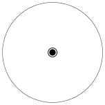
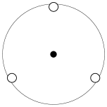
blah

spacer pentagon

trigonal bipyramid

spacer square pyramid

spacer octahedron

spacer trigonal prism

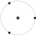
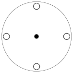
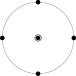
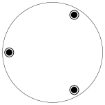
blah

spacer hexagon

pentagonal bipyramid

capped trigonal antiprism

spacer cube

square antiprism

blah

spacer hexagonal bipyramid

spacer augmented trigonal prism

spacer capped square prism

spacer capped square antiprism

bicapped square antiprism

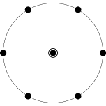
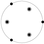
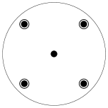
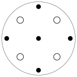
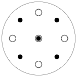
blah

icosahedron

cuboctahedron

dodecahedron

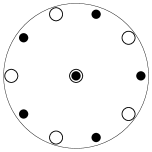
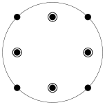
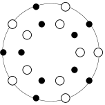
Table 3.1: Candidate crystal structures with $P$ plane waves, specified by their symmetry group $\mathcal{G}$ and Föppl configuration. Bars denote dimensionless equivalents: $\bar{\beta}=\beta\,{\delta\mu}^{2}$, $\bar{\gamma}=\gamma\,{\delta\mu}^{4}$, $\bar{\Omega}=\Omega/({\delta\mu}_{2}^{2}N_{0})$ with $N_{0}=2\bar{\mu}^{2}/\pi^{2}$. $\bar{\Omega}_{\min}$ is the (dimensionless) minimum free energy at ${\delta\mu}={\delta\mu}_{2}$, obtained from (3.32). The phase transition (first order for $\bar{\beta}<0$ and $\bar{\gamma}>0$, second order for $\bar{\beta}>0$ and $\bar{\gamma}>0$) occurs at ${\delta\mu}_{*}$.

	Structure	P	$\mathcal{G}$(Föppl)	$\bar{\beta}$	$\bar{\gamma}$	$\bar{\Omega}_{\min}$	${\delta\mu}_{*}/\Delta_{0}$
1	point	1	$C_{\infty v}$(1)	0.569	1.637	0	0.754
2	antipodal pair	2	$D_{\infty v}$(11)	0.138	1.952	0	0.754
3	triangle	3	$D_{3h}$(3)	-1.976	1.687	-0.452	0.872
4	tetrahedron	4	$T_{d}$(13)	-5.727	4.350	-1.655	1.074
5	square	4	$D_{4h}$(4)	-10.350	-1.538	–	–
6	pentagon	5	$D_{5h}$(5)	-13.004	8.386	-5.211	1.607
7	trigonal bipyramid	5	$D_{3h}$(131)	-11.613	13.913	-1.348	1.085
8	square pyramid	5	$C_{4v}$(14)	-22.014	-70.442	–	–
9	octahedron	6	$O_{h}$(141)	-31.466	19.711	-13.365	3.625
10	trigonal prism	6	$D_{3h}$(33)	-35.018	-35.202	–	–
11	hexagon	6	$D_{6h}$(6)	23.669	6009.225	0	0.754
12	pentagonal	7	$D_{5h}$(151)	-29.158	54.822	-1.375	1.143
	bipyramid
13	capped trigonal	7	$C_{3v}$($13\bar{3}$)	-65.112	-195.592	–	–
	antiprism
14	cube	8	$O_{h}$(44)	-110.757	-459.242	–	–
15	square antiprism	8	$D_{4d}$($4\bar{4}$)	-57.363	-6.866	–	–
16	hexagonal	8	$D_{6h}$(161)	-8.074	5595.528	$-2.8\times 10^{-6}$	0.755
	bipyramid
17	augmented	9	$D_{3h}$($3\bar{3}\bar{3}$)	-69.857	129.259	-3.401	1.656
	trigonal prism
18	capped	9	$C_{4v}$(144)	-95.529	7771.152	-0.0024	0.773
	square prism
19	capped	9	$C_{4v}$($14\bar{4}$)	-68.025	106.362	-4.637	1.867
	square antiprism
20	bicapped	10	$D_{4d}$($14\bar{4}1$)	-14.298	7318.885	$-9.1\times 10^{-6}$	0.755
	square antiprism
21	icosahedron	12	$I_{h}$($15\bar{5}1$)	204.873	145076.754	0	0.754
22	cuboctahedron	12	$O_{h}$($4\bar{4}\bar{4}$)	-5.296	97086.514	$-2.6\times 10^{-9}$	0.754
23	dodecahedron	20	$I_{h}$(5555)	-527.357	114166.566	-0.0019	0.772

Because the LOFF pairing rings have an opening angle $\psi_{0}\simeq 67.1^{\circ}$, no more than nine rings can be arranged on the Fermi surface without any intersection [94, 95]. For this reason we have focussed on crystal structures with nine or fewer waves, but we have included several structures with more waves in order to verify that such structures are not favored. We have tried to analyze a fairly exhaustive list of candidate structures. All five Platonic solids are included in Table 3.1, as is the simplest Archimedean solid, the cuboctahedron. (All other Archimedean solids have even more vertices.) We have analyzed many dihedral polyhedra and polygons: regular polygons, bipyramids, prisms, antiprisms, and various capped or augmented polyhedra. For each crystal structure we list the crystal point group $\mathcal{G}$ and the Föppl configuration of the polyhedron or polygon. The Föppl configuration is a list of the number of vertices on circles formed by intersections of the sphere with consecutive planes perpendicular to the principal symmetry axis of the polyhedron or polygon. We use a modified notation where $a$ or $\bar{a}$ indicates that the points on a given circle are respectively eclipsed or staggered relative to the circle above. Note that polyhedra with several different principal symmetry axes, namely those with $T$, $O$, or $I$ symmetry, have several different Föppl descriptions: for example, a cube is $(44)$ along a fourfold symmetry axis or $(13\bar{3}1)$ along a threefold symmetry axis. (That is, the cube can equally be described as a square prism or a bicapped trigonal antiprism. This should make clear that the singly capped trigonal antiprism of Fig. 3.9 and Table 3.1 is a cube with one vertex removed.)

We do not claim to have analyzed all possible crystal structures, since that is an infinite task. However, there are several classic mathematical problems regarding extremal arrangements of points on a sphere and, although we do not know that our problem is related to one of these, we have made sure to include solutions to these problems. For example, many of the structures that we have evaluated correspond to solutions of Thomson’s problem [110, 94] (lowest energy arrangement of $P$ point charges on the surface of a sphere) or Tammes’s problem [95, 94] (best packing of $P$ equal circles on the surface of a sphere without any overlap). In fact, we include all solutions to the Thomson and Tammes problems for $P\leq 9$. Our list also includes all “balanced” configurations [111] that are possible for nonintersecting rings: a balanced configuration is a set $\mathcal{Q}$ with a rotational symmetry about every ${\mathbf{q}}\in\mathcal{Q}$; this corresponds to an arrangement of particles on a sphere for which the particles are in equilibrium for any two-particle force law.

For each crystal structure, we have calculated the quartic and sextic coefficients $\beta$ and $\gamma$ according to Eqs. (3.26), using methods described in appendix A to calculate all the $J$ and $K$ integrals. To further discriminate among the various candidate structures, we also list the minimum free energy $\Omega_{\min}$ evaluated at the plane-wave instability point ${\delta\mu}={\delta\mu}_{2}$ where $\alpha=0$. To set the scale, note that the BCS state at ${\delta\mu}=0$ has $\Omega_{\rm BCS}=-\mu^{2}\Delta_{0}^{2}/\pi^{2}$, corresponding to $\bar{\Omega}_{\rm BCS}=-0.879$ in the units of Table 3.1. For those configurations with $\beta>0$ and $\gamma>0$, $\Omega_{\min}=0$ at ${\delta\mu}={\delta\mu}_{2}$ and $\Omega_{\min}<0$ for ${\delta\mu}<{\delta\mu}_{2}$, where $\alpha<0$. Thus, we find a second-order phase transition at ${\delta\mu}={\delta\mu}_{2}$. For those configurations with $\beta<0$ and $\gamma>0$, at ${\delta\mu}={\delta\mu}_{2}$ the minimum free energy occurs at a nonzero $\Delta$ with $\Omega_{\min}<0$. (The value of $\Delta$ at which this minimum occurs can be obtained from (3.32).) Because $\Omega_{\min}<0$ at ${\delta\mu}={\delta\mu}_{2}$, if we go to ${\delta\mu}>{\delta\mu}_{2}$, where $\alpha>0$, we lift this minimum until at some ${\delta\mu}_{*}$ it has $\Omega=0$ and becomes degenerate with the $\Delta=0$ minimum. At ${\delta\mu}={\delta\mu}_{*}$, a first-order phase transition occurs. For a very weak first-order phase transition, ${\delta\mu}_{*}\simeq{\delta\mu}_{2}\simeq 0.754\Delta_{0}$. For a strong first-order phase transition, ${\delta\mu}_{*}\gg{\delta\mu}_{2}$ and the crystalline color superconducting phase prevails as the favored ground state over a wider range of ${\delta\mu}$.

3.3.5 Crystal structures with intersecting rings

There are seven configurations in Table 3.1 with very large positive values for $\gamma$. These are precisely the seven configurations that have intersecting pairing rings: the hexagon, hexagonal prism, capped square prism, bicapped square antiprism, icosahedron, cuboctahedron, and dodecahedron. The first two of these include hexagons, and since $\psi_{0}>60^{\circ}$ the rings intersect. The last four of these crystal structures have more than nine rings, meaning that intersections between rings are also inevitable. The capped square prism is an example of a nine-wave structure with intersecting rings. It has a $\gamma$ which is almost two orders of magnitude larger than that of the augmented trigonal prism and the capped square antiprism which, in contrast, are nine wave structures with no intersecting rings. Because of their very large $\gamma$’s all the structures with intersecting rings have either second-order phase transitions or very weak first-order phase transitions occurring at a ${\delta\mu}_{*}\simeq{\delta\mu}_{2}$. At ${\delta\mu}={\delta\mu}_{2}$, all these crystal structures have $\Omega_{\min}$ very close to zero. Thus, as our analysis of two plane waves led us to expect, we conclude that these crowded configurations with intersecting rings are disfavored.

3.3.6 “Regular” crystal structures

At the opposite extreme, we see that there are several structures that have negative values of $\gamma$: the square, square pyramid, square antiprism, trigonal prism, capped trigonal antiprism, and cube. Our analysis demonstrates that the transition to all these crystal structures (as to those with $\beta<0$ and $\gamma>0$) is first order. But, we cannot evaluate $\Omega_{\min}$ or ${\delta\mu}_{*}$ because, to the order we are working, $\Omega$ is unbounded from below. For each of these crystal structures, we could formulate a well-posed (but difficult) variational problem in which we make a variational ansatz corresponding to the structure, vary, and find $\Omega_{\min}$ without making a Ginzburg-Landau approximation. It is likely, therefore, that within the Ginzburg-Landau approximation $\Omega$ will be stabilized at a higher order than the sextic order to which we have worked.

Of the sixteen crystal structures with no intersecting rings, there are seven that are particularly favored by the combinatorics of Eqs. (3.26). It turns out that these seven crystal structures are precisely the six that we have found with $\gamma<0$, plus the octahedron, which is the most favored crystal structure among those with $\gamma>0$. As discussed earlier, more terms contribute to the rhombic and hexagonal sums in Eqs. (3.26) when the ${\mathbf{q}}$’s are arranged in such away that their vertices form rectangles, trapezoids, and cuboids inscribed in the sphere $|{\mathbf{q}}|=q_{0}$. Thus the square itself fares well, as do the square pyramid, square antiprism, and trigonal prism which contain one, two, and three rectangular faces, respectively. The octahedron has three square cross sections. However, the cube is the outstanding winner because it has six rectangular faces, six rectangular cross sections, and also allows the five-corner arrangements described previously. The capped trigonal antiprism in Table 3.1 is a cube with one vertex removed. This seven-wave crystal has almost as many waves as the cube, and almost as many combinatorial advantages as the cube, and it turns out to have the second most negative $\gamma$.

With eight rings, the cube is close to the maximum packing for nonintersecting rings with opening angle $\psi_{0}\simeq 67.1^{\circ}$. Although nine rings of this size can be packed on the sphere, adding a ninth ring to the cube and deforming the eight rings into a cuboid, as we have done with the capped square prism, necessarily results in intersecting rings and the ensuing cost overwhelms the benefits of the cuboidal structure. To form a nine-ring structure with no intersections requires rearranging the eight rings, spoiling the favorable regularities of the cuboid. Therefore a nine-ring arrangement is actually less favorable than the cuboid, even though it allows one more plane wave. We see from Table 3.1 that $\gamma$ for the cube is much more negative than that for any of the other combinatorially favored structures. The cube is our winner, and we understand why.

To explore the extent to which the cube is favored, we can compare it to the octahedron, which is the crystal structure with $\gamma>0$ for which we found the strongest first-order phase transition, with the largest ${\delta\mu}_{*}$ and the deepest $\Omega_{\min}$. The order $\Delta^{6}$ free energy we have calculated for the cube is far below that for the octahedron at all values of $\Delta$. To take an extreme example, at ${\delta\mu}={\delta\mu}_{2}$ the octahedron has $\bar{\Omega}_{\min}=-13.365$ at $\Delta=1.263{\delta\mu}_{2}=0.953\Delta_{0}$ whereas for the cube we find that $\bar{\Omega}=-2151.5$ at this $\Delta$. As another example, suppose that we arbitrarily add $+{\textstyle\frac{1}{4}}800\Delta^{8}/{\delta\mu}^{8}$ to the $\bar{\Omega}$ of the cube. In this case, at ${\delta\mu}={\delta\mu}_{2}$ we find that the cube has $\bar{\Omega}_{\min}=-32.5$ at $\Delta=0.656\Delta_{0}$ and is thus still favored over the octahedron, even though we have not added any $\Delta^{8}$ term to the free energy of the octahedron. These numerical exercises demonstrate the extraordinary robustness of the cube, but should not be taken as more than qualitative. We do not know at what $\Delta$ and at what value $\Omega_{\min}$ the true free energy for the cube finds its minimum. However, because the qualitative features of the cube are so favorable we expect that it will have a deeper $\Omega_{\min}$ and a larger ${\delta\mu}_{*}$ than the octahedron. Within the Ginzburg-Landau approximation, the octahedron already has $\Delta=0.953\Delta_{0}$ and a deep $\bar{\Omega}_{\min}=-13.365$, about fifteen times deeper than $\bar{\Omega}_{\rm BCS}=-0.879$ for the BCS state at ${\delta\mu}=0$ .

Even if we were to push the Ginzburg-Landau analysis of the cube to higher order and find a stable $\Omega_{\min}$, we would not be able to trust such a result quantitatively. Because it predicts a strong first-order phase transition, the Ginzburg-Landau approximation predicts its own quantitative demise. What we have learned from it, however, is that there are qualitative reasons that make the cube the most favored crystal structure of them all. And, to the extent that we can trust the quantitative calculations qualitatively, they indicate that the first-order phase transition results in a state with $\Delta$ and $\Omega_{\min}$ comparable to those of the BCS phase, and occurs at a ${\delta\mu}_{*}\gg{\delta\mu}_{2}$.

3.3.7 Varying continuous degrees of freedom

None of the regularities of the cube which make it so favorable are lost if it is deformed continuously into a cuboid, slightly shorter or taller than it is wide, as long as it is not deformed so much as to cause rings to cross. Next, we investigate this and some of the other possible continuous degrees of freedom present in a number of the crystal structures we have described above.

So far we have neglected the fact, mentioned at the start of this section, that some of the candidate structures have multiple orbits under the action of the point group $\mathcal{G}$. These structures include the square pyramid, the four bipyramids, and the five capped or augmented structures listed in Table 3.1; all have two orbits except for the three singly capped crystal structures, which have three orbits. For these multiple-orbit structures each orbit should have a different gap parameter but in Table 3.1 we have assumed that all the gaps are equal. We have, however, analyzed each of these structures upon assuming different gaps, searching for a minimum of the free energy in the two- or three-dimensional parameter space of gaps. In most cases, the deepest minimum is actually obtained by simply eliminating one of the orbits from the configuration (i.e. let $\Delta=0$ for that orbit); the resultant structure with one less orbit appears as another structure in Table 3.1. For example, the bicapped square antiprism has two orbits: the first is the set of eight ${\mathbf{q}}$’s forming a square antiprism, the second is the antipodal pair of ${\mathbf{q}}$’s forming the two “caps” of the structure. Denote the gaps corresponding to these two orbits as $\Delta_{1}$ and $\Delta_{2}$. This structure is overcrowded with intersecting rings, so it is not surprising to find that a lower-energy configuration is obtained by simply letting $\Delta_{2}=0$, which gives the “uncapped” square antiprism. Configurations with fewer orbits are generally more favorable, with only three exceptions known to us: the trigonal bipyramid is favored over the triangle or the antipodal pair; the square pyramid is favored over the square or the point; and the capped trigonal antiprism is favored over any of the structures that can be obtained from it by removing one or two orbits. For these configurations, Table 3.1 lists the results for $\Delta_{1}=\Delta_{2}\,(=\Delta_{3})$; the numbers can be slightly improved with $\Delta_{1}\neq\Delta_{2}\,(\neq\Delta_{3})$ but the difference is unimportant.

For some configurations in Table 3.1 the positions of the points are completely fixed by symmetry while for others the positions of the points can be varied continuously, while still maintaining the point-group symmetry of the structure. For example, with the square pyramid we can vary the latitude of the plane that contains the inscribed pyramid base. Similarly, with the various polygonal prism and antiprism structures (and associated cappings and augmentations), we can vary the latitudes of the inscribed polygons (equivalently, we can vary the heights of these structures along the principal symmetry axis). For each structure that has such degrees of freedom, we have scanned the allowed continuous parameter space to find the favored configuration. Table 3.1 then shows the results for this favored configuration, and the latitude angles describing the favored configuration are given as footnotes. However, if the structure always has overlapping rings regardless of its deformation, then either no favorite configuration exists or the favorite configuration is a degenerate one that removes the overlaps by changing the structure. There are two instances where this occurs: the capped square prism can be deformed into a square pyramid by shrinking the height of the square prism to zero, and the bicapped square antiprism can be deformed into an antipodal pair by moving the top and bottom square faces of the antiprism to the north and south poles, respectively. For these structures, Table 3.1 just lists results for an arbitrarily chosen nondegenerate configuration.

\psfrag{x1}[tc][tc]{\small$10^{\circ}$}\psfrag{x2}[tc][tc]{\small$20^{\circ}$}\psfrag{x3}[tc][tc]{\small$30^{\circ}$}\psfrag{x4}[tc][tc]{\small$40^{\circ}$}\psfrag{x5}[tc][tc]{\small$50^{\circ}$}\psfrag{x6}[tc][tc]{\small$60^{\circ}$}\psfrag{x7}[tc][tc]{\small$70^{\circ}$}\psfrag{x8}[tc][tc]{\small$80^{\circ}$}\psfrag{x9}[tc][tc]{\small$90^{\circ}$}\psfrag{x10}[tc][tc]{\small$50^{\circ}$}\psfrag{x11}[tc][tc]{\small$55^{\circ}$}\psfrag{x12}[tc][tc]{\small$60^{\circ}$}\psfrag{x13}[tc][tc]{\small$65^{\circ}$}\psfrag{y1}[rc][rc]{\small 3000}\psfrag{y2}[rc][rc]{\small 6000}\psfrag{y3}[rc][rc]{\small 9000}\psfrag{y4}[rc][rc]{\small 12000}\psfrag{y5}[rc][rc]{\small 15000}\psfrag{y6}[rc][rc]{\small 30}\psfrag{y7}[rc][rc]{\small 60}\psfrag{y8}[rc][rc]{\small 90}\psfrag{y9}[rc][rc]{\small 120}\psfrag{y10}[rc][rc]{\small 150}\psfrag{xlabel}{$\theta$}\psfrag{ylabel}{$\gamma(\theta){\delta\mu}^{4}$}\includegraphics[width=433.62pt]{squareantiprismplot.eps}

Figure 3.10: The sextic free energy coefficient $\gamma$ for the square antiprism as a function of the polar (latitude) angle $\theta$ of the top square facet. (The polar angle of the bottom square facet is $\pi-\theta$.) The inset plot shows the detail in the range of $\theta$ where no rings intersect. Solid and dashed vertical lines indicate the positions of primary and secondary singularities as discussed in the text (other secondary singularities occur, but are not discernible on the plot).

A typical parameter scan is shown in Fig, 3.10, where we have plotted $\gamma$ for the square antiprism as a function of the polar angle $\theta$ of the top square facet (the polar angle of the bottom square facet is $\pi-\theta$). As we expect, $\gamma$ is very large in regions where any rings intersect, and we search for a minimum of $\gamma$ in the region where no rings intersect. The plot has a rather complicated structure of singularities and discontinuities; these features are analogous to those of Fig. 3.8, and as there they arise as a result of the double limit we are taking. Primary singularities occur at critical angles where pairing rings are mutually tangent on the Fermi surface. Secondary singularities occur where rings corresponding to harmonic ${\mathbf{q}}$’s, obtained by taking sums and differences of the fundamental ${\mathbf{q}}$’s that define the crystal structure, are mutually tangent. Such ${\mathbf{q}}$’s arise in the calculation of $J$ and $K$ because these calculations involve momenta corresponding to various diagonals of the rhombus and hexagon in Fig. 3.6.

In addition to varying the latitudes of the Föppl planes in various structures, we varied “twist angles”. For example, we explored the continuous degree of freedom that turns a cube into a square antiprism, by twisting the top square relative to the bottom square by an angle $\phi$ ranging from $0^{\circ}$ to $45^{\circ}$. In Fig. 3.11, we show a parameter scan in which we simultaneously vary the twist angle $\phi$ and the latitudes of the square planes in such a way that the scan interpolates linearly from the cube to the most favorable square antiprism of Table 3.1. In this parameter scan, we find a collection of secondary singularities and one striking fact: $\gamma$ is much more negative when the twist angle is zero (i.e. for the cube itself) than for any nonzero value. For the cube, $\gamma=-459.2/{\delta\mu}^{4}$, whereas the best one can do with a nonzero twist is $\gamma=-64.2/{\delta\mu}^{4}$, which is the result for an infinitesimal twist angle. Thus, any nonzero twist spoils the regularities of the cube that contribute to its combinatorial advantage, and this has a dramatic and unfavorable effect on the free energy.

\psfrag{5}[tc][tc]{\small$5^{\circ}$}\psfrag{10}[tc][tc]{\small$10^{\circ}$}\psfrag{15}[tc][tc]{\small$15^{\circ}$}\psfrag{20}[tc][tc]{\small$20^{\circ}$}\psfrag{25}[tc][tc]{\small$25^{\circ}$}\psfrag{30}[tc][tc]{\small$30^{\circ}$}\psfrag{35}[tc][tc]{\small$35^{\circ}$}\psfrag{40}[tc][tc]{\small$40^{\circ}$}\psfrag{45}[tc][tc]{\small$45^{\circ}$}\psfrag{-500}[rc][rc]{\small-500}\psfrag{-400}[rc][rc]{\small-400}\psfrag{-300}[rc][rc]{\small-300}\psfrag{-200}[rc][rc]{\small-200}\psfrag{-100}[rc][rc]{\small-100}\psfrag{-100}[rc][rc]{\small-100}\psfrag{100}[rc][rc]{\small 100}\psfrag{200}[rc][rc]{\small 200}\psfrag{xlabel}{$\phi$}\psfrag{ylabel}{$\gamma(\phi){\delta\mu}^{4}$}\psfrag{arrowlabel1}[lb][lt]{cube}\psfrag{arrowlabel2}[tc][rb]{\mbox{square antiprism}}\includegraphics[width=361.34999pt]{twistfig.eps}

Figure 3.11: The sextic free energy coefficient $\gamma$ for a scan that linearly interpolates from the cube (twist angle $\phi=0$) to the square antiprism of Table 3.1 (twist angle $\phi=45^{\circ}$). Dashed vertical lines indicate secondary singularities.

Finally, we have scanned the parameter space of a generic cuboid to see how this compares to the special case of a cube. That is, we vary the height of the cuboid relative to its width, without introducing any twist. This continuous variation does not reduce the combinatorial advantage of the crystal structure. As expected, therefore, we find that as long as the cuboid has no intersecting rings, it has a free energy that is very similar to that of the cube itself. Any cuboid with intersecting rings is very unfavorable. In the restricted parameter space of nonintersecting cuboidal arrangements, the cuboid with the most negative free energy is a square prism with a polar angle of $51.4^{\circ}$ for the top square face. (For this polar angle the pairing rings corresponding to the four corners of the square are almost mutually tangent.) This prism is slightly taller than a perfect cube, which has a polar angle of $54.7^{\circ}$. The free energy coefficients of the best cuboid are $\beta=-111.563/({\delta\mu})^{2}$, $\gamma=-463.878/({\delta\mu})^{4}$. These coefficients differ by less than $1\%$ from those for the cube, given in Table 3.1. There is no significant difference between the cube and this very slightly more favorable cuboid: all the qualitative arguments that favor the cube favor any cuboid with no intersecting rings equally well. We therefore expect that if we could determine the exact (rather than Ginzburg-Landau) free energy, we would find that the favored crystal structure is a cuboid with a polar angle somewhere between $51.4^{\circ}$ and $56.5^{\circ}$, as this is the range for which no rings intersect. We expect no important distinction between the free energy of whichever cuboid in this narrow range happens to be favored and that of the cube itself.

3.4 Conclusions

We have argued that the cube crystal structure is the favored ground state at zero temperature near the plane-wave instability point ${\delta\mu}={\delta\mu}_{2}$. By the cube we mean a crystal structure constructed as the sum of eight plane waves with wave vectors pointing towards the corners of a cube. The qualitative points (which we have demonstrated in explicit detail via the analysis of many different crystal structures) that lead us to conclude that the cube is the winner are:

• The quadratic term in the Ginzburg-Landau free energy wants a $|{\mathbf{q}}|$ such that the pairing associated with any single choice of $\hat{\mathbf{q}}$ occurs on a ring with opening angle $\psi_{0}\simeq 67.1^{\circ}$ on each Fermi surface.

• The quadratic term in the Ginzburg-Landau free energy favors condensation with many different wave vectors, and thus many different pairing rings on the Fermi surfaces. However, the quartic and sextic terms in the free energy strenuously prohibit the intersection of pairing rings. No more than nine rings with opening angle $67.1^{\circ}$ can be placed on the sphere without overlap.

• The quartic and sextic terms favor regular crystal structures, for example those that include many different sets of wave vectors whose tips form rectangles. None of the nine-wave structures with no intersections between pairing rings are regular in the required sense. The cube is a very regular eight-wave crystal structure.

Quantitatively, we find that a cube (actually, a cuboid that is only slightly taller than it is wide) has by far the most negative Ginzburg-Landau free energy, to sextic order, of all the many crystal structures we have investigated. For the cube structure, the eight ${\mathbf{q}}$ vectors are the eight shortest vectors in the reciprocal lattice of a face-centered-cubic crystal. Therefore, we find that $\Delta({\mathbf{x}})$ exhibits face-centered-cubic (FCC) symmetry. The explicit form of the gap function $\Delta({\mathbf{x}})$ is shown in equation (1.25), and a unit cell of the FCC crystal is shown in figure 1.6.

Our Ginzburg-Landau analysis predicts a first-order phase transition to the cubic crystalline color superconductor at some ${\delta\mu}={\delta\mu}_{*}$. The fact that we predict a first-order phase transition means that the Ginzburg-Landau analysis cannot be trusted quantitatively. Furthermore, at order $\Delta^{6}$, which is as far as we have gone, the Ginzburg-Landau free energy for the cube is unbounded from below. We therefore have no quantitative prediction of ${\delta\mu}_{*}$ or the magnitude of $\Delta$. The best we can do is to note that the cube is significantly favored over the octahedron, for which the order $\Delta^{6}$ Ginzburg-Landau analysis predicts ${\delta\mu}_{*}\simeq 3.6\Delta_{0}$ and predicts that at ${\delta\mu}={\delta\mu}_{2}=0.754\Delta_{0}$, the gap is $\Delta\simeq 0.95\Delta_{0}$ and the condensation energy is larger than that in the BCS state by a factor of about fifteen. As we have warned repeatedly, these numbers should not be trusted quantitatively: because the Ginzburg-Landau approximation predicts a strong first-order phase transition, it predicts its own breakdown. We have learned several qualitative lessons from it, however:

• We have understood the qualitative reasons that make the cube the most favored crystal structure of them all. It has the largest number of pairing rings that can be “regularly” arranged on the Fermi surface without ring overlaps.

• The cube structure has an unstable Ginzburg-Landau free energy. As a result the Ginzburg-Landau analysis cannot give quantitative results, but the large instability suggests a robust crystalline phase. The gap parameter $\Delta$ for the crystalline phase could be comparable to the gap $\Delta_{0}$ for the BCS phase. Similarly, the condensation energy by which the crystalline phase is favored over unpaired quark matter at ${\delta\mu}\neq 0$ could be comparable to that for the BCS phase at ${\delta\mu}=0$.

• Although we began our analysis in the vicinity of the second-order plane-wave instability point ${\delta\mu}_{2}$, the transition to the crystalline phase is strongly first-order and occurs at a ${\delta\mu}_{*}\gg{\delta\mu}_{2}$. The emergence of a first-order transition from a study of a second-order point has a precedent in the Ginzburg-Landau analysis for the liquid-solid transition [93].

• We learn that the crystalline color superconductivity window ${\delta\mu}_{1}<{\delta\mu}<{\delta\mu}_{*}$ is large. Because ${\delta\mu}_{2}$ is not much larger than ${\delta\mu}_{1}$, the original LOFF window ${\delta\mu}_{1}<{\delta\mu}<{\delta\mu}_{2}$ wherein the single plane-wave condensate is possible is quite narrow. We have learned, however, that ${\delta\mu}_{*}\gg{\delta\mu}_{2}$. Furthermore, because the condensation energy of the crystalline phase is so robust, much greater than that for the single plane wave and likely comparable to that for the BCS phase, the value of ${\delta\mu}_{1}$, the location of the transition between the crystalline phase and the BCS phase, will be significantly depressed. So the LOFF window is considerably widened in both directions.

• Given the robustness of the FCC crystalline phase in our two flavor model, in real QCD with three flavors of quarks we can expect that the crystalline phase will occupy a large regions of the $(T,\mu)$ phase diagram of figure 1.1.

blah

Chapter 4 Single Color and Single Flavor Color Superconductivity

4.1 Overview

There are nine types of quark (3 colors, 3 flavors) in dense quark matter. In general we expect that all nine quarks will find attractive channels in which to form Cooper pairs, because any pairing lowers the free energy by BCS condensation. The color-flavor-locked (CFL) phase directly accomplishes this feat, but for non-CFL phases of color superconductivity that occur at intermediate densities as in figure 1.1, it is not obvious how the system contrives to pair all nine quarks. Here we speculate on some of the contrivances that might occur.

In the 2SC phase (which seems unlikely to occur in neutral quark matter), only two colors and two flavors pair, leaving five “orphaned” quarks: the blue up and down quarks, and all three colors of strange quark. In this context it has been proposed that the blue up and down quarks could pair together in a single-color condensate [9, 98], and all the strange quarks could pair together in a single-flavor condensate which involves all three colors [63, 8].

Single-flavor pairing can also occur in the limit of very large separation between the Fermi surfaces for the different flavors. In this context the system will abandon inter-species pairing and form $\langle uu\rangle$, $\langle dd\rangle$, and $\langle ss\rangle$ condensates. Each could involve three colors (e.g. in a color-spin-locked (CSL) phase [63]) and therefore all nine quarks are paired.

In the LOFF crystalline phase, so far we have only discussed the two-flavor situation of pairing between up and down quarks. This is a “2SC-LOFF” phase: just like the spatially-uniform 2SC phase, it pairs only two colors and two flavors and leaves five orphaned quarks. In a real three-flavor context, the crystalline phase could involve $ud$, $us$, and $ds$ pairs, thus involving all nine quarks in a “CFL-LOFF” phase. Alternatively, the three-flavor LOFF state might involve only $ud$ and $us$ pairs, i.e. it might only pair quarks with adjacent Fermi surfaces (recall that in neutral quark matter the Fermi momenta are split with $p_{F}^{s}<p_{F}^{u}<p_{F}^{d}$). In this case, the $ud$ pairing could involve $r$ and $g$ quarks, and the $us$ pairing could involve $r$ and $b$ quarks, and two quarks are orphaned: the blue down quark and the green strange quark. These lonely quarks might resort to self-pairing if the QCD interaction permits an attraction in this channel (we will see that it does in some NJL models, if the quark is heavy enough).

In this chapter we survey a large catalog of different color-flavor-spin channels for diquark condensation [62]. This catalog includes the single-color and/or single-flavor pairing channels that are mentioned in the various scenarios described above [8, 9, 63, 98]. We consider only translationally invariant phases, but many of the condensates in our survey have non-zero spin, and therefore spontaneously break rotational invariance. In section 4.2 we identify the attractive channels using NJL models with four-fermion interactions based on instantons, magnetic gluons, and combined electric and magnetic gluons. In section 4.3 we solve the NJL mean-field gap equations for the channels that are attractive. In section 4.4 we investigate the quasiquark dispersion relations for the spin-one condensates. The quasiquark energy gaps are anisotropic and gapless modes can occur at the poles or at the equator of the Fermi surface. Finally in section 4.5, we summarize the results, suggest directions for further study, and speculate about implications for the physics of compact stars.

4.2 Mean-field survey of quark pairing channels

4.2.1 Calculation

To see which channels are attractive we perform a mean-field calculation of the pairing energy for a wide range of condensation patterns. We write the NJL Hamiltonian in the form

$$\begin{array}[]{rcl}H&=&H_{\rm free}+H_{\rm interaction}\\[4.30554pt] H_{\rm free}&=&{\bar{\psi}}({\partial\kern-5.50003pt/}-\mu\gamma_{0}+m)\psi\\[4.30554pt] H_{\rm interaction}&=&{\psi^{\dagger}}_{\alpha}^{ia}\psi^{\beta b}_{j}{\psi^{\dagger}}_{\gamma}^{kc}\psi^{\delta d}_{l}\,\,{\cal H}^{\alpha}_{ia}{\,}_{\beta b}^{j}{\,}^{\gamma}_{kc}{\,}_{\delta d}^{l}\ ,\end{array}$$ (4.1)

where color indices are $\alpha,\beta,\gamma,\delta$, flavor indices are $i,j,k,l$, spinor indices are $a,b,c,d$. The four-fermion interaction is supposed to be a plausible model of QCD, so in the interaction kernel ${\cal H}$ we include three terms, with the color-flavor-spinor structure of a two-flavor instanton, electric gluon exchange, and magnetic gluon exchange,

$$\begin{array}[]{rcl}{\cal H}&=&{\cal H}_{\rm elec}+{\cal H}_{\rm mag}+{\cal H}_{\rm inst}\\[4.30554pt] {\cal H}_{\rm elec}&=&\phantom{-}\frac{3}{8}G_{E}\,\,\delta_{i}^{j}\delta_{k}^{l}\,\,\delta_{ab}\delta_{cd}\,\,\frac{2}{3}(3\delta^{\alpha}_{\delta}\delta^{\gamma}_{\beta}-\delta^{\alpha}_{\beta}\delta^{\gamma}_{\delta})\\[4.30554pt] {\cal H}_{\rm mag}&=&\phantom{-}\frac{3}{8}G_{M}\,\,\delta_{i}^{j}\delta_{k}^{l}\,\,\sum_{n=1}^{3}[\gamma_{0}\gamma_{n}]_{ab}[\gamma_{0}\gamma_{n}]_{cd}\,\,\frac{2}{3}(3\delta^{\alpha}_{\delta}\delta^{\gamma}_{\beta}-\delta^{\alpha}_{\beta}\delta^{\gamma}_{\delta})\\[4.30554pt] {\cal H}_{\rm inst}&=&-\frac{3}{4}G_{I}\,\,\varepsilon_{ik}\varepsilon^{jl}\,\,{\textstyle\frac{1}{4}}\Bigl{(}[\gamma_{0}(1+\gamma_{5})]_{ab}[\gamma_{0}(1+\gamma_{5})]_{cd}+[\gamma_{0}(1-\gamma_{5})]_{ab}[\gamma_{0}(1-\gamma_{5})]_{cd}\Bigr{)}\\ &&\phantom{-\frac{3}{4}G_{I}}\frac{2}{3}(3\delta^{\alpha}_{\beta}\delta^{\gamma}_{\delta}-\delta^{\alpha}_{\delta}\delta^{\gamma}_{\beta})\end{array}$$ (4.2)

We consider condensates that factorize into separate color, flavor, and Dirac tensors (i.e. that do not show “locking”) and calculate their binding energy by contracting them with (4.2).

There is no Fierzing ambiguity in this procedure. For a given pairing pattern $X$, the condensate is

$$\langle\psi^{\beta b}_{j}\psi^{\delta d}_{l}\rangle^{\vphantom{y}}_{1PI}=\Delta(X)\mathfrak{C}_{(X)}^{\beta\delta}\mathfrak{F}^{\vphantom{\beta}}_{(X)jl}\Gamma_{(X)}^{bd\vphantom{\beta}}~{}.$$ (4.3)

We can then calculate the interaction (“binding”) energy of the various condensates,

$$H=-\sum_{X}\Delta(X)^{2}\Bigl{(}S^{(X)}_{\rm elec}G_{E}+S^{(X)}_{\rm mag}G_{M}+S^{(X)}_{\rm inst}G_{I}\Bigr{)}$$ (4.4)

The binding strengths $S^{(X)}_{\rm interaction}$ give the strength of the self-interaction of the condensate $X$ due to the specified part of the interaction Hamiltonian.

4.2.2 Properties of the pairing channels

In Table 4.1 we list the the simple (translationally invariant, factorizable) channels available for quark pairing. The meanings of the columns are as follows.

1. Color: two quarks either make an antisymmetric color triplet (which requires quarks of two different colors) or a symmetric sextet (which can occur with quarks of two different colors, and also if both quarks have the same color). For the $\bar{\bf 3}_{A}$ we use $\mathfrak{C}^{\beta\delta}=\varepsilon^{\beta\delta}$ in Eq. (4.3). For the ${\bf 6}_{S}$ we use a single-color representative $\mathfrak{C}^{\beta\delta}=\delta^{\beta,1}\delta^{\delta,1}$ in Eq. (4.3).

2. Flavor: two quarks either make an antisymmetric flavor singlet (which requires quarks of two different flavors) or a symmetric triplet (which can occur with quarks of two different flavors, and also if both quarks have the same flavor). For the ${\bf 1}_{A}$ we use $\mathfrak{F}_{jl}=\sigma^{2}_{jl}$ and for the ${\bf 3}_{S}$ we use $\mathfrak{F}_{jl}=\sigma^{1}_{jl}$ in (4.3).

3. Spin, parity: since the chemical potential explicitly breaks the Lorentz group down to three-dimensional rotations and translations, it makes sense to classify condensates by their total angular momentum quantum number $j$ and parity.

4. Dirac: This column gives the Dirac matrix structure $\Gamma^{bd}$ used in (4.3), so the condensate is $\psi^{T}\Gamma\psi$. We also designate each condensate as “LL” (even number of gamma matrices, so pairs same-chirality quarks) or “LR” (odd number of gamma matrices, so pairs opposite-chirality quarks).

5. BCS-enhancement: Condensates that correspond to pairs of particles or holes near the Fermi surface have a BCS singularity in their gap equation that guarantees a solution, no matter how weak the coupling. To see which condensates have such a BCS enhancement, we expanded the field operators in terms of creation and annihilation operators (see Appendix B.3). The order of the coefficient of the $a({\mathbf{p}})a(-{\mathbf{p}})$ and $b^{\dagger}({\mathbf{p}})b^{\dagger}(-{\mathbf{p}})$ terms is given in the table. ${\cal O}(1)$ means BCS-enhanced, $0$ means not BCS-enhanced. In the $C\gamma_{0}\gamma_{5}$ condensate the coefficient goes to zero as the quark mass goes to zero (hence it is labelled “${\cal O}(m)$” in the table) meaning that the channel loses its BCS enhancement in the chiral limit. This is discussed further in Appendix B.3.

6. Binding strength: For each channel we show the binding strength for the instanton interaction, the full (electric plus magnetic) gluon, which could reasonably be used at medium density, and for the magnetic gluon alone, which is known to dominate at ultra-high density [6, 12]. Channels with a positive binding strength and BCS enhancement will always support pairing (the gap equation always has a solution, however weak the couplings $G_{I},G_{E},G_{M}$). Other things being equal, the pairing with the largest binding strength will have the lowest free energy, and is the one that will actually occur.

It may seem strange that there are entries in the table with angular momentum $j=1$ and an antisymmetric Dirac structure ($C\gamma_{3}\gamma_{5}$), and with $j=0$ but a symmetric Dirac structure ($C\gamma_{0}$). If all the angular momentum came from spin this would be impossible. But even though there are no explicit spatial derivatives in the diquark operators, there can still be orbital angular momentum. In Appendix B.3 the angular momentum content of the particle-particle component of the condensates is analyzed into its spin and orbital content. We see, for example, that $C\gamma_{3}\gamma_{5}$ has an antisymmetric space wavefunction ($l=1$) and a symmetric spin wavefunction ($s=1$), combined to give an antisymmetric $j=1$.

4.2.3 Results

Structure of condensate							Binding strength
							instanton	gluon
color	flavor	$j$	parity	Dirac		BCS enhance- ment	$S_{\rm inst}$	full $S_{\rm elec}$ +$S_{\rm mag}$	mag. only $S_{\rm mag}$
$\bar{\bf 3}_{A}$	${\bf 1}_{A}$	$0_{A}$	$+$	$C\gamma_{5}$	LL	${\cal O}(1)$	$+64$	$+64$	$+48$
$\bar{\bf 3}_{A}$	${\bf 1}_{A}$	$0_{A}$	$-$	$C$	LL	${\cal O}(1)$	$-64$	$+64$	$+48$
$\bar{\bf 3}_{A}$	${\bf 1}_{A}$	$0_{A}$	$+$	$C\gamma_{0}\gamma_{5}$	LR	${\cal O}(m)$	0	$-32$	$-48$
$\bar{\bf 3}_{A}$	${\bf 1}_{A}$	$1_{A}$	$-$	$C\gamma_{3}\gamma_{5}$	LR	${\cal O}(1)$	0	$+32$	$+16$
${\bf 6}_{S}$	${\bf 1}_{A}$	$1_{S}$	$-$	$C\sigma_{03}\gamma_{5}$	LL	${\cal O}(1)$	$-16$	0	$+4$
${\bf 6}_{S}$	${\bf 1}_{A}$	$1_{S}$	$+$	$C\sigma_{03}$	LL	${\cal O}(1)$	$+16$	0	$+4$
${\bf 6}_{S}$	${\bf 1}_{A}$	$0_{S}$	$-$	$C\gamma_{0}$	LR	0	0	$+8$	$+12$
${\bf 6}_{S}$	${\bf 1}_{A}$	$1_{S}$	$+$	$C\gamma_{3}$	LR	${\cal O}(1)$	0	$-8$	$-4$
$\bar{\bf 3}_{A}$	${\bf 3}_{S}$	$1_{S}$	$-$	$C\sigma_{03}\gamma_{5}$	LL	${\cal O}(1)$	0	0	$-16$
$\bar{\bf 3}_{A}$	${\bf 3}_{S}$	$1_{S}$	$+$	$C\sigma_{03}$	LL	${\cal O}(1)$	0	0	$-16$
$\bar{\bf 3}_{A}$	${\bf 3}_{S}$	$0_{S}$	$-$	$C\gamma_{0}$	LR	0	0	$-32$	$-48$
$\bar{\bf 3}_{A}$	${\bf 3}_{S}$	$1_{S}$	$+$	$C\gamma_{3}$	LR	${\cal O}(1)$	0	$+32$	$+16$
${\bf 6}_{S}$	${\bf 3}_{S}$	$0_{A}$	$+$	$C\gamma_{5}$	LL	${\cal O}(1)$	0	$-16$	$-12$
${\bf 6}_{S}$	${\bf 3}_{S}$	$0_{A}$	$-$	$C$	LL	${\cal O}(1)$	0	$-16$	$-12$
${\bf 6}_{S}$	${\bf 3}_{S}$	$0_{A}$	$+$	$C\gamma_{0}\gamma_{5}$	LR	${\cal O}(m)$	0	$+8$	$+12$
${\bf 6}_{S}$	${\bf 3}_{S}$	$1_{A}$	$-$	$C\gamma_{3}\gamma_{5}$	LR	${\cal O}(1)$	0	$-8$	$-4$

Table 4.1: Binding strengths of diquark channels in NJL models in the mean-field approximation. The first 6 columns specify the channels, and the last 3 columns give their attractiveness in NJL models with various types of four-fermion vertex: 2-flavor instanton, single gluon exchange, single magnetic gluon exchange (expected to dominate at higher density). See equations (4.3) and (4.4) and subsequent explanation.

The results of the binding strength calculation are shown in Table 4.1. The first block is antisymmetric in flavor and color, and so describes pairing of two flavors and two colors. The second block is for two flavors and one color, the third for one flavor and two colors, and the final block is for one color and one flavor.

Certain features can be easily understood: the flavor-symmetric condensates all have zero instanton binding energy, because the instanton vertex is flavor-antisymmetric in the incoming quarks. The gluonic vertices give the same results for $C\gamma_{5}$ as for $C$, and for $C\sigma_{03}\gamma_{5}$ as for $C\sigma_{03}$, because the gluonic interaction is invariant under $U(1)_{A}$ transformations, under which the LL condensates transform into each other ($C\gamma_{5}\rightleftharpoons C$ and $C\sigma_{03}\gamma_{5}\rightleftharpoons C\sigma_{03}$) while the LR condensates are invariant. We see that there are many attractive channels:

• Two colors and two flavors ($\bar{\bf 3}_{A}$,${\bf 1}_{A}$,$\ldots$).
  The strongly attractive channel ($\bar{\bf 3}_{A}$,${\bf 1}_{A}$,0,$+$)($C\gamma_{5}$) is the 2SC and CFL quark Cooper pairing pattern, and has been extensively studied. The gap is large enough that even species with different masses, whose Fermi momenta are quite far apart, can pair (hence the CFL phase which pairs red and green $u$ and $d$, red and blue $u$ and $s$, and green and blue $d$ and $s$ in this channel). Its parity partner ($\bar{\bf 3}_{A}$,${\bf 1}_{A}$,0,$-$)($C$) is disfavored by instantons, and is therefore unlikely to occur at phenomenologically interesting densities. The additional channel ($\bar{\bf 3}_{A}$,${\bf 1}_{A}$,1,$-$)($C\gamma_{3}\gamma_{5}$) is more weakly attractive and also breaks rotational invariance, and is therefore expected to be even less favored. This is confirmed by gap equation calculations (Fig. 4.2) which show that its gap is smaller by a factor of 10 to 100.

• One color, two flavors (${\bf 6}_{S}$,${\bf 1}_{A}$,$\ldots$).
  It is generally emphasized that the quark-quark interaction is attractive in the color-antisymmetric $\bar{\bf 3}_{A}$ channel. But, as we see in table 4.1, the color-symmetric (${\bf 6}_{S}$,${\bf 1}_{A}$,1,+)($C\sigma_{03}$) is attractive for instantons and the magnetic gluon four-fermion interaction. The instanton gives it a gap of order 1 MeV (Fig. 4.1), while the gluon interaction gives a small gap of order $1~{}{\rm eV}$ (Fig. 4.2). This channel was originally suggested for pairing of the blue up and down quarks that are left out of 2SC [9], and is discussed in more detail in Ref. [98]. Its gap is small, so it could only pair quarks of similar mass, i.e. the light quarks, but in a real-world uniform phase such pairing will not occur either, because charge neutrality causes the up and down chemical potentials (and hence Fermi momenta) to differ by tens of MeV, which is larger than the gap. In a non-uniform mixture of two locally charged phases [112], however, it is conceivable that the up and down Fermi momenta could be similar enough to allow pairing in this channel. The parity partner (${\bf 6}_{S}$,${\bf 1}_{A}$,1,$-$)($C\sigma_{03}\gamma_{5}$) is disfavored by instantons. The channel (${\bf 6}_{S}$,${\bf 1}_{A}$,0,$-$)($C\gamma_{0}$) is attractive, but has no particle-particle component, and presumably only occurs for sufficiently strong coupling. Solving the gap equations for reasonable coupling strength we find no gap in this channel.

• Two colors and one flavor ($\bar{\bf 3}_{A}$,${\bf 3}_{S}$,$\ldots$).
  The only attractive channel is ($\bar{\bf 3}_{A}$,${\bf 3}_{S}$,1,$+$)($C\gamma_{3}$). This is a pairing option for red and green strange quarks when the up and down quarks are paired in the 2SC state. . We have solved the relevant gap equation (Figs. 4.2,4.3) and find gaps of about 1 MeV or less. If three colors are available then a competing possibility is to lock the colors to the spin (CSL), so the condensate is a linear combination of $C\gamma_{i}$ and $C\sigma_{0i}$ with a color structure that is correlated with the spatial direction, e.g. red and green quarks pair in the $z$ direction, red and blue in the $y$ direction, green and blue in the $x$ direction. This leaves an unbroken global $SO(3)$ of spatial rotations combined with color rotations, so the gap is isotropic, which helps to lower the free energy [63, 64]. Note also that the channels ($\bar{\bf 3}_{A}$,${\bf 3}_{S}$,1,$+$)($C\sigma_{03}$) and ($\bar{\bf 3}_{A}$,${\bf 3}_{S}$,1,$-$)($C\sigma_{03}\gamma_{5}$) which are repulsive in the NJL model become attractive at asymptotic density when the gluon propagator provides a form factor that strongly emphasizes small-angle scattering [63].

• One color and one flavor (${\bf 6}_{S}$,${\bf 3}_{S}$,$\ldots$).
  There is an attractive channel here, the (${\bf 6}_{S}$,${\bf 3}_{S}$,0,$+$)($C\gamma_{0}\gamma_{5}$). It loses its particle-particle component as the quark mass goes to zero, making it very weak for up and down quarks, but stronger for strange quarks (Fig. 4.3). It is suitable for the blue strange quarks when red and green strange quarks have paired in the ($\bar{\bf 3}_{A}$,${\bf 3}_{S}$,1,$+$)($C\gamma_{3}$) channel.

Many of the attractive channels have repulsive partners with the same symmetries, so a condensate in the attractive channel will automatically generate a small additional one in the repulsive channel. For example, the ($\bar{\bf 3}_{A}$,${\bf 1}_{A}$,0,$+$)($C\gamma_{5}$) can generate ($\bar{\bf 3}_{A}$,${\bf 1}_{A}$,0,$+$)($C\gamma_{0}\gamma_{5}$). This was discussed in Ref. [35], where the induced ($C\gamma_{0}\gamma_{5}$) condensate (there called “$\kappa$”) in 2+1 flavor CFL was calculated and found to be small. In Ref. [113] it was observed that if all three quarks are massive then this condensate may be important. In the context of CFL the ($\bar{\bf 3}_{A}$,${\bf 1}_{A}$,0,$+$)($C\gamma_{5}$) can also generate (${\bf 6}_{S}$,${\bf 3}_{S}$,0,+)($C\gamma_{5}$) [11, 114], since they both break the full symmetry group down to the same subgroup.

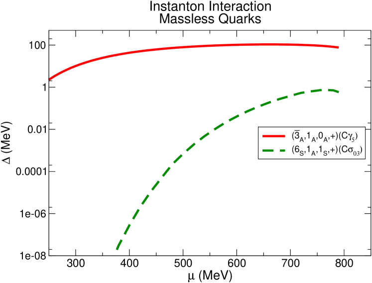
Figure 4.1: Gap parameters in the attractive channels for an NJL interaction based on the two-flavor instanton. Since the instanton interaction requires two quark flavors, we take the quarks to be massless, which is a good approximation for the $u$ and $d$. The cutoff is $\Lambda=800~{}{\rm MeV}$.

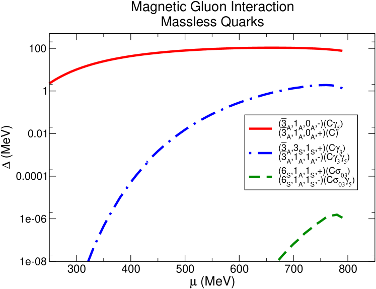
Figure 4.2: Gap parameters in the attractive channels for an NJL interaction based on magnetic-gluon exchange. We show the one-flavor and two-flavor channels, for massless quarks. The cutoff is $\Lambda=800~{}{\rm MeV}$.

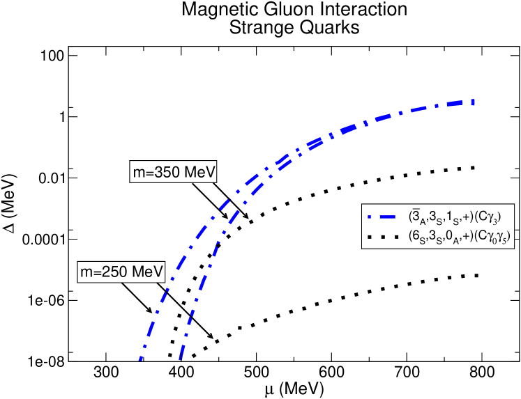
Figure 4.3: Gap parameters in the attractive channels for an NJL interaction based on magnetic-gluon exchange, for quarks of mass 250 and 350 MeV, a reasonable range of values for the strange quark at medium density. We show only the single-flavor channels. The cutoff is $\Lambda=800~{}{\rm MeV}$.

4.3 Gap calculations for the attractive diquark channels

For the attractive channels we performed uncoupled gap equation calculations, and obtained the dependence of the quark pairing on $\mu$. The amount of pairing is given by the gap parameter $\Delta(\mu)$, which occurs in the self energy (See Appendix B.1) as

$$\Delta^{\alpha\beta ab}_{ij}(p)=\Delta(\mu)\,\,{\cal C}^{\rm\alpha\beta}{\cal F}_{ij}\Gamma^{ab}~{},$$ (4.5)

with color matrix ${\cal C}$, flavor matrix ${\cal F}$, and Dirac structure $\Gamma^{ab}$. Note that $\Delta(\mu)$ is a gap parameter, not the gap. It sets the scale of the gap in the quasiparticle excitation spectrum, but as we will see in Section 4.4 the gap itself often depends on the direction of the momentum.

The 4-fermion interactions that we use are nonrenormalizable, so our gap equations (shown explicitly in Appendix B.2) involve a 3-momentum cutoff $\Lambda$, which represents the decoupling of our interactions at higher momentum, due to instanton form factors, effective gluon masses, etc. The usual procedure for NJL model calculations is to calibrate the coupling strength for each cutoff $\Lambda$ by known low-density physics such as the size of the chiral condensate. However, it is well known that this leads to an approximately cutoff-independent maximum gap (as a function of $\mu$) in the $\psi C\gamma_{5}\psi$ channel, so we used that criterion directly as our calibration condition, setting the maximum gap to $100~{}{\rm MeV}$.

The results of our calculations, for cutoff $\Lambda=800~{}{\rm MeV}$, are plotted in Figs. 4.1, 4.2, and 4.3. For other cutoffs the overall shape of the curves is very similar. Because we use a sharp cutoff $\Lambda$, the gap falls to zero when $\mu$ reaches $\Lambda$ (see, e.g., Eq. (B.16)). We show gap plots for the instanton interaction (Fig. 4.1) and magnetic gluon interaction. The full electric + magnetic gluon gives results that are similar to those for the magnetic gluon, but with no gap in the (${\bf 6}_{S}$,${\bf 1}_{A}$,1,+)($C\sigma_{03}$) channel.

For the magnetic gluon, we show a gap plot for massless quarks (Fig. 4.2) which includes the two-flavor channels ($\bar{\bf 3}_{A}$,${\bf 1}_{A}$,0,+)($C\gamma_{5}$), ($\bar{\bf 3}_{A}$,${\bf 1}_{A}$,1,$-$)($C\gamma_{3}\gamma_{5}$) and (${\bf 6}_{S}$,${\bf 1}_{A}$,1,+)($C\sigma_{03}$) which could sustain $u$-$d$ pairing, as well as the single-flavor channel ($\bar{\bf 3}_{A}$,${\bf 3}_{S}$,1,+)($C\gamma_{3}$) which could sustain $u$-$u$ or $d$-$d$ pairing.

We also show a gap plot (Fig. 4.3) for a single quark flavor with mass of 250 or 350 MeV. This is appropriate for the strange quark, whose effective mass is expected to lie between 150 MeV and about 400 MeV (see Ref. [26], Fig. 1).

The relative sizes of the gaps in the different channels reflect the pairing strengths given in Table 4.1. We see that the Lorentz scalar ($\bar{\bf 3}_{A}$,${\bf 1}_{A}$,0,+)($C\gamma_{5}$) (solid line) is dominant. The $j=1$ channels have much smaller gap parameters. The ($\bar{\bf 3}_{A}$,${\bf 3}_{S}$,1,+)($C\gamma_{3}$) gap parameter (dash-dot line in Figs. 4.2 and 4.3) rises to a few MeV with the magnetic gluon interaction. The (${\bf 6}_{S}$,${\bf 1}_{A}$,1,+)($C\sigma_{03}$) gap parameter (dashed line) rises to about 1 MeV with an instanton interaction, but only 1 eV with the magnetic gluon interaction. It should be remembered, however, that the temperature of a compact star can be anything from tens of MeV at the time of the supernova to a few eV after millions of years, so gaps anywhere in this range are of potential phenomenological interest.

The (${\bf 6}_{S}$,${\bf 3}_{S}$,0,+)($C\gamma_{0}\gamma_{5}$) channel (dotted line), which is the only attractive channel for a single color and flavor of quark, is highly suppressed for massless quarks at high density but reaches about 10 keV for strange quarks ($m=350~{}{\rm MeV}$, Fig. 4.3). This is because its particle-particle component goes to zero as $m\to 0$ (Eq. (B.33) and Table 4.1).

Up to this point we have not mentioned the $j=1,m_{j}=\pm 1$ channels (e.g. $\psi C\gamma_{\pm}\psi\equiv\psi C(\gamma_{1}\pm i\gamma_{2})\psi$). We have only discussed the $j=1,m_{j}=0$ channels (e.g. $\psi C\gamma_{3}\psi$). That is because rotational invariance of the interaction Hamiltonian that we are using guarantees that changing $m_{j}$ from 0 to $\pm 1$ will not affect the binding energy and gap equation. This can be seen by considering the form of the binding energy. From Eq. (4.1) it is

$$E_{B}\sim\langle\psi\psi\rangle^{{\dagger}ac}\langle\psi\psi\rangle^{bd}{\cal H}_{abcd}~{}.$$ (4.6)

Note that it is quadratic in the diquark condensate, with one of the factors being complex conjugated. So if we have some 3-vector condensate, for example $\phi=\sum_{i}\phi_{i}\langle\psi\gamma_{i}\psi\rangle$, then its binding energy is

$$E_{B}\propto|\phi_{x}|^{2}+|\phi_{y}|^{2}+|\phi_{z}|^{2}$$ (4.7)

It is clear that the $m_{j}=0$ condensate $\phi_{i}=(0,0,1)$ has the same binding energy as the $m_{j}=\pm 1$ condensate $\phi_{i}=(1/\sqrt{2})(1,\pm i,0)$. We have explicitly solved the gap equations for the $m_{j}=\pm 1$ condensates, and find their solutions identical to the corresponding $m_{j}=0$ condensates. However, the quasiquark excitations in the two cases are quite different, and we proceed to study these in the next section.

4.4 Quasiquark dispersion relations

The physical behavior of quark matter will be dominated by its lowest energy excitations. As well as Goldstone bosons that arise from spontaneous breaking of global symmetries, there will be fermionic excitations of the quarks around the Fermi surface. In the presence of a diquark condensate, the spectrum of quark excitations is radically altered. Instead of arbitrarily low energy degrees of freedom, associated with the promotion of a quark from a state just below the Fermi surface to just above it, there is a minimum excitation energy (gap), above which the excitation spectrum is that of free quasiquarks, which are linear combinations of a particle and a hole.

The dispersion relations of the quasiparticles can be calculated straightforwardly by including a condensate of the desired structure in the inverse propagator $S^{-1}$, shown in Eq. (B.3). Poles in the propagator correspond to zeros in $S^{-1}$, so the dispersion relations are obtained by solving $\det S^{-1}(p_{0},{\mathbf{p}},\mu,\Delta,m)=0$ for the energy $p_{0}$ as a function of the 3-momentum ${\mathbf{p}}$ of the quasiparticle, quark chemical potential $\mu$, gap parameter $\Delta$, and quark mass $m$.

The gap is by definition the energy required to excite the lowest energy quasiquark mode. Isotropic condensates have a uniform gap, but one of the most interesting features of $j>0$ condensates is that they are not in general fully gapped: the gap goes to zero for particular values of momentum ${\mathbf{p}}$, which correspond to particular places on the Fermi surface. This means that transport properties such as viscosities and emissivities, which are suppressed by factors of $\exp(-\Delta/T)$ in phases with isotropic quark pairing, may not be so strongly suppressed by a $j>0$ condensate. In Figs. 4.4 and 4.5 we show the variation of the gap over the Fermi surface by plotting the energy of the lowest excitation as a function of angle,

$$E_{\rm gap}(\theta)=\min_{p,i}|E_{i}(p,\theta)|$$ (4.8)

where $E_{i}(p,\theta)$ is the energy of the $i^{\rm th}$ quasiquark excitation with momentum $(p\sin\theta\cos\phi,p\sin\theta\sin\phi,p\cos\theta)$. For the plots we take $\mu=500~{}{\rm MeV}$ and $\Delta=50~{}{\rm MeV}$, with quark mass $m=0$ (Fig. 4.4) or $m=250~{}{\rm MeV}$ (Fig. 4.5).

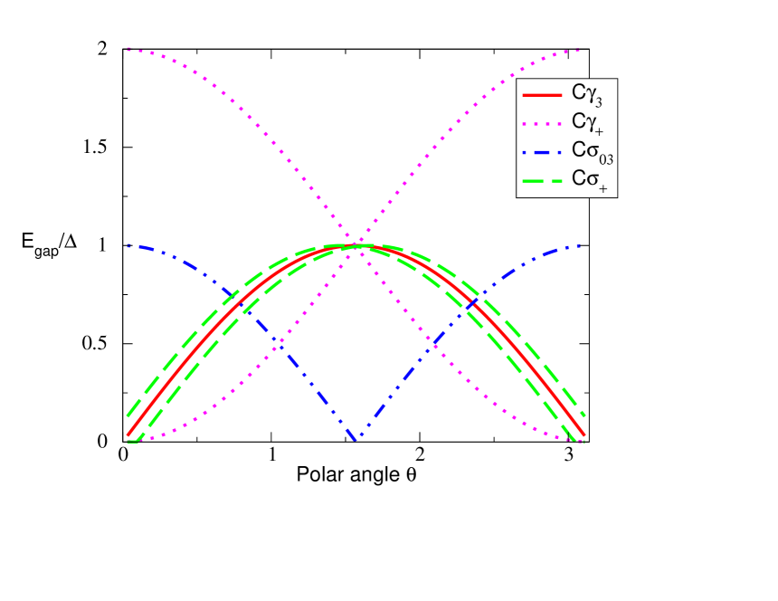
Figure 4.4: Energy gap in units of the gap parameter as a function of polar angle on the Fermi surface for rotational symmetry breaking phases with massless quarks, at $\mu=500~{}{\rm MeV}$, gap parameter $\Delta=50~{}{\rm MeV}$. $\gamma_{+}\equiv\gamma_{1}+i\gamma_{2}$, $\sigma_{+}\equiv\sigma_{01}+i\sigma_{02}$.

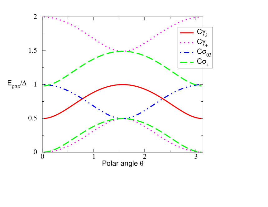
Figure 4.5: Energy gap in units of the gap parameter as a function of polar angle on the Fermi surface for rotational symmetry breaking phases at $\mu=500~{}{\rm MeV}$, with gap parameter $\Delta=50~{}{\rm MeV}$. The quarks have mass $m=250~{}{\rm MeV}$. $\gamma_{+}\equiv\gamma_{1}+i\gamma_{2}$, $\sigma_{+}\equiv\sigma_{01}+i\sigma_{02}$.

• $C\gamma_{3}$ condensate: $j=1,m_{j}=0$.
  There is one quasiquark excitation with energy less than the gap parameter $\Delta$.

  $$\begin{array}[]{rcl}E(p)^{2}&=&(\sqrt{p^{2}+m^{2}\mu^{2}/\mu_{\rm eff}^{2}}\pm\mu_{\rm eff})^{2}+\Delta_{\rm eff}^{2}\\[4.30554pt] \mu_{\rm eff}(\theta)^{2}&=&\mu^{2}+\Delta^{2}\cos^{2}(\theta)\\[4.30554pt] \Delta_{\rm eff}(\theta)^{2}&=&\Delta^{2}\Bigl{(}\sin^{2}(\theta)+m^{2}/\mu_{\rm eff}^{2}\cos^{2}(\theta)\Bigr{)}\end{array}$$ (4.9)

  From the expression for $\Delta_{\rm eff}(\theta)$ we see that for massless quarks the gap goes to zero for momenta parallel to the $z$-axis, i.e. at the poles on the Fermi surface (solid curve in Fig. 4.4). Massive quarks retain a small gap of order $m\Delta/\mu$ at the poles (solid curve in Fig. 4.5).

• $C(\gamma_{1}\pm i\gamma_{2})$ condensate: $j=1,m_{j}=\pm 1$.
  There are two quasiquark excitations with energy less than $2\Delta$,

  $$\begin{array}[]{rl}E(p)^{2}=2\Delta^{2}+m^{2}+\mu^{2}+p^{2}\pm&\Bigl{(}4\Delta^{4}+4\mu^{2}(p^{2}+m^{2})+2\Delta^{2}p^{2}(1-\cos(2\theta))\\ &\pm 4\Delta^{2}\mu\sqrt{4m^{2}+2p^{2}(1+\cos(2\theta))}\Bigr{)}^{\textstyle\frac{1}{2}}\end{array}$$ (4.10)

  For this condensate the effective gap again goes to zero at the poles, but in this case it remains zero even in the presence of a quark mass (dotted curve in Figs. 4.4,4.5).

• $C\sigma_{03}$ condensate: $j=1,m_{j}=0$.
  There is one quasiquark excitation with energy less than $\Delta$, its dispersion relation is [98]

  $$\begin{array}[]{rcl}E(p)^{2}&=&(\sqrt{p^{2}+m^{2}\mu^{2}/\mu_{\rm eff}^{2}}\pm\mu_{\rm eff})^{2}+\Delta_{\rm eff}^{2}\\[4.30554pt] \mu_{\rm eff}(\theta)^{2}&=&\mu^{2}+\Delta^{2}\sin^{2}(\theta)\\[4.30554pt] \Delta_{\rm eff}(\theta)^{2}&=&\Delta^{2}\Bigl{(}\cos^{2}(\theta)+m^{2}/\mu_{\rm eff}^{2}\sin^{2}(\theta)\Bigr{)}\end{array}$$ (4.11)

  This is related to the dispersion relation for the $C\gamma_{3}$ condensate by $\theta\to\pi/2-\theta$: for massless quarks the quasiquarks are gapless around the equator of the Fermi sphere (dash-double-dot curve in Fig. 4.4) and in the presence of a quark mass they gain a small gap of order $\Delta m/\mu$ (dash-double-dot curve in Fig. 4.5). The equator is a larger proportion of the Fermi surface than the poles, so in this case we might expect a greater effect on transport properties.

• $C(\sigma_{01}\pm i\sigma_{02})$ condensate: $j=1,m_{j}=\pm 1$.
  There are two quasiquark excitations with energy less than $\Delta$. They have rather complicated dispersion relations. Going to the massless case, and assuming $E,(p-\mu)\ll\mu$, which will be true for the low-energy quasiquark degrees of freedom that we are interested in, we find

  $$\begin{array}[]{rcl}E(p)&=&(\Delta^{2}\mu+\Delta^{2}p\cos(\theta)\pm\eta/\sqrt{2})/(2\mu^{2})\\ \eta^{2}&=&(8\mu^{4}(\mu-p)^{2}+8\Delta^{2}\mu^{2}(\mu^{2}-\cos(\theta)^{2}p^{2})+2\Delta^{4}(\mu+\cos(\theta)p)^{2})\end{array}$$ (4.12)

  In this case there is a region near the poles, $\theta\lesssim\Delta/\mu$, where the gap is zero (dashed curve in Fig. 4.4). This is because at those angles $E(p)$ has zeros at two values of $p$ close to $\mu$. When $\theta\approx\Delta/\mu$ those two zeros merge and disappear from the real $p$ axis. The presence of a quark mass $m>\Delta$ wipes out this effect, but there is still no gap at the poles on the Fermi surface (dashed curve in Fig. 4.5).

In comparing Figs. 4.4 and 4.5 it is interesting to note that introducing a mass for the quark opens up a gap whenever the gap lines intersect each other at a non-zero angle (after one includes the mirror-image negative-energy gap curves for the quasiholes). This occurs at zero energy at the poles for $C\gamma_{3}$ and at the equator for $C\sigma_{03}$. It occurs at non-zero energy for $C(\gamma_{1}\pm i\gamma_{2})$. The case of $C(\sigma_{01}\pm i\sigma_{02})$ is similar, but it is not obvious from the gap plot for reasons described above.

We see that the $j\neq 0$ phases show a rich variety of quasiquark dispersion relations. For massless quarks they are all gapless in special regions of the Fermi surface, and for massive quarks the $m_{j}=\pm 1$ condensates remain gapless for momenta parallel to the spin. It follows that for these phases the quasiquark excitations will play an important role in transport properties, even when the temperature is less than the gap parameter.

Moreover, different condensates ($m_{j}=\pm 1$ vs. $m_{j}=0$) that because of rotational invariance of the Hamiltonian have exactly the same binding energy and gap equation, nevertheless have completely different energy gaps over the Fermi surface. They will therefore behave quite differently when exposed to nonisotropic external influences, such as magnetic fields or neutrino fluxes, and also in their coupling to external sources of torque, e.g. via electron-quasiquark scattering. All these influences are present in compact stars, and it will be interesting and complicated to sort out which is favored under naturally occurring conditions. And it should not be forgotten that these conditions vary with the age of the star.

4.5 Conclusions

In this chapter we have completed a mean-field survey of 24 different channels for diquark condensation, using an NJL model with Fermi couplings for instantons and pointlike gluons. Our catalog of channels is by no means comprehensive, but it does exhaust the possibilities for structures that can be factorized into separate tensors for color, flavor, and spin (notably, this excludes interesting “locking” phases such as color-flavor-locking or color-spin-locking).

As we promised in section 4.1, we can identify single-color and/or single-flavor phases that are useful for pairing “orphaned” quarks in the various pairing scenarios described at the start of this chapter. In fact our survey reveals five channels that are attractive and therefore susceptible to BCS condensation in the NJL model. In the same order that they are listed in table 1.1, these channels are:

2SC	($\bar{\bf 3}_{A}$,${\bf 1}_{A}$,0,$+$)($C\gamma_{5}$)
spin-one 2SC	($\bar{\bf 3}_{A}$,${\bf 1}_{A}$,1,$-$)($C\gamma_{3}\gamma_{5}$)
single-color	(${\bf 6}_{S}$,${\bf 1}_{A}$,1,+)($C\sigma_{03}$)
single-flavor	($\bar{\bf 3}_{A}$,${\bf 3}_{S}$,1,$+$)($C\gamma_{3}$)
single-color and single-flavor	(${\bf 6}_{S}$,${\bf 3}_{S}$,0,$+$)($C\gamma_{0}\gamma_{5}$)

The first is well-known, the second is an obscure (and never-favored) spin-one cousin of the 2SC phase, and the last three are the channels that are good for pairing orphaned quarks. For these attractive channels we have calculated gaps and the results are shown in Figs. 4.1, 4.2, and 4.3. (Note that Fig. 4.2 also shows two more channels which are parity-partners of the 2SC and single-color channels. These channels are attractive for gluons, but they are parity odd and disfavored by instantons.)

The gap of the 2SC phase has been calculated, by various methods, to be in the range of 10 to 100 MeV. In the present work we have assumed a maximum 2SC gap of 100 MeV and used this assumption to calibrate the NJL models. Then we find, as shown in Figs. 4.1, 4.2, and 4.3, that the “exotic” phases have gaps that are no larger than about 1 MeV and can be orders of magnitude smaller than this. Notice that while the 2SC gap curve is fairly flat on these plots, the gap curves for the exotic phases are quite steep. Because these are semilog plots this implies that the exotic gaps are drastically $\mu$-dependent. They can change by more than two orders of magnitude when the chemical potential is increased from 400 MeV to 500 MeV.

Moreover, the gap values are very sensitive to the choice of NJL model. For example, the gap for the single-color phase is seen to differ by six orders of magnitude when it is calculated with an instanton interaction (dashed line in Fig. 4.1) versus a magnetic gluon interaction (dashed line in Fig. 4.2). In both cases the NJL model is calibrated to give the same value (100 MeV) for the 2SC gap. Both the instanton and magnetic gluon interactions are reasonable models for some physics at moderate densities, but they yield very different results for the gap in this single-color phase.

Buballa et al [98] observed similar difficulties in their NJL investigation of the single-color state. The model uncertainties cannot be resolved by appealing to a perturbative calculation at asymptotically high densities, because the long-range magnetic gluon which dominates at these densities [12] is always repulsive in the color-symmetric channel [63] and therefore does not predict a single-color pairing state.

The calculation for the single-flavor phase is also very model-sensitive. However, in this case the state can be studied with a perturbative, model-independent calculation in the high density limit [63, 64]. In this regime we find the simple result that the spin-one (single-flavor) gap is $\Delta=c\Delta_{0}$, where $\Delta_{0}$ is the spin-zero (2SC) gap and $c$ a constant (independent of $\mu$) that is somewhere between 0.002 and 0.01 (the constant is known exactly and depends on the particular spin ansatz, e.g. polar phase or color-spin-locking phase). The spin-one gap therefore varies less drastically with $\mu$ than in NJL models because it is just a constant fraction of the spin-zero gap. If we assume (without justification) that this relation holds at moderate densities, we predict a spin-one gap of 200 keV to 1 MeV, for a spin-one gap of 100 MeV. For $\mu$ of 400 to 500 MeV, the NJL calculation predicts a much smaller gap that ranges from 0.1 to 10 keV in this $\mu$ interval.

In the high-density limit, the single-flavor condensate also includes an admixture of the $C\sigma_{03}$ spin channel. This channel is repulsive in the NJL model but attractive for long-range magnetic gluons. In the high-density limit the color structure alone dictates the attractiveness of the pairing channel: color-symmetric pairing is repulsive and color-antisymmetric pairing is attractive, independent of color or spin [63]. But this simple conclusion is unlikely to persist at moderate densities when various in-medium effective interactions (like those of our NJL model) can supersede this perturbative result.

The preceding discussion is intended to convey that our NJL calculations should be interpreted conservatively. They are useful because they indicate which pairing channels are most likely to be attractive at moderate densities that are of interest to us. But they provide only very rough estimates for the magnitudes of the gaps in the various channels. In our summary of pairing channels shown in table 1.1, we have estimated rough upper limits for the gaps by taking the peak values of these gaps from figures Figs. 4.1, 4.2, and 4.3. These numbers should be interpreted as reasonable upper bounds for gaps which could be orders of magnitude smaller.

Although many of the channels we have studied have very small gaps and therefore very small critical temperatures, they will be phenomenologically relevant if they are the best pairing option available for some of the quarks. Since the temperature of a compact star falls to tens of eV when its age reaches millions of years, pairing can occur in such channels late in the star’s life. The corresponding quasiquark excitations will become massive and this can suppress their participation in transport processes. With this in mind it would be useful to extend our analysis of the exotic condensates to finite temperature. Recent work indicates that the usual BCS relationship between the critical temperature and the gap parameter may be modified for spin-one condensates [98, 64].

The spin-one condensates are gapless at special 3-momenta (or nearly so with nonzero quark masses). Recall that the $(j=1,m_{j}=\pm 1)$ condensates ($\psi C(\gamma_{1}\pm i\gamma_{2})\psi$ or $\psi C(\sigma_{01}\pm i\sigma_{02})\psi$) always have gapless quasiquarks at the poles of the Fermi sphere. The $j=1,m_{j}=0$ condensates have gapless regions for massless quarks, at the poles ($\psi C\gamma_{3}\psi$) or around the equator ($\psi C\sigma_{03}\psi$), but if the quarks are massive then the quasiquarks have a minimum gap of order $m\Delta/\mu$ (Figs. 4.4, 4.5). The gapless or nearly gapless modes may continue to play a role in transport processes, even when the temperature is much less than the gap parameter. It would be very useful to develop a transport theory for the spin-one condensates, to determine how the light modes contribute to neutrino emission/absorption via URCA processes or otherwise, and how they affect specific heat, viscosity, conductivities, etc. A natural first step would be to write down an effective theory, which would contain the lowest quasiquark modes and Goldstone bosons arising from the breaking of rotational symmetry (which could be called “spin waves” by analogy with helium-3 [97]).

If spin-one color condensates occur in compact stars, they are likely to have interesting and complicated spatial and rotational textures like those of the various spin-one helium-3 phases. The $j=1$ condensates can carry angular momentum simply by aligning themselves in large domains, without involving any superfluid vortices, but it seems they will typically occur in conjunction with other phases that are superfluid. It would be interesting to investigate how the angular momentum is carried in this situation.

Finally, we note that since the single-flavor color superconductor has a small gap and also exhibits an electromagnetic Meissner effect [96] (unlike the CFL phase [59]), it could have an upper critical magnetic field smaller than that of some pulsars. We can estimate the critical field by assuming that the critical magnetic energy density is comparable to the condensation energy of the color superconductor, i.e. $B_{c}^{2}/8\pi\sim\mu^{2}\Delta^{2}/\pi^{2}$. By this estimate, pulsars with typical fields of $10^{12}-10^{13}$ Gauss could destroy single-flavor pairing if the gap is smaller than $0.1-1$ keV, and magnetars with fields of order $10^{15}-10^{16}$ Gauss could destroy condensates with gaps of as large as $0.1-1$ MeV.

blah

Chapter 5 Applications and Outlook

5.1 Overview

In this final chapter we take a closer look at two physical settings in which the crystalline phase might occur with observable consequences. The first setting is astrophysical: the quark matter core of a rotating compact star, where a layer of crystalline quark matter can pin vortices and cause glitches. The second setting is terrestrial: an ultracold trapped gas of fermionic atoms, where a spin imbalance can induce the formation of a crystalline superfluid. In the last section, we close by describing unsolved problems and directions for future research.

5.2 Pulsar glitches

Many pulsars have been observed to glitch. Glitches are sudden jumps in rotation frequency $\Omega$ which may be as large as $\Delta\Omega/\Omega\sim 10^{-6}$, but may also be several orders of magnitude smaller. The frequency of observed glitches is statistically consistent with the hypothesis that all radio pulsars experience glitches [115]. Glitches are thought to originate from interactions between the rigid crust, somewhat more than a kilometer thick in a typical neutron star, and rotational vortices in the neutron superfluid. The inner kilometer of the crust consists of a rigid lattice of nuclei immersed in a neutron superfluid [116]. Because the pulsar is spinning, the neutron superfluid (both within the inner crust and deeper inside the star) is threaded with a regular array of rotational vortices. As the pulsar’s spin gradually slows due to emission of electromagnetic radiation, these vortices must gradually move outwards since the rotation frequency of a superfluid is proportional to the density of vortices. Deep within the star, the vortices are free to move outwards. In the crust, however, the vortices are pinned by their interaction with the nuclear lattice. What happens next varies from model to model. Perhaps the vortices exert sufficient force on the crust to tear it apart, resulting in a sudden breaking and rearrangement of the crust and a change in the moment of inertia [117]. Perhaps a large cluster of vortices within the inner crust builds up enough outward pressure to overcome the pinning force, suddenly becomes unpinned, and moves macroscopically outward [118, 119, 120, 121, 122, 123, 124]. This sudden decrease in the angular momentum of the superfluid within the crust results in a sudden increase in angular momentum of the rigid crust itself, and hence a glitch. Perhaps, due to interactions between neutron vortices and proton flux tubes, the neutron vortices pile up just inside the inner crust before suddenly coming unpinned [125]. Although the models differ in important respects, all agree that the fundamental requirements are the presence of rotational vortices in a superfluid, and the presence of a rigid structure which impedes the motion of these vortices (by a pinning force of suitable magnitude) and which encompasses enough of the volume of the pulsar to contribute significantly to the total moment of inertia.

Although it is premature to draw quantitative conclusions, it is interesting to speculate that some glitches may originate not at the crust, but deep within a pulsar which has a color superconducting quark matter core. If some region of the core is in the crystalline phase, because this phase is a superfluid it will be threaded by an array of rotational vortices, and these vortices may be pinned in the crystal by the periodic spatial modulation of the diquark condensate. The basic reasoning is that because the diquark condensate must vanish in the core of a rotational vortex, the vortex might prefer to reside at at a node of the LOFF crystal. It is interesting to note that enhanced pinning of magnetic flux tubes has been proposed as an experimental signature of the LOFF phase in an electron superconductor [127]. (However, the analogy may be misleading, because the underlying pinning mechanisms may differ for quark matter versus electrons in a solid, as we will discuss.)

Before we delve into an assessment of the feasibility of quark matter glitching, it is worth noting that perhaps the most interesting consequence is for compact stars made entirely of quark matter (also commonly called “strange quark matter” because it will contain strange quarks in addition to up and down quarks). The work of Witten [128] and Farhi and Jaffe [129] suggests that strange quark matter may be energetically stable relative to nuclear matter even at zero pressure. Then it might occur that observed compact stars are strange quark stars [130, 131] rather than neutron stars. This has recently been suggested for certain accreting compact stars [132], although the evidence is far from unambiguous [133]. A conventional neutron star may feature a core made of strange quark matter, but strange quark stars are made (almost) entirely of quark matter with either no hadronic matter content at all or with a thin crust, of order one hundred meters thick, which contains no neutron superfluid [131, 137] (the nuclei in this thin crust are supported above the quark matter by electrostatic forces; these forces cannot support a neutron fluid). Because of the absence of superfluid neutrons, and because of the thinness of the crust, no successful models of glitches in the crust of a strange quark star have been proposed. Since pulsars are observed to glitch, the apparent lack of a glitch mechanism for strange quark stars has been the strongest argument that pulsars cannot be strange quark stars [138, 139, 140]. This conclusion must now be revisited: the quark matter in a strange star would be a color superconductor, and glitches may originate from pinning of vortices within a layer of the strange star which is in a crystalline color superconducting state.

Crystalline quark matter glitching is more interesting for strange stars than for other compact stars, because it is the only way for strange stars to glitch. Certainly, crystalline quark matter glitching could also occur in a more conventional neutron star with a quark matter core, but the core would be one of two potential locations where glitches may originate. Any attempt to observe a quark matter glitch would therefore require glitching models that are sophisticated enough to enable differentiation between the signatures of a quark matter core glitch and a nuclear matter crustal glitch.

In this context the reader may be concerned that a glitch deep within the quark matter core of a neutron star may not be observable. However, due to electron scattering off vortices, the rotation of the superfluid interior of the star is coupled to the rotation of the electron plasma on a very short time scale (on the order of seconds), and the rotation of the electron plasma is subsequently coupled to the rotation of the outer crust on a similarly short time scale. Therefore the crust will rapidly respond to a change in the rotation of the interior superfluid [142]. This rapid coupling of the superfluid to the crust, due to the fact that the electron plasma penetrates throughout the star, is usually invoked to explain that the core nucleon superfluid speeds up quickly after a crustal glitch: the only long relaxation time is that of the vortices within the inner crust. Here, we invoke it to explain that the crust speeds up rapidly after a core glitch has accelerated the superfluid just outside the LOFF layer. After a glitch in the LOFF region, the only long relaxation times are those of the vortices in the LOFF region and in the inner crust.

Our proposed quark matter glitch mechanism requires that the crystalline color superconducting phase occupies enough of the interior of a compact star to appreciably contribute to the star’s moment of inertia. To address this question we need to complete a realistic three-flavor analysis of the crystalline state, and map out the $\mu$ interval that the crystalline state will occupy in the real QCD phase diagram (figure 1.1). The extent of this interval will determine the extent of any volume of crystalline color superconductivity inside a compact star. So far, of course, we have only studied the crystalline state in a two-flavor model. In this model, we saw that the plane wave crystalline state is favored only when ${\delta\mu}/\Delta_{0}$ is in a small interval $[{\delta\mu}_{1}/\Delta_{0},{\delta\mu}_{2}/\Delta_{0}]\approx[0.707,0.754]$ (where $\Delta_{0}$ is the gap in the homogeneous BCS phase, i.e. 2SC), but when we extended our analysis to multiple plane wave crystals we found that the crystalline phase could occur over a much larger interval $[{\delta\mu}_{1}^{\prime}/\Delta_{0},{\delta\mu}_{*}/\Delta_{0}]$ (as sketched in figure 1.4). Extending the analysis to three flavors, we expect that the ${\delta\mu}/\Delta_{0}$ interval of the two-flavor problem will correspond to an interval of $m_{s}^{2}/4\mu\Delta_{0}$ in the three-flavor problem. If the plane wave crystal were favored, it would only occupy a small sliver in the QCD phase diagram. The much more robust FCC crystal can occupy a much larger region, perhaps even the entire interval between the hadronization and unlocking transitions. As a function of increasing depth in a compact star, $\mu$ increases, $m_{s}$ decreases, and $\Delta_{0}$ also changes, and the crystalline phase will occur wherever $m_{s}^{2}/4\mu\Delta_{0}$ is in the (large) interval where the crystalline phase is favored. Therefore while a quantitative analysis is yet to be done, we have reason to believe that the crystalline phase could encompass a significant volume of the quark matter core of a compact star.

The next issue to resolve is whether the crystalline phase will actually pin vortices. A real demonstration of pinning, and a real calculation of the pinning force, will require explicitly constructing a vortex in the crystalline phase, and then observing how the energy of the vortex varies as it is moved across the crystal. As we shall discuss below, however, it is difficult to construct a vortex solution on top of the existing modulation of the crystalline condensate. The difficulty is related to the fact that the vortex is itself a deformation of the crystal, because both vortex and crystal are made of the same diquark condensate. It is easier to understand pinning in the nuclear crust, because there are two components involved: the first component (the lattice of nuclei) is a substrate that causes pinning in the second component (the neutron superfluid). It is the spatial variation of the substrate that pins superfluid vortices, not a crystalline variation of the superfluid order parameter itself. In other words, the superfluid does not “self-pin”. In an electron superconductor, magnetic flux tubes are pinned to a substrate of random magnetic impurities. Enhancement of pinning in an electronic LOFF phase could occur by self-pinning of the LOFF crystal; however, an alternative proposal is that the the LOFF phase does not self-pin but just makes it easier for the magnetic flux tubes to be pinned by the magnetic impurities. There is no “substrate” underlying quark matter, so if pinning does occur in the crystalline color superconductor, it must occur by self-pinning of superfluid vortices by the crystalline modulation of the same superfluid.

Supposing that there is pinning, we can make an order-of-magnitude estimate of the pinning force which sidesteps the complications involved in explicitly constructing a vortex solution (at the end of this section we will return to the vortex problem and discuss some preliminary investigations). We perform a calculation similar to that done by Anderson and Itoh [118] for the pinning of neutron vortices in the inner crust of a neutron star. In that context, the pinning calculation has since been made quantitative [145, 122, 124]. We will attempt an estimate for both the plane wave LOFF phase and the more robust multiple-plane wave state (i.e. the FCC crystal). For the former, we can use numbers for the gap and free energy as in Figure 2.4. That is, we assume that at $\bar{\mu}=400\ \mbox{MeV}$ we have a BCS gap $\Delta_{0}=40\ \mbox{MeV}$ and a BCS free energy of $\Omega_{0}=2.6\times 10^{7}\ \mbox{MeV}^{4}$ at ${\delta\mu}=0$; then at ${\delta\mu}_{1}$ the gap for the plane-wave LOFF state is $\Delta_{\mbox{\scriptsize pw}}\simeq 8\ \mbox{MeV}\simeq 0.2\Delta_{0}$ and the phase is favored over the normal state by a free energy $\Omega_{\mbox{\scriptsize pw}}\simeq 5\times 10^{4}\ \mbox{MeV}^{4}$. The periodicity of the crystal is $b_{\mbox{\scriptsize pw}}=\pi/(2|{\mathbf{q}}|)\simeq 9$ fm, and the thickness of a rotational vortex is given by the correlation length $\xi_{\mbox{\scriptsize pw}}\sim 1/\Delta_{\mbox{\scriptsize pw}}\sim 25$ fm. For the FCC state, we cannot yet calculate numbers for the gap and free energy but we will use $\Delta_{\mbox{\scriptsize fcc}}\sim\Delta_{0}/2=20\ \mbox{MeV}$ and $\Omega_{\mbox{\scriptsize fcc}}\sim\Omega_{\mbox{\scriptsize BCS}}/4=6.5\times 10^{6}\ \mbox{MeV}^{4}$, reflecting our prediction that the FCC phase is robust. The node spacing is $b_{\mbox{\scriptsize fcc}}=\sqrt{3}\pi/(2|{\mathbf{q}}|)\simeq 15$ fm (i.e. half the lattice constant, equation (1.26)), and the thickness of a rotational vortex is $\xi_{\mbox{\scriptsize fcc}}\sim 1/\Delta_{\mbox{\scriptsize fcc}}\sim 10$ fm. All these numbers are quite uncertain, but we will use them for the present. In the context of crustal neutron superfluid vortices, there are three distinct length scales: the vortex thickness $\xi$, the lattice spacing between nuclei $b$, and $R$, the radius of the individual nuclei. (The condensate vanishes within regions of size $R$ separated by spacing $b$.) In the LOFF phase, the latter two length scales are comparable: since the condensate varies like a sum of plane waves it is as if $R\sim b$. The fact that these length scales are similar in the LOFF phase will complicate a quantitative calculation of the pinning energy; it makes our order of magnitude estimation easier, however. The pinning energy is the difference between the energy of a section of vortex of length $b$ which is centered on a node of the LOFF crystal versus one which is centered on a maximum of the LOFF crystal. It is of order

$$E_{p}\sim\Omega b^{3}\sim\left\{\begin{array}[]{ll}4\ \mbox{MeV}\phantom{blah}&\mbox{plane wave}\\ 3\ \mbox{GeV}&\mbox{FCC crystal}\end{array}\right.$$ (5.1)

The resulting pinning force per unit length of vortex is of order

$$f_{p}\sim\frac{E_{p}}{b^{2}}\sim\left\{\begin{array}[]{ll}(5\ \mbox{MeV})/(100\ \mbox{fm}^{2})\phantom{blah}&\mbox{plane wave}\\ (1\ \mbox{GeV})/(100\ \mbox{fm}^{2})&\mbox{FCC crystal}\end{array}\right.$$ (5.2)

The fact that $b$ and $\xi$ are comparable length scales will make a complete pinning force calculation more difficult and is likely to yield an $f_{p}$ which is significantly less than that we have obtained by dimensional analysis [122, 124]. Therefore these figures should be interpreted as upper-bound estimates. Note that our estimate of $f_{p}$ is quite uncertain both because it is only based on dimensional analysis and because the values of $\Delta$, $b$ and $\Omega$ are known to only within an order of magnitude at best. For comparison, we present the corresponding numbers for the pinning of crustal neutron vortices: the pinning energy of neutron vortices in the inner crust is [122]

$$E_{p}\approx 1-3{\rm\ MeV}$$ (5.3)

and the pinning force per unit length is [122, 123]

$$f_{p}\sim\frac{E_{p}}{b\xi}\approx\frac{1-3{\rm~{}MeV}}{(25-50{\rm~{}fm})(4-20{\rm~{}fm})}\ ,$$ (5.4)

where the form of this expression is appropriate because $\xi<b$. Of course it is premature to compare our crude results (5.1, 5.2) for quark matter pinning to the results (5.3, 5.4) of serious calculations for the pinning of crustal neutron vortices as in Refs. [145, 122, 124]. Nevertheless, we observe that the results are comparable for the case of a plane wave LOFF state, while pinning in the more robust FCC state could be orders of magnitude stronger than nuclear pinning (again, however, we are likely overestimating the pinning force so the numbers should be interpreted as upper bounds).

The nuclear pinning force (5.4), when applied in a stellar model, does yield crustal glitches in accord with those observed in pulsars. It remains to be seen whether a much stronger pinning force, occurring in a crystalline region of the quark matter core, would also yield glitches consistent with observation. If the pinning force is large, then the restraint of vortices could be limited by the critical shear stress of the crystal: if the critical shear stress is exceeded, then the vortex can be released by a crystal dislocation. A dimensional analysis, like that which we have done for the pinning force, can only predict that the pinning force and the critical shear stress are of comparable magnitude, and no conclusion can be reached without a more careful investigation.

We now return to the problem of constructing a vortex in the crystalline phase. Vortices are usually constructed beginning with a Ginzburg-Landau free energy functional written in terms of $\Delta({\mathbf{x}})$ and $\boldsymbol{\nabla}\Delta({\mathbf{x}})$. Instead, we have constructed a Ginzburg-Landau potential (equation 3.24) that is written in terms of the momentum modes $\Delta_{\mathbf{q}}$ of the order parameter . In principle, this contains the same information, but it is not well-suited to the analysis of a localized object like a vortex. In position space, the Ginzburg-Landau free energy should look like

$$\Omega[\Delta({\mathbf{x}})]=\Delta({\mathbf{x}})^{*}\left[\alpha+C(\nabla^{2}+4q_{0}^{2})^{2}\right]\Delta({\mathbf{x}})+\mathcal{O}(\Delta^{4})$$ (5.5)

where $C$ is a positive constant and $\alpha$ is the same parameter that appears in equation (3.24), i.e. it is negative below the second-order point ${\delta\mu}_{2}$. The quadratic term successfully reproduces the plane-wave instability of the LOFF phase: just below the second-order point, all the modes on the sphere $|{\mathbf{q}}|=q_{0}$ become unstable. Adding quartic and higher terms to equation (5.5) is difficult, however, because these terms are Fourier transforms of the complicated $J$ and $K$ functions defined in chapter 3. Terms with high powers of spatial derivatives will be required to reproduce the effects of $J$ and $K$ and somehow yield a functional that is minimized by an FCC crystal (equation 1.25). So it is not at all clear that the usual methodology for constructing a vortex starting from a position-space Ginzburg-Landau potential is the right approach.

As always, it should be easier to understand the physics of a vortex far from its core. The natural expectation is that far from its core, a vortex will be described simply by multiplying the $\Delta({\mathbf{x}})$ of (1.25) by $\exp[i\theta({\mathbf{x}})]$, where $\theta({\mathbf{x}})$ is a slowly varying function of ${\mathbf{x}}$ that winds once from 0 to $2\pi$ as you follow a loop encircling the vortex at a large distance. In a uniform superfluid, this slowly varying phase describes a particle-number current flowing around the vortex. But in the crystal, the resulting particle-number current is

$$\mathbf{J}=(\boldsymbol{\nabla}\theta({\mathbf{x}}))|\Delta({\mathbf{x}})|^{2}$$ (5.6)

and the current does not flow in a large loop because it vanishes at the nodal planes of the crystal (see figure 1.6). The dilemma is that the FCC crystal structure divides all of space into small cells bounded by intersecting nodal planes, and a supercurrent cannot flow across a nodal plane. In the presence of a vortex, the crystal structure must change to accommodate the rotational supercurrent flow.

One obvious possibility is that the condensate just reduces to a one-dimensional standing wave $\cos(2{\mathbf{q}}\cdot{\mathbf{x}})$ with no variation in the transverse direction. This condensate is just a stack of layers separated by nodal planes perpendicular to ${\mathbf{q}}$, and vorticity is easily achieved (the supercurrent just circulates in each transverse layer). If this is what happens, then the vortices will not be pinned because they can move freely in the transverse directions.

However, it may not be necessary to change the crystal structure so drastically. Suppose we instead consider changing the different $\Delta_{{\mathbf{q}}}$’s by small phases, i.e. we consider condensates of the form

$$\Delta({\mathbf{x}})=\sum_{{\mathbf{q}}}\Delta_{\mathbf{q}}e^{i2{\mathbf{q}}\cdot{\mathbf{x}}}=\sum_{{\mathbf{q}}}\Delta e^{i\phi_{q}}e^{i2{\mathbf{q}}\cdot{\mathbf{x}}}$$ (5.7)

(we assume that all the $\Delta_{\mathbf{q}}$’s keep the same magnitude $\Delta$). These are small distortions of the FCC ground state but perhaps these small distortions can change the nodal structure to accommodate vortices. For small phases, we can expand the free energy quadratically:

$$\Omega(\{\phi_{\mathbf{q}}\})=\Omega_{0}+\sum_{{\mathbf{q}},{\mathbf{q}}^{\prime}}\phi_{\mathbf{q}}M_{{\mathbf{q}}{\mathbf{q}}^{\prime}}\phi_{{\mathbf{q}}^{\prime}}+\mathcal{O}(\phi^{4})$$ (5.8)

Odd powers of $\phi$ are not allowed because the free energy should be symmetric under $\Delta({\mathbf{x}})\rightarrow\Delta({\mathbf{x}})^{*}$. The matrix $M$ can be diagonalized to find eight normal modes for the phase angles. Four of these normal modes will have zero eigenvalue. One mode is a common phase for all eight ${\mathbf{q}}$’s (i.e. the superfluid mode). Recalling that the eight ${\mathbf{q}}$’s correspond to eight corners of a cube, the other three zero modes assign a common phase $e^{i\varphi}$ to the four corners of one face of the cube, and an opposite phase $e^{-i\varphi}$ to the four corners of the opposite face. These are the three phonon zero modes; they correspond to translations in the $x$, $y$, or $z$ directions by a displacement $\sqrt{3}\varphi/(2|{\mathbf{q}}|)$. There is one nonzero “tetrahedral” mode which assigns a common phase to four tetrahedral corners of the cube (i.e. four nonadjacent corners) and the opposite phase to the other four corners. Finally, there are three “skew” modes which have the same nonzero eigenvalue of $M$; these modes assign a common phase to the four corners that are the endpoints of two opposite edges of the cube, and an opposite phase to the other four corners.

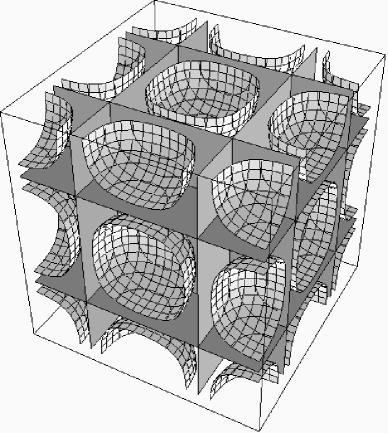
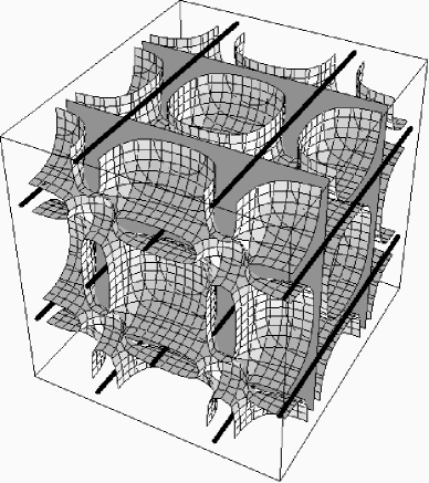
Figure 5.1: The effect of distorting the crystal by a phase shift, as in equation (5.7). On the left is the FCC crystal (phase shift 0); on the right is the distorted crystal (with a “skew” phase shift of magnitude $\pi/8$). The gap function $\Delta({\mathbf{x}})$ vanishes on the gray nodal planes and on the heavy black nodal lines. The curved surfaces are contours where $|\Delta({\mathbf{x}})|=2.6\Delta$ (note that for the undistorted crystal, $|\Delta({\mathbf{x}})|$ is simple cubic even though $\Delta({\mathbf{x}})$ is FCC).

It is these last three “skew” modes that might be of interest. In figure 5.1 we see what happens to the crystal if a small phase is applied for one of these modes. The result is that only one set of parallel nodal planes remains, while the other nodal planes vanish and are replaced by nodal lines. With this deformation it should be possible to have circulating supercurrents in the layers between the remaining nodal planes, and the cost of the nodal deformation that accommodates this vorticity is small when the skew phase angle is small. Moreover, there is still a transverse variation of the condensate, and this could cause vortex pinning. In particular, the vortices might pin at the new nodal lines. In the deformed crystal, a current can be turned on by letting the different $\Delta_{\mathbf{q}}$’s have different magnitudes. The next step is to slowly vary these magnitudes so that the current circulates in a large loop. This investigation is proceeding at the time of this writing.

5.3 Ultracold Fermi gases

One of the most exciting prospects of the LOFF crystalline phase is the possibility that it could be observed as a “crystalline superfluid” in a trap of ultracold fermionic atoms [106]. This could provide a laboratory test of our prediction that the LOFF phase has an FCC crystal structure. Even more significantly, the LOFF phase should be of interest to experimenters because it might in fact be easier to observe than the uniform phase: while the onset of uniform BCS superfluidity in the atomic system could be subtle to detect [146], the onset of crystallization could have a dramatic observational signature. Indeed, it might be possible to literally see the crystal structure, as we will discuss.

In section 1.7.2, we described how the two-flavor NJL model that we have used to investigate the crystalline color superconducting phase might be a surprisingly good model for the analysis of LOFF pairing in an atomic system. This is why we expect our prediction of an FCC crystal structure to apply in the atomic context. In this context, the two species that pair are the two hyperfine states of the fermionic isotope that is being trapped (experimenters have used ⁶Li or ⁴⁰K [101]). The interaction between atoms, accomplished by a Feshbach resonance [104], is in the $s$-wave channel and is well-described as pointlike: the range $R$ of the interatomic potential is quite small ($R\sim 10-100$ Å, a typical van der Waals scale) compared to the atomic spacing achieved in the atom trap (on the order of 0.1 $\mu$m), so the system is dilute. On the other hand, the scattering length $a$ is quite large, of approximately the same order as the atomic spacing (the Duke group reports $a\simeq 0.5\ \mu$m [102]), which means that the system is strongly coupled [147]. The $s$-wave scattering length $a$ is proportional to the four-fermi coupling constant $g$ by the relation $g=4\pi\hbar^{2}a/m$.

The atoms are confined in a harmonic trap that is “cigar-shaped” with a very large aspect ratio ($\sim$30 for the CO₂ laser trap used by the Duke group [102], and $\sim$70 for the magnetic trap used by the MIT group [148]). The transverse size of the cloud is a few to ten microns, while the longitudinal size is several hundred microns. The number density in the cloud varies somewhat with depth in the harmonic potential, but a typical density is $n=10^{14}$ cm^-3 (for total number density of atoms in both hyperfine states). For now we assume that both states A and B are equally populated, i.e. $n_{A}=n_{B}=n/2$. Then both species have a common Fermi wave vector $k_{F}(=p_{F}/\hbar)=(3\pi^{2}n)^{1/3}\simeq 1.4\times 10^{5}$ cm^-1, a Fermi energy $E_{F}\simeq 7\times 10^{-10}$ eV, and a Fermi temperature $T_{F}=E_{F}/k_{B}\simeq 10\ \mu$K. The interatomic spacing is $l\sim n^{-1/3}\simeq 0.2\ \mu$m.

Evaporative cooling has been used to obtain a highly-degenerate Fermi gas with a temperature perhaps as small as $\sim$0.2 $T_{F}$ [102] (there is some uncertainty in this figure because it is not easy to measure the temperature in the high-degeneracy regime). It is difficult to achieve temperatures very much smaller than $T_{F}$ because the evaporative cooling efficiency is diminished by Pauli blocking [103]. The critical temperature for BCS superfluidity is [149]

$$T_{c}\simeq 0.28T_{F}\exp\left(-\frac{\pi}{2k_{F}a}\right)$$ (5.9)

but this result is valid only in the weak-coupling regime ($k_{F}a\ll 1$) where it predicts an exponential suppression of $T_{c}$ relative to $T_{F}$. The atomic systems are deliberately strongly coupled ($k_{F}a>1$) to avoid this exponential suppression. The strong coupling is achieved by tuning a magnetic field to the vicinity of a Feshbach resonance to obtain a very long scattering length (the Duke group reports $k_{F}a=7.3$ for their experimental conditions). In the strong coupling regime, the value of $T_{c}$ is not well known, but it is expected to be a substantial fraction of the Fermi temperature [105, 147]; a recent calculation [150] predicts that $T_{c}$ could be as large as $0.4T_{F}$ near the Feshbach resonance.

It was recently proposed [151] that the superfluid phase transition can be identified from the free expansion of the cigar-shaped gas cloud after the trap is switched off. In particular, if the gas is in the normal (non-superfluid) state before the trap is switched off, then it will just expand ballistically and acquire a spherical shape. On the other hand, if the gas is in the superfluid state, then it will expand according to a hydrodynamic equation for the superfluid mode, leading to a pressure gradient and an enhanced expansion in the radial direction and an inversion of the cloud shape, i.e. the cigar flattens into a pancake. A recent investigation by the Duke experimenters seems to produce this behavior, leading them to speculate that they may have observed the superfluid phase [102]. However, they also concede that collisional hydrodynamics of a non-superfluid gas could create the same inversion of the cloud shape. In the strongly-coupled system it is hard to rule out the influence of collisional hydrodynamics, so this may obscure any signature for the onset of superfluidity that involves the behavior of the expanding gas [146].

The crystalline superfluid might reveal itself in a more obvious way. To assess how we might observe the crystalline phase, we first make a rough estimate of the lattice spacing for the LOFF crystal in the atomic system. We write the BCS gap as

$$\Delta_{0}=CE_{F}=C\frac{p_{F}^{2}}{2m}$$ (5.10)

where $C$ is a number of order $1/10$ to $1/2$ that is poorly known. The LOFF phase is likely to occur when the separation of the Fermi energies of the two hyperfine states (A and B) is comparable to the value of the BCS gap, i.e.

$$\delta E_{F}=\frac{p_{FA}^{2}}{2m}-\frac{p_{FB}^{2}}{2m}\approx v_{F}\delta p_{F}\approx\Delta_{0}$$ (5.11)

where $v_{F}$ is the Fermi velocity and $\delta p_{F}=p_{FA}-p_{FB}$. To achieve a Fermi surface separation of this magnitude, the populations of the two hyperfine states A and B should be adjusted so that there is a fractional population difference

$$\frac{N_{A}-N_{B}}{N_{A}+N_{B}}\approx\frac{3}{2}\frac{\delta p_{F}}{p_{F}}\approx\frac{3}{4}\frac{\Delta_{0}}{E_{F}}=\frac{3}{4}C$$ (5.12)

where we have substituted equations (5.10) and (5.11). The momentum of a LOFF Cooper pair is

$$q_{0}=0.6\delta p_{F}\approx 0.3Cp_{F},$$ (5.13)

again substituting equations (5.10) and (5.11). Finally, the spacing between nodal planes of the FCC crystal is (see equation (1.26))

$$b=\frac{\sqrt{3}\pi\hbar}{2q_{0}}\approx\left(\frac{9}{C}\right)\frac{1}{k_{F}}\approx\left(\frac{3}{C}\right)l$$ (5.14)

where $l=n^{-1/3}$ is the interatomic spacing. The interatomic spacing is about $0.2\ \mu$m, so we expect a nodal spacing $b=1-6\ \mu$m, for $C=1/2-1/10$.

All of these numbers are quite uncertain, first of all because they are derived from a weak-coupling analysis, whereas the atomic system is strongly coupled; and second of all because we have obtained our results at zero temperature, whereas the atomic system is likely to be observed near its critical temperature. Taking these numbers as rough estimates, however, it is interesting to consider how one might observe the crystalline phase. Our estimate of the nodal spacing suggests that the cigar-shaped cloud could have on the order of 1 to 10 nodes along the transverse width, and a few hundred nodes in the longitudinal direction. There will be a periodic modulation of the atom density in the crystalline superfluid: the density is depleted at the nodal regions of the crystal, in the same way that density is depleted in the core of a superfluid BCS vortex [152] (where the condensate also vanishes). The ratio of density modulation to total density is

$$|\delta n({\mathbf{x}})|/n\sim|\Delta({\mathbf{x}})|^{2}/E_{F}^{2}\lesssim C^{2}$$ (5.15)

where $C$ is the number from equation (5.10). Notice that since the modulation varies as $|\Delta|^{2}$ it will actually be simple cubic rather than FCC. The density depletion is relatively modest (of order 10% or less). However, it was recently proposed [153] that density depletion in a vortex core might be enhanced at strong coupling, beyond the expectation of equation (5.15), to give a density reduction even as large as 70%. Although it has not been worked out, a similarly large depletion might occur at the nodal sites of the crystalline superfluid, leading to a dramatic density variation that could be easy to detect.

The nodal spacing is perhaps too small to resolve by direct absorption imaging of the in situ trapped gas (although it is worthwhile to investigate whether the crystal could be detected by Bragg scattering of infrared light). However, it might be possible to magnify the crystal structure by turning off the trapping potential and letting the gas expand until the structure can be seen. This is precisely the method that allowed the striking visualization of the vortex lattice in a rotating Bose-condensed gas [154]. In the BEC context, the expanding BEC cloud with its lattice of vortices is described by a time-dependent Gross-Pitaevskii equation [155]. For a cigar-shaped cloud rotated along its axis, the axial expansion is slower and the radial expansion is just a dilation of the vortex lattice. For a pancake-shaped cloud rotated along a normal axis, the axial expansion is faster and the radial expansion is not a dilation: the vortex core radius increases faster than the cloud radius, so as the vortex lattice expands the vortex holes become proportionally larger. These results for the expanding BEC vortex lattice are inspiration for an analogous calculation for the expanding LOFF crystal, to see how the density profile is deformed or dilated by the expansion. This is likely to require solving a time-dependent Ginzburg-Landau equation for the space-time evolution of the LOFF order parameter.

If the gas does not expand like a fluid, but instead just expands ballistically when the trap is turned off, then the expanded gas is unlikely to bear a resemblance of the original crystal structure. In this scenario, the crystalline superfluid could be revealed by a measurement of the directional distribution of momenta in the expanded gas. The distribution should have an anisotropy reflecting the preferred arrangement of pairing rings on the Fermi surface, i.e. reflecting the fact that the FCC LOFF phase chooses to pair atoms in Cooper pairs with center-of-mass momenta pointing toward the eight corners of a cube. While a polar variation in the momentum distribution could always occur as a result of the initial axial confinement of the gas, any azimuthal variation would be an unmistakable signature of a crystalline phase.

5.4 Outlook

Our investigation of the crystalline color superconducting phase and other non-CFL phases of quark matter has, not surprisingly, raised as many new questions as it has answered old ones. In this final section we enumerate some of the interesting directions for future work

1. Surely the single most important problem to address is the fact that we have been unable to calculate a gap and free energy for the FCC crystal state. Our Ginzburg-Landau analysis is a powerful method that has taught us what features make a particular crystal structure energetically favorable or unfavorable, and therefore has led us to the FCC structure as the likely ground state. However, the Ginzburg-Landau potential is unstable and therefore does not predict values for the gap and free energy. Given that, and given the prediction of a strong first-order phase transition, the Ginzburg-Landau approximation should now be discarded. What should be taken from our work is the prediction that the structure (1.25) is favored. Although $\Delta$ could be estimated by going to higher order in the Ginzburg-Landau approximation, a much better strategy is to do the calculation of $\Delta$ upon assuming the crystal structure (1.25) but without requiring $\Delta$ to be small. To do this will require constructing the anomalous propagator $F(p,p^{\prime})$ (3.14) by a resummation of the infinite geometric series shown diagrammatically in figure 3.3, rather than just keeping the first few terms in the geometric series as we have done in our Ginzburg-Landau analysis. The only difficulty is that $F$ is not diagonal in momentum space; rather, it should be described as a vector of propagators $F_{\mathbf{q}}$, one for each plane wave mode in the crystal, as in equation (3.14). Exactly resumming the geometric series of figure 3.3 will generate an infinite number of nonzero $\Delta_{\mathbf{q}}$’s and corresponding $F_{{\mathbf{q}}}$’s, one for each ${\mathbf{q}}$ in the reciprocal lattice of the chosen crystal structure. A strategy that will make this calculation tractable is a truncation of this reciprocal lattice (analogous to the method of Ref. [72] to study chiral crystal structures), to lowest order just including the fundamental ${\mathbf{q}}$ vectors (i.e. the eight ${\mathbf{q}}$ vectors that contribute to (1.25)), to next order including the next set of ${\mathbf{q}}$ vectors at larger radius in the reciprocal lattice space, etc. This calculation is proceeding at the time of this writing.

2. If the crystalline color superconducting phase appears in nature, it will involve all three flavors of quark. We need to do a three-flavor analysis of the crystalline phase, including a realistic strange quark mass and imposing charge neutrality and weak equilibrium. Possible pairing strategies for the three flavor system include a CFL-LOFF phase, involving $ud$, $us$, and $ds$ crystalline condensates, or a double-2SC-LOFF phase, involving only $ud$ and $ds$ pairings (i.e. pairings between species with adjacent Fermi surfaces). The three-flavor analysis is necessary to determine whether the crystalline phase is a superfluid, and it will also determine electromagnetic properties. Given the robustness of the crystalline color superconducting phase in the two-flavor system that we have studied, and its ability to occur over a large interval in ${\delta\mu}$, we expect that crystalline color superconductivity will be a generic feature of nature’s QCD phase diagram, occurring wherever quark matter that is not color-flavor-locked is to be found.

3. We need to understand how to rotate a chunk of crystalline color superconducting quark matter, i.e. we need to determine the structure of a rotational vortex in the crystalline phase. A determination of the vortex structure will resolve whether pinning can occur, and it is the first step toward a subsequent real calculation of the pinning force. As we have seen in section 5.2, even the long-distance behavior of the vortex is interesting to work out.

4. Also related to pinning, we need to calculate the shear modulus for the crystal. Pinning of vortices in a crystalline color superconductor is likely to require both a nonzero pinning force and a nonzero shear modulus, because vortices can become unpinned by crystal dislocation if a critical shear stress is exceeded. The shear modulus could be determined from the phonon dispersion relation, which contains information about the elastic moduli of the crystal [48].

5. The crystalline, single-flavor, and breached-pair color superconducting phases all have gapless quasiquark modes. If any of these phases were to appear in a compact star, these gapless modes might accommodate direct URCA reactions and play a critical role in the entire cooling history of the star. Therefore it is important to work out just how these special modes might contribute to cooling processes.

6. In the atomic LOFF context, it will be crucial to study the free expansion of the atomic cloud after the trapping potential is shut off. For the scenario of fluid-like expansion, a calculation should be done in position space to determine how the crystal structure dilates or deforms as the cloud expands. For the case of ballistic expansion, a calculation should be done in momentum space to determine the anisotropy of the momentum distribution. It will also be useful to generalize our analysis to nonzero temperature, because the system temperature is likely to be near the critical temperature.

7. Our analysis does not apply to QCD at asymptotically high density, where the QCD coupling becomes weak. In this regime, quark-quark scattering is dominated by gluon exchange and because the gluon propagator is almost unscreened, the scattering is dominated by forward scattering. This works in favor of crystalline color superconductivity [46], but it also has the consequence of reducing $q_{0}/{\delta\mu}$ and hence reducing $\psi_{0}$. The authors of Ref. [46] find $q_{0}/{\delta\mu}$ reduced almost to 1, meaning $\psi_{0}$ reduced almost to zero. However, the authors of Ref. [47] find $q_{0}/{\delta\mu}\simeq 1.16$ at asymptotically high density, meaning that $\psi_{0}\simeq 61^{\circ}$. If the opening angle of the pairing rings on the Fermi surface does become very small at asymptotic densities, then the crystal structure there is certain to be qualitatively different from that which we have found. At present, the crystal structure at asymptotic densities is unresolved. This is worth pursuing, since it should ultimately be possible to begin with asymptotically free QCD (rather than a model thereof) and calculate the crystal structure at asymptotic density from first principles. (At these densities, the strange quark mass is irrelevant and a suitable ${\delta\mu}$ would have to be introduced by hand.) Although such a first-principles analysis of the crystalline color superconducting state has a certain appeal, it should be noted that the asymptotic analysis of the CFL state seems to be quantitatively reliable only at densities that are more than fifteen orders of magnitude larger than those reached in compact stars [56]. At accessible densities, models like the one we have employed are at least as likely to be a good starting point.

Appendix A Evaluating $J$ and $K$ Integrals

In this Appendix, we outline the explicit evaluation of the loop integrals in Eqs. (3.2.2) that occur in $\Pi$, $J$ and $K$. For all loop integrals, the momentum integration is restricted to modes near the Fermi surface by a cutoff $\omega\ll\bar{\mu}$, meaning that the density of states can be taken as constant within the integration region:

$$\int d^{4}p=\int_{-\infty}^{+\infty}dp^{0}\int_{\bar{\mu}-\omega}^{\bar{\mu}+\omega}|{\mathbf{p}}|^{2}d|{\mathbf{p}}|\int_{4\pi}d\hat{{\mathbf{p}}}\approx\bar{\mu}^{2}\int_{-\infty}^{+\infty}dp^{0}\int_{-\omega}^{+\omega}ds\int_{4\pi}d\hat{{\mathbf{p}}}$$ (A.1)

where $s\equiv|{\mathbf{p}}|-\bar{\mu}$. Each integral is further simplified by removing the antiparticle poles from the bare propagators $G^{(0)}$ and $\bar{G}^{(0)}$ that appear in the integrand. (We can disregard the antiparticles because their effect on the Fermi surface physics of interest is suppressed by of order $\Delta/\bar{\mu}$.) To see how to remove the antiparticle poles, consider the propagator $({\not\!p}+2{\not\!q}+{\not\!\mu}_{u})^{-1}$ that appears in the $\Pi$ integral. Recall that $\mu_{u}=\bar{\mu}-{\delta\mu}$ and we work in the limit where $|{\mathbf{q}}|,{\delta\mu}\ll\omega\ll|{\mathbf{p}}|,\bar{\mu}$. We are only interested in the behavior of the propagator in the vicinity of the particle poles where $p^{0}\sim\pm(|{\mathbf{p}}|-\bar{\mu})\ll\bar{\mu}$. Therefore we can factor the denominator and drop subleading terms proportional to $p^{0}$, ${\delta\mu}$, or $|{\mathbf{q}}|$ when they occur outside of the particle pole:

$$\frac{1}{{\not\!p}+2{\not\!q}+{\not\!\mu}_{u}} = \frac{(p^{0}+\mu_{u})\gamma^{0}-({\mathbf{p}}+2{\mathbf{q}})\cdot\boldsymbol{\gamma}}{(p^{0}+\mu_{u}-|{\mathbf{p}}+2{\mathbf{q}}|)(p^{0}+\mu_{u}+|{\mathbf{p}}+2{\mathbf{q}}|)}$$ (A.2)

$$\approx \frac{\bar{\mu}\gamma^{0}-{\mathbf{p}}\cdot\boldsymbol{\gamma}}{(p^{0}+\bar{\mu}-{\delta\mu}-|{\mathbf{p}}|-2{\mathbf{q}}\cdot\hat{{\mathbf{p}}})(2\bar{\mu})}$$

$$\approx \frac{1}{2}\frac{\gamma^{0}-\hat{{\mathbf{p}}}\cdot\boldsymbol{\gamma}}{(p^{0}-s-{\delta\mu}-2{\mathbf{q}}\cdot\hat{{\mathbf{p}}})}$$

We simplify all of the propagators in this way. In the numerator of each integrand we are then left with terms of the form $\gamma_{\mu}\gamma^{\alpha}\gamma^{\beta}\cdots\gamma^{\mu}$. After evaluating these products of gamma matrices, the $\Pi$ integral can be written as

$$\Pi({\mathbf{q}})=\int\frac{dp^{0}}{2\pi i}\ \frac{d\hat{{\mathbf{p}}}}{4\pi}\int_{-\omega}^{+\omega}ds\ \left[(p^{0}+s-{\delta\mu})(p^{0}-s-{\delta\mu}-2{\mathbf{q}}\cdot\hat{{\mathbf{p}}})\right]^{-1}.$$ (A.3)

This integral is straightforward to evaluate: Wick rotate $p^{0}\rightarrow ip_{4}$, do a contour integration of the $p_{4}$ integral, and then do the remaining simple integrals to obtain Eq. (3.21).

By power counting, we see that while the $\Pi$ integral has a logarithmic dependence on the cutoff $\omega$, the $J$ and $K$ integrals have $1/\omega^{2}$ and $1/\omega^{4}$ cutoff dependences, respectively. We can therefore remove the cutoff dependence in the $J$ and $K$ integrals by taking the limit $\omega/{\delta\mu}$, $\omega/|{\mathbf{q}}|\rightarrow\infty$. Then the $J$ and $K$ integrals depend only on ${\delta\mu}$ and the ${\mathbf{q}}$’s and take the form

$$J({\mathbf{q}}_{1}{\mathbf{q}}_{2}{\mathbf{q}}_{3}{\mathbf{q}}_{4})=$$

$$\int\frac{dp^{0}}{2\pi i}\ \frac{d\hat{{\mathbf{p}}}}{4\pi}\int_{-\infty}^{+\infty}ds\ \prod_{i=1}^{2}\left[(p^{0}+s-{\delta\mu}+2{\mathbf{k}}_{i}\cdot\hat{{\mathbf{p}}})(p^{0}-s-{\delta\mu}-2{\boldsymbol{\ell}}_{i}\cdot\hat{{\mathbf{p}}})\right]^{-1}$$

$$K({\mathbf{q}}_{1}{\mathbf{q}}_{2}{\mathbf{q}}_{3}{\mathbf{q}}_{4}{\mathbf{q}}_{5}{\mathbf{q}}_{6})=$$

$$\int\frac{dp^{0}}{2\pi i}\ \frac{d\hat{{\mathbf{p}}}}{4\pi}\int_{-\infty}^{+\infty}ds\ \prod_{i=1}^{3}\left[(p^{0}+s-{\delta\mu}+2{\mathbf{k}}_{i}\cdot\hat{{\mathbf{p}}})(p^{0}-s-{\delta\mu}-2{\boldsymbol{\ell}}_{i}\cdot\hat{{\mathbf{p}}})\right]^{-1}$$

where we have introduced new vectors

${\mathbf{k}}_{1}=0$,	${\mathbf{k}}_{2}={\mathbf{q}}_{1}-{\mathbf{q}}_{2}$,	${\mathbf{k}}_{3}={\mathbf{q}}_{1}-{\mathbf{q}}_{2}+{\mathbf{q}}_{3}-{\mathbf{q}}_{4}$
${\boldsymbol{\ell}}_{1}={\mathbf{q}}_{1}$,	${\boldsymbol{\ell}}_{2}={\mathbf{q}}_{1}-{\mathbf{q}}_{2}+{\mathbf{q}}_{3}$,	${\boldsymbol{\ell}}_{3}={\mathbf{q}}_{1}-{\mathbf{q}}_{2}+{\mathbf{q}}_{3}-{\mathbf{q}}_{4}+{\mathbf{q}}_{5}$.

Notice that these vectors are the coordinates of vertices in the rhombus and hexagon shapes of Fig. 3.6. In particular, $({\mathbf{k}}_{1}{\mathbf{k}}_{2})$ and $({\boldsymbol{\ell}}_{1}{\boldsymbol{\ell}}_{2})$ are the pairs of endpoints for the solid and dashed diagonals of the rhombus figure, while $({\mathbf{k}}_{1}{\mathbf{k}}_{2}{\mathbf{k}}_{3})$ and $({\boldsymbol{\ell}}_{1}{\boldsymbol{\ell}}_{2}{\boldsymbol{\ell}}_{3})$ are the triplets of vertices of the solid and dashed triangles in the hexagon figure.

We now introduce Feynman parameters to combine the denominator factors in Eqs. (A). Two sets of Feynman parameters are used, one set for the factors involving ${\mathbf{k}}_{i}$’s and one set for the factors involving ${\boldsymbol{\ell}}_{i}$’s. For the $J$ integral the result is

$$J = \int_{0}^{1}dx_{1}\ dx_{2}\ \delta(x_{1}+x_{2}-1)\int_{0}^{1}dy_{1}\ dy_{2}\ \delta(y_{1}+y_{2}-1)$$ (A.5)

$$\times\int\frac{dp_{4}}{2\pi}\ \frac{d\hat{{\mathbf{p}}}}{4\pi}\ ds\ (s-{\delta\mu}+ip_{4}+2{\mathbf{k}}\cdot\hat{{\mathbf{p}}})^{-2}(s+{\delta\mu}-ip_{4}+2{\boldsymbol{\ell}}\cdot\hat{{\mathbf{p}}})^{-2}$$

where ${\mathbf{k}}=\sum_{i}x_{i}{\mathbf{k}}_{i}$, ${\boldsymbol{\ell}}=\sum_{i}y_{i}{\boldsymbol{\ell}}_{i}$. Next, we do the $s$ integral by contour integration, followed by the $\hat{{\mathbf{p}}}$ and $p_{4}$ integrals. For the $p_{4}$ integral, noting that the $s$ integration introduces a sign factor $\mbox{sgn}(p4)$ and that the integrand in (A.5) depends only on $ip_{4}$, we use

$$\int_{-\infty}^{+\infty}dp_{4}\ \mbox{sgn}(p_{4})\ (\ \cdots\ )=2\ {\rm Re}\,\int_{\epsilon}^{\infty}dp_{4}\ (\ \cdots\ )$$ (A.6)

where $\epsilon$ is an infinitesimal positive number. The final result is

$$J=\frac{1}{4}\ {\rm Re}\,\int_{0}^{1}dx_{1}\ dx_{2}\ \delta(\mbox{$\sum$}x-1)\int_{0}^{1}dy_{1}\ dy_{2}\ \delta(\mbox{$\sum$}y-1)\ \frac{1}{|{\mathbf{k}}-{\boldsymbol{\ell}}|^{2}-{\delta\mu}_{+}^{2}}$$ (A.7)

where ${\delta\mu}_{+}={\delta\mu}+i\epsilon$. We include the infinitesimal $\epsilon$ is so that the integral is well-defined even when $|{\mathbf{k}}-{\boldsymbol{\ell}}|={\delta\mu}$ is encountered in the integration region. This is a “principal value” specification for a multidimensional integral that is not Riemann-convergent. A similar analysis for the $K$ integral gives the result

$$K=\frac{1}{8}\ {\rm Re}\,\int_{0}^{1}dx_{1}\ dx_{2}\ dx_{3}\ \delta(\mbox{$\sum$}x-1)\int_{0}^{1}dy_{1}\ dy_{2}\ dy_{3}\ \delta(\mbox{$\sum$}y-1)\ \frac{|{\mathbf{k}}-{\boldsymbol{\ell}}|^{2}+3{\delta\mu}^{2}}{(|{\mathbf{k}}-{\boldsymbol{\ell}}|^{2}-{\delta\mu}_{+}^{2})^{3}}.$$ (A.8)

For the case of a single plane wave, where all the ${\mathbf{q}}_{i}$’s are equal (${\mathbf{q}}_{1}={\mathbf{q}}_{2}=\cdots={\mathbf{q}}$), notice that ${\mathbf{k}}_{1}={\mathbf{k}}_{2}={\mathbf{k}}_{3}=0$ and ${\boldsymbol{\ell}}_{1}={\boldsymbol{\ell}}_{2}={\boldsymbol{\ell}}_{3}={\mathbf{q}}$. Then the integrands in (A.7) and (A.8) are constants and we immediately obtain the results of (3.33) and (3.34), respectively.

Finally, we must integrate the Feynmann parameters. For the J integral, two of the integrals can be done using the delta functions, a third can be done analytically, and the final integration is done numerically, using an integration contour that avoids the singularity at $|{\mathbf{k}}-{\boldsymbol{\ell}}|={\delta\mu}$. For the $K$ integral, we do the $x_{3}$ and $y_{3}$ integrals using the delta functions, and then make a linear transformation of the remaining integration variables $x_{1}$, $x_{2}$, $y_{1}$, $y_{2}$, introducing new variables

$$r_{i}=\sum_{j}a_{ij}x_{j}+\sum_{j}b_{ij}y_{j}+c_{i},\ \ \ i=1,\ldots,4$$ (A.9)

with $a_{ij}$, $b_{ij}$ and $c_{i}$ chosen such that

$$|{\mathbf{k}}-{\boldsymbol{\ell}}|^{2}=r_{1}^{2}+r_{2}^{2}+r_{3}^{2}.$$ (A.10)

While such a transformation puts the integrand in a convenient simple form, it complicates the description of the integration region considerably. Therefore we use a Fourier-Motzkin elimination procedure [156] to express the four-dimensional integration region as a sum of subregions, for each of which we have an iterated integral with “affine” limits of integration:

$$\int_{0}^{1}dx_{1}\int_{0}^{1-x_{1}}dx_{2}\int_{0}^{1}dy_{1}\int_{0}^{1-y_{1}}dy_{2}\ (\ \cdots\ )\hskip 72.26999pt$$ (A.11)

$$= \sum_{A}\left[\prod_{i=1}^{4}\left(\int_{u_{i0}^{(A)}+\sum_{j<i}u_{ij}^{(A)}r_{j}}^{v_{j0}^{(A)}+\sum_{j<i}v_{ij}^{(A)}r_{j}}dr_{i}\right)\left\|\frac{\partial(x,y)}{\partial r}\right\|(\ \cdots\ )\right]$$

For each subregion $A$, we can immediately do the $r_{4}$ integration since the integrand is independent of $r_{4}$. We are left with a three-dimensional integral over the volume of a polyhedron with six quadrilateral faces. We then apply the divergence theorem to turn the three-dimensional integral into a sum of surface integrals over the faces. For each surface integral, we convert to plane polar coordinates $(\rho,\phi)$ so that $|{\mathbf{k}}-{\boldsymbol{\ell}}|^{2}=\rho^{2}+d^{2}$, where $d$ is the distance from the origin $(r_{1},r_{2},r_{3})=(0,0,0)$ to the plane of integration. Now the $\phi$ integration can be done because the integrand is independent of $\phi$. Finally, the $\rho$ integration is done numerically, using a deformed integration contour that avoids the singularity at $|{\mathbf{k}}-{\boldsymbol{\ell}}|={\delta\mu}$.

Appendix B Spin-One Calculations

B.1 Calculational details

To allow the possibility of quark pairing, we use 8-component Nambu-Gorkov spinors,

$$\Psi=\left(\begin{tabular}[]{c}$\psi(p)$\\ $\bar{\psi}^{T}(-p)$\end{tabular}\right)$$ (B.1)

with

$$\bar{\Psi}=\left(\bar{\psi}(p),\psi^{T}(-p)\right)~{}.$$ (B.2)

In Minkowski space the inverse quark propagator for massive fermions takes the form,

$$S^{-1}(p)=\Bigg{(}\begin{tabular}[]{cc}${\not\!p}-m+\mu\gamma_{0}$&$\bar{\Delta}$\\ $\Delta$&$({\not\!p}+m-\mu\gamma_{0})^{T}$\end{tabular}\Bigg{)}$$ (B.3)

where

$$\bar{\Delta}=\gamma_{0}\Delta^{\dagger}\gamma_{0}~{}.$$ (B.4)

The gap matrix $\Delta$ is a matrix in color, flavor and Dirac space, multiplied by a gap parameter also denoted as $\Delta$,

$$\Delta^{\alpha\beta ab}_{ij}=\Delta(\mu){\cal C}^{\rm\alpha\beta}{\cal F}_{ij}\Gamma^{ab}~{}.$$ (B.5)

The relation between the proper self energy and the full propagator is,

$$S^{-1}=S_{0}^{-1}+\Sigma=\Bigg{(}\begin{tabular}[]{cc}${\not\!p}-m+\mu\gamma_{0}$&0\\ 0&$({\not\!p}+m-\mu\gamma_{0})^{T}$\end{tabular}\Bigg{)}+\Bigg{(}\begin{tabular}[]{cc}0&$\bar{\Delta}$\\ $\Delta$&0\end{tabular}\Bigg{)}$$ (B.6)

where $S_{0}^{-1}$ is the inverse propagator in the absence of interactions. The gap is determined by solving a self-consistent Schwinger-Dyson equation for $\Sigma$. For a 4-fermion interaction modelling single gluon exchange, this takes the form

$$\Sigma=-6iG\int\frac{d^{4}p}{(2\pi)^{4}}V^{A}_{\mu}S(p)V^{A\mu}$$ (B.7)

where $V^{A}_{\mu}$ is the interaction vertex in the Nambu-Gorkov basis. We study three interactions, the quark-gluon vertex

$$V^{A}_{\mu}=\Bigg{(}\begin{tabular}[]{cc}$\gamma_{\mu}\lambda^{A}/2$&0\\ 0&$-(\gamma_{\mu}\lambda^{A}/2)^{T}$\end{tabular}\Bigg{)}~{},$$ (B.8)

the quark-magnetic gluon vertex

$$V^{A}_{i}=\Bigg{(}\begin{tabular}[]{cc}$\gamma_{i}\lambda^{A}/2$&0\\ 0&$-(\gamma_{i}\lambda^{A}/2)^{T}$\end{tabular}\Bigg{)}~{},$$ (B.9)

and the quark-instanton vertex, for which

$$\Sigma_{ik}^{\alpha\gamma}=-6iG\int\frac{d^{4}p}{(2\pi)^{4}}\Bigl{(}V_{L\mu}^{A}S_{jl}^{\beta\delta}(p)V_{L}^{A\mu}+V_{R\mu}^{A}S_{jl}^{\beta\delta}(p)V_{R}^{A\mu}\Bigr{)}\Xi_{ik\beta\delta}^{jl\alpha\gamma}$$ (B.10)

where

$$\Xi_{ik\beta\delta}^{jl\alpha\gamma}=-\varepsilon_{ik}\varepsilon^{jl}\frac{2}{3}(3\delta^{\alpha}_{\beta}\delta^{\gamma}_{\delta}-\delta^{\alpha}_{\delta}\delta^{\gamma}_{\beta})$$ (B.11)

and

$$V_{L}^{A}=\Bigg{(}\begin{array}[]{cc}({\mathbf{1}}+\gamma_{5})&0\\ 0&({\mathbf{1}}+\gamma_{5})^{T}\end{array}\Bigg{)}~{},\quad\hbox{and}\quad V_{R}^{A}=\Bigg{(}\begin{array}[]{cc}({\mathbf{1}}-\gamma_{5})&0\\ 0&({\mathbf{1}}-\gamma_{5})^{T}\end{array}\Bigg{)}~{}.$$ (B.12)

In the case of the $\psi C\gamma_{5}\psi$ condensate for the full gluon interaction we obtain the gap equation, which after rotation to Euclidean space becomes

$$1=16G\int\frac{d{p_{0}}d^{3}p}{(2\pi)^{4}}\frac{4(\Delta^{2}+\mu^{2}+{p_{0}}^{2}+p^{2})}{{W}}$$ (B.13)

where

$${W}=\Delta^{4}+\mu^{4}+({p_{0}}^{2}+p^{2})^{2}+2\Delta^{2}(\mu^{2}+{p_{0}}^{2}+p^{2})-2\mu^{2}(-{p_{0}}^{2}+p^{2})~{}.$$ (B.14)

The $p_{0}$ integral can be explicitly evaluated,

$$1=\frac{2G}{\pi^{2}}\int^{\Lambda}_{0}dp\left[\frac{p^{2}}{\sqrt{\Delta^{2}+(p+\mu)^{2}}}+\frac{p^{2}}{\sqrt{\Delta^{2}+(p-\mu)^{2}}}\right]~{}.$$ (B.15)

The momentum integral can be performed analytically, giving

$$\Delta=2\sqrt{\Lambda^{2}-\mu^{2}}\exp\left(\frac{\Lambda^{2}-3\mu^{2}}{2\mu^{2}}\right)\exp\left(-\frac{\pi^{2}}{4\mu^{2}G}\right)$$ (B.16)

for $\Delta\ll\mu$.

B.2 Gap equation summary

Here are the gap equations for the attractive channels. In the following, positive square roots are implied and we define $p_{r}^{2}\equiv(p_{x})^{2}+(p_{y})^{2}$.

$$\int d|p|\equiv\int^{\Lambda}_{0}d|p|,\quad\int dp_{r}dp_{z}\equiv\int^{\Lambda}_{0}dp_{r}\int^{\sqrt{\Lambda^{2}-p_{r}^{2}}}_{-\sqrt{\Lambda^{2}-p_{r}^{2}}}dp_{z}$$

B.2.1 $C\gamma_{5}$ and $C$ gap equations

$$1=N\frac{G}{\pi^{2}}\int d|p|\;\left[\frac{|p|^{2}}{\sqrt{\Delta^{2}+(|p|-\mu)^{2}}}+\frac{|p|^{2}}{\sqrt{\Delta^{2}+(|p|+\mu)^{2}}}\right]$$ (B.17)

where N is a constant that differs for each interaction.

$$\begin{array}[]{lc}\mbox{Instanton}&\hskip 56.9055ptN=4\\ \mbox{Magnetic + Electric Gluon}&\hskip 56.9055ptN=2\\ \mbox{Magnetic Gluon}&\hskip 56.9055ptN=\frac{3}{2}\end{array}$$

The $C$ channel produces an identical gap equation for both the full gluon and magnetic gluon interactions. The instanton interaction is not attractive in this channel.

B.2.2 $C\sigma_{03}$ and $C\sigma_{03}\gamma_{5}$ gap equations

$$1=N\frac{G}{\pi^{2}}\int dp_{r}\;dp_{z}\>\left[\frac{p_{r}(\mathcal{E}+p_{r}^{2})}{\mathcal{E}E_{+}}+\frac{p_{r}(\mathcal{E}-p_{r}^{2})}{\mathcal{E}E_{-}}\right]$$ (B.18)

with

$$\mathcal{E}^{2} = \Delta^{2}p_{r}^{2}+\mu^{2}|p|^{2}$$

$$E_{\pm}^{2} = \Delta^{2}+\mu^{2}+|p|^{2}\pm 2\mathcal{E}$$

where N is a constant that differs for each interaction.

$$\begin{array}[]{lc}\mbox{Instanton}&\hskip 56.9055ptN=1\\ \mbox{Magnetic Gluon}&\hskip 56.9055ptN=\frac{1}{8}\end{array}$$

The $C\sigma_{03}\gamma_{5}$ channel produces an identical gap equation for magnetic gluon interaction. The instanton and the full gluon interactions are not attractive in this channel.

B.2.3 $C(\sigma_{01}\pm i\sigma_{02})$ gap equation

$$1=N\frac{-iG}{\pi^{3}}\int dp_{r}\;dp_{z}\int^{\infty}_{-\infty}dp^{0}\>\frac{p_{r}(\mu^{2}-(p^{0})^{2}-p_{z}^{2}-2p^{0}p_{z})}{W}$$ (B.19)

where

$$W=\mu^{4}+(-(p^{0})^{2}+|p|^{2})^{2}+2\Delta^{2}(\mu^{2}-(p^{0})^{2}-p_{z}^{2}-2p^{0}p_{z})-2\mu^{2}((p^{0})^{2}+|p|^{2})$$

and N is a constant that differs for each interaction.

$$\begin{array}[]{lc}\mbox{Instanton}&\hskip 56.9055ptN=2\\ \mbox{Magnetic Gluon}&\hskip 56.9055ptN=\frac{1}{4}\end{array}$$

B.2.4 $C\gamma_{3}$ gap equation

$$1=N\frac{G}{\pi^{2}}\int dp_{r}\;dp_{z}\>\left[\frac{p_{r}(\mathcal{E}+p_{z}^{2})}{\mathcal{E}E_{+}}+\frac{p_{r}(\mathcal{E}-p_{z}^{2})}{\mathcal{E}E_{-}}\right]$$ (B.20)

with

$$\mathcal{E}^{2} = \Delta^{2}p_{z}^{2}+\mu^{2}(|p|^{2}+m^{2})$$

$$E_{\pm}^{2} = \Delta^{2}+\mu^{2}+m^{2}+|p|^{2}\pm 2\mathcal{E}$$

where N is a constant that differs for each interaction.

$$\begin{array}[]{lc}\mbox{Magnetic + Electric Gluon}&\hskip 56.9055ptN=\frac{1}{2}\\ \mbox{Magnetic Gluon}&\hskip 56.9055ptN=\frac{1}{4}\end{array}$$

B.2.5 $C\gamma_{3}\gamma_{5}$ gap equation

This channel is not attractive for instantons and its gap equation with electric or magnetic gluon interaction is the same as for the massless $C\gamma_{3}$ channel, i.e.

$$1=N\frac{G}{\pi^{2}}\int dp_{r}\;dp_{z}\>\left[\frac{p_{r}(\mathcal{E}+p_{z}^{2})}{\mathcal{E}E_{+}}+\frac{p_{r}(\mathcal{E}-p_{z}^{2})}{\mathcal{E}E_{-}}\right]$$ (B.21)

with

$$\mathcal{E}^{2} = \Delta^{2}p_{z}^{2}+\mu^{2}|p|^{2}$$

$$E_{\pm}^{2} = \Delta^{2}+\mu^{2}+|p|^{2}\pm 2\mathcal{E}$$

where

$$\begin{array}[]{lc}\mbox{Magnetic + Electric Gluon}&\hskip 56.9055ptN=\frac{1}{2}\\ \mbox{Magnetic Gluon}&\hskip 56.9055ptN=\frac{1}{4}\end{array}$$

B.2.6 $C(\gamma_{1}\pm i\gamma_{2})$ gap equation

$$1=N\frac{-iG}{\pi^{3}}\int dp_{r}\;dp_{z}\int^{\infty}_{-\infty}dp^{0}\>\frac{p_{r}(2\Delta^{2}E_{1-}E_{1+}+(m^{2}+\mu^{2}-(p^{0})^{2}+p_{z}^{2})E_{2-}E_{2+})}{E_{1-}E_{1+}(4\Delta^{4}+4\Delta^{2}(m^{2}+\mu^{2}-(p^{0})^{2}+p_{z}^{2})+E_{1-}E_{1+})}$$ (B.22)

with

$$E_{1\pm} = m^{2}-(\mu\pm p^{0})^{2}+p_{z}^{2}$$

$$E_{2\pm} = m^{2}-(\mu\pm p^{0})^{2}+|p|^{2}$$

where N is a constant that differs for each interaction.

$$\begin{array}[]{lc}\mbox{Magnetic + Electric Gluon}&\hskip 56.9055ptN=1\\ \mbox{Magnetic Gluon}&\hskip 56.9055ptN=\frac{1}{2}\end{array}$$

B.2.7 $C\gamma_{0}\gamma_{5}$ gap equation

$$1=N\frac{G}{\pi^{2}}\int d|p|\>\left[\frac{|p|^{2}(\mathcal{E}+|p|^{2})}{\mathcal{E}E_{+}}+\frac{|p|^{2}(\mathcal{E}-|p|^{2})}{\mathcal{E}E_{-}}\right]$$ (B.23)

with

$$\mathcal{E}^{2} = \Delta^{2}|p|^{2}+\mu^{2}(|p|^{2}+m^{2})$$

$$E_{\pm}^{2} = \Delta^{2}+\mu^{2}+m^{2}+|p|^{2}\pm 2\mathcal{E}$$

where N is a constant that differs for each interaction.

$$\begin{array}[]{lc}\mbox{Magnetic + Electric Gluon}&\hskip 56.9055ptN=\frac{1}{2}\\ \mbox{Magnetic Gluon}&\hskip 56.9055ptN=\frac{3}{4}\end{array}$$

For $m=0$ this reduces to

$$1=N\frac{2G}{3\pi^{2}}\frac{\Lambda^{3}}{\sqrt{\Delta^{2}+\mu^{2}}}$$ (B.24)

B.3 Orbital/spin content of the condensates

In the non-relativistic limit it is meaningful to ask about the separate contributions of the orbital and spin angular momenta to the total angular momentum of the diquark condensates. We can identify these by expanding the field operators out of which the condensates are built in terms of creation and annihilation operators,

$$\psi^{\alpha}_{i}=\sum_{k,s}\left(\frac{m}{VE_{k}}\right)^{\frac{1}{2}}\left[u^{s}(k)a^{s}_{ki\alpha}e^{-ikx}+v^{s}(k)b^{s\dagger}_{ki\alpha}e^{ikx}\right]$$ (B.25)

Inserting the explicit momentum-dependent spinors in any basis allows the creation/annihilation operator expansions of the condesates to be calculated.

In the Dirac basis,

$$\begin{array}[]{rcl@{\qquad}rcl}u_{1}^{D}({\mathbf{k}})&=&A\left(\begin{array}[]{c}1\\ 0\\ Bk_{3}\\ B(k_{1}+ik_{2})\end{array}\right)&u_{2}^{D}({\mathbf{k}})&=&A\left(\begin{array}[]{c}0\\ 1\\ B(k_{1}-ik_{2})\\ -Bk_{3}\end{array}\right)\\[25.83325pt] v_{1}^{D}({\mathbf{k}})&=&A\left(\begin{array}[]{c}B(k_{1}-ik_{2})\\ -Bk_{3}\\ 0\\ 1\end{array}\right)&v_{2}^{D}({\mathbf{k}})&=&A\left(\begin{array}[]{c}Bk_{3}\\ B(k_{1}+ik_{2})\\ 1\\ 0\end{array}\right)\end{array}$$ (B.26)

$$A=\left(\frac{E+m}{2m}\right)^{\textstyle\frac{1}{2}},\qquad B=\frac{1}{E+m}$$ (B.27)

Eq. (B.28) shows the result of performing such a calculation for the $\psi C\psi$ condensate,

$$\psi{C}{\cal S}\psi = \frac{1}{E}\left[(a^{2}_{pi\alpha}a^{2}_{-pj\beta}+b^{\dagger 1}_{pi\alpha}b^{\dagger 1}_{-pj\beta})(p_{1}-ip_{2})\right.$$ (B.28)

$$-(a^{1}_{pi\alpha}a^{1}_{-pj\beta}+b^{\dagger 2}_{pi\alpha}b^{\dagger 2}_{-pj\beta})(p_{1}+ip_{2})$$

$$\left.+2(a^{1}_{pi\alpha}a^{2}_{-pj\beta}+b^{\dagger 1}_{pi\alpha}b^{\dagger 2}_{-pj\beta})p_{3}\right]{\cal S}^{ij}_{\alpha\beta}$$

where ${\cal S}^{ij}_{\alpha\beta}$ is the color-flavor matrix which is symmetric under the interchange $i\rightleftharpoons j$ (flavor) and $\alpha\rightleftharpoons\beta$ (color). A sum over momentum $p$ should be performed on the right hand side.

Once the operator expansions have been obtained it is a relatively simple procedure to obtain the angular momentum content by rearranging the terms and inserting the relevant spherical harmonics. It is important to include contributions from momenta $k$ and $-k$ together, since they involve the same creation/annihilation operators. For example, for the condensate in (B.28),

$$p=k : \frac{1}{E}\left[a^{2}_{ki\alpha}a^{2}_{-kj\beta}(k_{1}-ik_{2})-a^{1}_{ki\alpha}a^{1}_{-kj\beta}(k_{1}+ik_{2})+2a^{1}_{ki\alpha}a^{2}_{-kj\beta}k_{3}\right]$$ (B.29)

$$p=-k : \frac{1}{E}\left[-a^{2}_{-ki\alpha}a^{2}_{kj\beta}(k_{1}-ik_{2})+a^{1}_{-ki\alpha}a^{1}_{kj\beta}(k_{1}+ik_{2})-2a^{1}_{-ki\alpha}a^{2}_{kj\beta}k_{3}\right]$$

$$\to \frac{1}{E}\left[a^{2}_{ki\alpha}a^{2}_{-kj\beta}(k_{1}-ik_{2})-a^{1}_{ki\alpha}a^{1}_{-kj\beta}(k_{1}+ik_{2})+2a^{2}_{ki\alpha}a^{1}_{-kj\beta}k_{3}\right]$$

where we have relabelled $k\to-k,i\leftrightarrow j,\alpha\leftrightarrow\beta$ in the last line. The final result is a sum over $k,\alpha,\beta,i,j$ of

$$\frac{2}{E}\left[a^{2}_{ki\alpha}a^{2}_{-kj\beta}(k_{1}-ik_{2})-a^{1}_{ki\alpha}a^{1}_{-kj\beta}(k_{1}+ik_{2})+(a^{1}_{ki\alpha}a^{2}_{-kj\beta}+a^{2}_{ki\alpha}a^{1}_{-kj\beta})k_{3}\right]$$ (B.31)

Upon inserting the relevant spherical harmonics and using standard arrow notation for the spins we obtain

$$\psi{C}{\cal S}\psi\rightarrow-2\sqrt{8\pi}\frac{p}{E}\left[\frac{1}{\sqrt{3}}\mid\uparrow\uparrow\rangle Y_{1}^{-1}+\frac{1}{\sqrt{3}}\mid\downarrow\downarrow\rangle Y_{1}^{1}-\frac{1}{\sqrt{3}}\frac{1}{\sqrt{2}}[\mid\uparrow\downarrow\rangle+\mid\downarrow\uparrow\rangle]Y_{1}^{0}\right]$$ (B.32)

which has precisely the correct Clebsch-Gordan structure to be interpreted as a state with orbital angular momentum $l=1$, which gives an antisymmetric spatial wave function, and spin $s=1$, which gives a symmetric spin wavefunction, combined to give $j=0$. We write this as $|l=1_{A},s=1_{S}\rangle$. Applying this to all the condensates we studied, we can make a table of the particle-particle (as opposed to particle-hole) content of each of them,

$$\begin{array}[]{c@{\qquad}rl}\psi{C\gamma_{5}}{\cal S}\psi&4\sqrt{2\pi}&|l=0_{S},s=0_{A}\rangle\\[4.30554pt] \psi{C}{\cal S}\psi&\displaystyle-2\sqrt{8\pi}\frac{p}{E}&|l=1_{A},s=1_{S}\rangle\\[8.61108pt] \psi{C\gamma_{0}\gamma_{5}}{\cal S}\psi&\displaystyle 4\sqrt{2\pi}\frac{m}{E}&|l=0_{S},s=0_{A}\rangle\\[8.61108pt] \psi{C\gamma_{3}\gamma_{5}}{\cal S}\psi&\displaystyle 8\sqrt{\frac{\pi}{3}}\frac{p}{E}&|l=1_{A},s=1_{S}\rangle\\[8.61108pt] \psi{C\sigma_{03}\gamma_{5}}{\cal A}\psi&\displaystyle-4i\sqrt{\frac{2\pi}{3}}\frac{p}{E}&|l=1_{A},s=0_{A}\rangle\\[8.61108pt] \psi{C\sigma_{03}}{\cal A}\psi&\lx@intercol\hfil\left\{\begin{array}[]{r}\displaystyle-\frac{8}{3}\sqrt{\pi}i\frac{p^{2}}{E(E+m)}|l=2_{S},s=1_{S}\rangle\\[12.91663pt] \displaystyle+2i\sqrt{2\pi}\left[\frac{(E+m)^{2}-\frac{1}{3}p^{2}}{E(E+m)}\right]|l=0_{S},s=1_{S}\rangle\end{array}\right.\lx@intercol\\[34.44434pt] \psi{C\gamma_{0}}{\cal A}\psi&0\\[17.22217pt] \psi{C\gamma_{3}}{\cal A}\psi&\lx@intercol\hfil\left\{\begin{array}[]{r}\displaystyle\frac{8}{3}\sqrt{\pi}\frac{p^{2}}{E(E+m)}|l=2_{S},s=1_{S}\rangle\\[12.91663pt] \displaystyle+2\sqrt{2\pi}\left[\frac{(E+m)^{2}-\frac{1}{3}p^{2}}{E(E+m)}\right]|l=0_{S},s=1_{S}\rangle\end{array}\right.\lx@intercol\\ \end{array}$$ (B.33)

These results are summarized in the “BCS-enhanced” column of Table 4.1. We can see explicitly that the $\psi C\gamma_{0}\gamma_{5}\psi$ condensate has no particle-particle component in the massless limit, which is why it cannot occur at high density for the up and down quarks. This reflects basic physics: the condensate has spin zero, so the two spins must be oppositely aligned. But it is an “LR” condensate (see Table 4.1), so in the massless limit the two quarks, having opposite momentum and opposite helicity, have parallel spins.

blah

References

- [1] D. J. Gross and F. Wilczek, Phys. Rev. Lett. 30, 1343 (1973); H. Politzer, Phys. Rev. Lett. 30, 1346 (1973).
- [2] J. C. Collins and M. J. Perry, Phys. Rev. Lett. 34, 1353 (1975).
- [3] D. J. Gross, R. D. Pisarski, and L. G. Yaffe, Rev. Mod. Phys. 53, 43 (1981); L. McLerran, Rev. Mod. Phys. 58, 1021 (1986); E. V. Shuryak, The QCD Vacuum, Hadrons, and the Superdense Matter, World Scientific, Singapore, 1988.
- [4] G. E. Brown et al, eds., Quark Matter 2002: Proceedings of the 16th International Conference on Ultra-Relativistic Nucleus-Nucleus Collisions [Nucl. Phys. A715], Elsevier, 2003.
- [5] J. Bardeen, L. Cooper, J. Schrieffer, Phys. Rev. 106, 162 (1957); Phys. Rev. 108, 1175 (1957)
- [6] B. Barrois, Nucl. Phys. B129 (1977) 390. S. Frautschi, Proceedings of workshop on hadronic matter at extreme density, Erice 1978. B. Barrois, “Nonperturbative effects in dense quark matter”, Cal Tech PhD thesis, UMI 79-04847-mc (1979).
- [7] D. Bailin and A. Love, Phys. Rept. 107 (1984) 325, and references therein.
- [8] M. Iwasaki, T. Iwado, Phys. Lett. B350, 163 (1995); M. Iwasaki, Prog. Theor. Phys. Suppl. 120, 187 (1995)
- [9] M. Alford, K. Rajagopal and F. Wilczek, Phys. Lett. B422, 247 (1998) [hep-ph/9711395].
- [10] R. Rapp, T. Schäfer, E. V. Shuryak and M. Velkovsky, Phys. Rev. Lett. 81, 53 (1998) [hep-ph/9711396].
- [11] M. Alford, K. Rajagopal and F. Wilczek, Nucl. Phys. B537, 443 (1999) [hep-ph/9804403].
- [12] D. T. Son, Phys. Rev. D59, 094019 (1999) [hep-ph/9812287].
- [13] R. D. Pisarski and D. H. Rischke, Phys. Rev. Lett. 83, 37 (1999) [nucl-th/9811104]; Phys. Rev. D60, 094013 (1999) [nucl-th/9903023]; Phys. Rev. D61, 051501 (2000) [nucl-th/9907041]; R. D. Pisarski and D. H. Rischke, Phys. Rev. D61, 074017 (2000) [nucl-th/9910056].
- [14] G. W. Carter and D. Diakonov, Phys. Rev. D60, 016004 (1999) [hep-ph/9812445]; Nucl. Phys. B582, 571 (2000) [hep-ph/0001318].
- [15] R. Rapp, T. Schäfer, E. V. Shuryak and M. Velkovsky, Annals Phys. 280, 35 (2000) [hep-ph/9904353].
- [16] T. Schäfer and F. Wilczek, Phys. Rev. D60, 114033 (1999) [hep-ph/9906512].
- [17] I. A. Shovkovy and L. C. Wijewardhana, Phys. Lett. B470, 189 (1999) [hep-ph/9910225].
- [18] For reviews, see M. G. Alford, Ann. Rev. Nucl. Part. Sci. 51 (2001) 131 [hep-ph/0102047]. K. Rajagopal and F. Wilczek, hep-ph/0011333. T. Schäfer and E. V. Shuryak, Lect. Notes Phys. 578 (2001) 203 [nucl-th/0010049]. D. K. Hong, Acta Phys. Polon. B 32 (2001) 1253 [hep-ph/0101025]. S. D. Hsu, hep-ph/0003140. D. H. Rischke and R. D. Pisarski, nucl-th/0004016.
- [19] M. Alford, J. A. Bowers, and K. Rajagopal, Lect. Notes Phys. 578, 235 (2001) [hep-ph/0101067].
- [20] E. W. Kolb and M. S. Turner, The Early Universe, Perseus, Cambridge, 1990.
- [21] F. Karsch, Nucl. Phys. A698, 199 (2002); E. Laermann, Nucl. Phys. Proc. Suppl. 63, 114 (1998); A. Ukawa, Nucl. Phys. Proc. Suppl. 53, 106 (1997).
- [22] J. Pochodzalla, Prog. Part. Nucl. Phys. 39, 443 (1997).
- [23] J. Berges and K. Rajagopal, Nucl. Phys. B538, 215 (1999) [hep-ph/9804233].
- [24] M. A. Halasz, A. D. Jackson, R. E. Shrock, M. A. Stephanov, and J. J. Verbaarschot, Phys. Rev. D58, 096007 (1998).
- [25] M. Stephanov, Phys. Rev. Lett. 76 4472 (1996).
- [26] M. Buballa and M. Oertel, hep-ph/0202098; Nucl. Phys. A 703 (2002) 770 [hep-ph/0109095].
- [27] A. Barducci, R. Casalbuoni, S. DeCurtis, R. Gatto, G. Pettini, Phys. Lett. B231, 463 (1989), Phys. Rev. D41, 1610 (1990); S. P. Klevansky, Rev. Mod. Phys. 64, 649 (1992); A. Barducci, R. Casalbuoni, G. Pettini, R. Gatto, Phys. Rev. D49, 426 (1994).
- [28] G. Carter and S. Reddy, Phys. Rev. D62, 103002 (2000) [hep-ph/0005228].
- [29] D. Page, M. Prakash, J. Lattimer and A. Steiner, Phys. Rev. Lett. 85, 2048 (2000) [hep-ph/0005094].
- [30] H. Heiselberg and M. Hjorth-Jensen, Phys. Rept. 328, 237 (2000).
- [31] J. M. Lattimer and M. Prakash, Astrophys. J. 550, 426 (2001).
- [32] F. Weber, J. Phys. G. Nucl. Part. Phys. 25, R195 (1999).
- [33] M. Alford and S. Reddy, nucl-th/0211046.
- [34] T. Schäfer and F. Wilczek, Phys. Rev. Lett. 82, 3956 (1999) [hep-ph/9811473].
- [35] M. Alford, J. Berges and K. Rajagopal, Nucl. Phys. B558, 219 (1999) [hep-ph/9903502].
- [36] T. Schäfer and F. Wilczek, Phys. Rev. D60, 074014 (1999) [hep-ph/9903503].
- [37] K. Rajagopal and F. Wilczek, Phys. Rev. Lett. 86, 3492 (2001) [hep-ph/0012039].
- [38] P. Bedaque, Nucl. Phys. A697, 569 (2002) [hep-ph/9910247].
- [39] M. G. Alford, K. Rajagopal, S. Reddy and F. Wilczek, Phys. Rev. D64, 074017 (2001) [hep-ph/0105009].
- [40] M. Alford and K. Rajagopal, JHEP 0206 (2002) 031 [hep-ph/0204001].
- [41] M. Alford, J. Bowers and K. Rajagopal, Phys. Rev. D63, 074016 (2001) [hep-ph/0008208].
- [42] J. A. Bowers, J. Kundu, K. Rajagopal and E. Shuster, Phys. Rev. D64, 014024 (2001) [hep-ph/0101067].
- [43] J. A. Bowers and K. Rajagopal, Phys. Rev. D 66, 065002 (2002) [hep-ph/0204079].
- [44] J. A. Bowers and K. Rajagopal, Proceedings of Quark Matter 2002 (to be published), hep-ph/0209168.
- [45] J. Kundu and K. Rajagopal, Phys. Rev. D65, 094022 (2002) [hep-ph/0112206].
- [46] A. K. Leibovich, K. Rajagopal and E. Shuster, Phys. Rev. D64, 094005 (2001) [hep-ph/0104073].
- [47] I. Giannakis, J. T. Liu and H. C. Ren, Phys. Rev. D66, 031501 (2002) [hep-ph/0202138].
- [48] R. Casalbuoni, R. Gatto, M. Mannarelli and G. Nardulli, Phys. Lett. B511, 218 (2001) [hep-ph/0101326]; Phys. Rev. D66, 014006 (2002) [hep-ph/0201059]. R. Casalbuoni, R. Gatto, G. Nardulli, Phys. Lett. B543, 139 (2002) [hep-ph/0205219]. R. Casalbuoni, E. Fabiano, R. Gatto, M. Mannarelli, G. Nardulli, Phys. Rev. D66, 094006 (2002) [hep-ph/0208121].
- [49] D. K. Hong, Phys. Lett. B473, 118 (2000) [hep-ph/9812510]; Nucl. Phys. B582, 451 (2000) [hep-ph/9905523].
- [50] D. K. Hong, V. A. Miransky, I. A. Shovkovy and L. C. Wijewardhana, Phys. Rev. D61, 056001 (2000); erratum Phys. Rev. D62, 059903 (2000) [hep-ph/9906478].
- [51] W. E. Brown, J. T. Liu and H. Ren, Phys. Rev. D61, 114012 (2000) [hep-ph/9908248]; Phys. Rev. D62, 054016 (2000) [hep-ph/9912409]; Phys. Rev. D62, 054013 (2000) [hep-ph/0003199].
- [52] S. D. Hsu and M. Schwetz, Nucl. Phys. B572, 211 (2000) [hep-ph/9908310].
- [53] T. Schäfer, Nucl. Phys. B575, 269 (2000) [hep-ph/9909574].
- [54] S. Beane, P. Bedaque and M. Savage, Nucl. Phys. A688, 931 (2001) [nucl-th/0004013]. S. Beane and P. Bedaque, Phys. Rev. D62 117502 (2000) [nucl-th/0005052].
- [55] N. Evans, J. Hormuzdiar, S. D. Hsu and M. Schwetz, Nucl. Phys. B581, 391 (2000) [hep-ph/9910313].
- [56] K. Rajagopal and E. Shuster, Phys. Rev. D62, 085007 (2000) [hep-ph/0004074].
- [57] N. Evans, S. D. Hsu and M. Schwetz, Nucl. Phys. B551, 275 (1999) [hep-ph/9808444]; Phys. Lett. B449, 281 (1999) [hep-ph/9810514].
- [58] T. Schäfer and F. Wilczek, Phys. Lett. B450, 325 (1999) [hep-ph/9810509].
- [59] M. Alford, J. Berges and K. Rajagopal, Nucl. Phys. B571, 269 (2000) [hep-ph/9910254].
- [60] P. F. Bedaque and T. Schafer, Nucl. Phys. A 697, 802 (2002) [hep-ph/0105150]; D. B. Kaplan and S. Reddy, Phys. Rev. D 65, 054042 (2002) [hep-ph/0107265].
- [61] A. W. Steiner, S. Reddy and M. Prakash, Phys. Rev. D66, 094007 (2002) [hep-ph/0205201].
- [62] M. G. Alford, J. A. Bowers, J. M. Cheyne, G. A. Cowan, Phys. Rev. D67, 054018 (2003) [hep-ph/0210106].
- [63] T. Schäfer, Phys. Rev. D62, 094007 (2000) [hep-ph/0006034].
- [64] A. Schmitt, Q. Wang and D. H. Rischke, Phys. Rev. D66, 114010 (2002) [nucl-th/0209050].
- [65] A. I. Larkin and Yu. N. Ovchinnikov, Zh. Eksp. Teor. Fiz. 47, 1136 (1964); translation: Sov. Phys. JETP 20, 762 (1965).
- [66] P. Fulde and R. A. Ferrell, Phys. Rev. 135, A550 (1964).
- [67] D. T. Son and M. A. Stephanov, Phys. Rev. Lett. 86, 592 (2001) [hep-ph/0005225].
- [68] A. Sedrakian, Phys. Rev. C63, 025801 (2001) [nucl-th/0008052].
- [69] D. V. Deryagin, D. Y. Grigoriev and V. A. Rubakov, Int. J. Mod. Phys. A7, 659 (1992).
- [70] E. Shuster and D. T. Son, Nucl. Phys. B573, 434 (2000) [hep-ph/9905448].
- [71] B. Park, M. Rho, A. Wirzba and I. Zahed, Phys. Rev. D62, 034015 (2000) [hep-ph/9910347].
- [72] R. Rapp, E. V. Shuryak and I. Zahed, Phys. Rev. D 63, 034008 (2001) [hep-ph/0008207].
- [73] H. Müther and A. Sedrakian, Phys. Rev. Lett. 88, 252503 (2002) [cond-mat/0202409]; ibid, hep-ph/0212317.
- [74] G. Sarma, Phys. Chem. Solids 24, 1029 (1963).
- [75] W. V. Liu and F. Wilczek, Phys. Rev. Lett. 90, 047002 (2003) [cond-mat/0208052].
- [76] E. Gubankova, W. V. Liu, and F. Wilczek, hep-ph/0304016.
- [77] I. Shovkovy and M. Huang, hep-ph/0302142; M. Huang, P. Zhuang, and W. Chao, Phys. Rev. D67, 065015 (2003) [hep-ph/0207008].
- [78] M. Alford, J. Berges, and K. Rajagopal, Phys. Rev. Lett. 84, 598 (2000) [hep-ph/9908235].
- [79] S.-T. Wu and S. Yip, cond-mat/0303185.
- [80] L. W. Gruenberg and L. Gunther, Phys. Rev. Lett. 16, 996 (1966).
- [81] L. G. Aslamazov, Sov. Phys. JETP 28, 773 (1969).
- [82] S. Takada, Prog. Theor. Phys. 43, 27 (1970).
- [83] K. Gloos et al., Phys. Rev. Lett. 70, 501 (1993).
- [84] G. Yin and K. Maki, Phys. Rev. B 48, 650 (1993); M. R. Norman, Phys. Rev. Lett. 71, 3391 (1993); H. Schimanski et al. Physica B 199, 125 (1994).
- [85] H. Shimahara, J. Phys. Soc. Jpn. 67, 736 (1998) [cond-mat/9711017].
- [86] L. N. Bulaevskii, Zh. Eksp. Teor. Fiz. 65, 1278 (1973), translation: Sov. Phys. JETP 38, 634 (1974); H. Shimahara, Phys. Rev. B 50, 12760 (1994); H. Burkhardt and D. Rainer, Ann. Physik 3, 181 (1994); G. Murthy and R. Shankar, J. Phys. Cond. Matt. 7, 9155 (1995); H. Shimahara and D. Raine, J. Phys. Soc. Jpn. 66, 3591 (1997); K. Yang and S. L. Sondhi, Phys. Rev. B 57, 8566 (1998); U. Klein, D. Rainer and H. Shimahara, J. Low. Temp. Phys. 118, 91 (2000) [cond-mat/9909124]; D. G. Agterberg and K. Yang, J. Phys.: Condens. Matter 13, 9259 (2001) [cond-mat/0006344].
- [87] A. I. Buzdin and V. V. Tugushev Zh. Eksp. Teor. Fiz. 85, 735 (1983), translation: Sov. Phys. JETP 58, 428 (1983); A. I. Buzdin and S. V. Polonskii, Zh. Eksp. Teor. Fiz. 93, 747 (1987), translation: Sov. Phys. JETP 66, 422 (1987); N. Dupuis, Phys. Rev. B 51, 9074 (1995).
- [88] M. S. Nam et al., J. Phys. Cond. Matt. 11, L477 (1999); S. Manalo and U. Klein, J. Phys. Cond. Matt. 28, L471 (2000) [cond-mat/0006327].
- [89] S. Takada and T. Izuyama, Prog. Theor. Phys. 41, 635 (1969).
- [90] A. M. Clogston, Phys. Rev. Lett. 9, 266 (1962); B. S. Chandrasekhar, App. Phys. Lett. 1, 7 (1962).
- [91] D. K. Hong, Y. J. Sohn, hep-ph/0107003.
- [92] A. I. Buzdin and H. Kachkachi, Phys. Lett. A225, 341 (1997).
- [93] S. Alexander and J. McTague, Phys. Rev. Lett. 41, 705 (1978); for a textbook treatment, see P. M. Chaikin and T. C Lubensky, Principles of Condensed Matter Physics, (Cambridge University Press, Cambridge, 1995).
- [94] T.W. Melnyk, O. Knop, and W.R. Smith, Can. J. Chem. 55, 1745 (1977).
- [95] B.W. Clare and D.L. Kepert, Proc. R. Soc. Lond. A405, 329 (1986).
- [96] A. Schmitt, Q. Wang, D. H. Rischke, nucl-th/0301090.
- [97] D. Vollhardt and P. Wölfle, The Superfluid Phases of Helium 3, Taylor & Francis, London, 1990.
- [98] M. Buballa, J. Hosek and M. Oertel, hep-ph/0204275.
- [99] D. Blaschke, T. Klaehn and D.N. Voskresensky, Astrophys. J. 533, 406 (2000) [astro-ph/9908334].
- [100] B. Link, astro-ph/0302441.
- [101] B. DeMarco and D. S. Jin, Science 285, 1703 (1999); A. G. Truscott et al, Science 291, 2570 (2001); F. Schreck et al, Phys. Rev. Lett. 87, 080403 (2001); S. R. Granade et al, cond-mat/0111344; Z. Hadzibabic et al, Phys. Rev. Lett. 88, 160401 (2002).
- [102] K.M. O’Hara et al, Science 298, 2179 (2002).
- [103] For a review, see G. V. Shlyapnikov in The Expanding Frontier of Atomic Physics: Proceedings of the XVIII International Conference on Atomic Physics, H. R. Sadeghpour, D. E. Pritchard, and E. J. Heller, eds., World Scientific, 2003.
- [104] H. Feshbach, Ann. Phys. 19, 287 (1962).
- [105] H. T. C. Stoof, M. Houbiers, C. A. Sackett and R. G. Hulet, Phys. Rev. Lett. 76, 10 (1996); M. A. Baranov, M. Yu. Kagan and Yu. Kagan, JETP Lett. 64, 301 (1996); M. Houbiers et al, Phys. Rev. A 56, 4864 (1997); M. A. Baranov and D. S. Petrov, Phys. Rev. A58, R801 (1998); R. Combescot, Phys. Rev. Lett. 83, 3766 (1999); J. L. Bohn, Phys. Rev. A61, 053409 (2000); M. Holland, S. J. J. M. F. Kokkelmans, M. L. Chiafolo, and R. Walser, Phys. Rev. Lett. 87, 120406 (2001)..
- [106] R. Combescot, Europhys. Lett. 55, 150 (2001).
- [107] R. Combescot and C. Mora, cond-mat/0203031.
- [108] F. London, Superfluids, Vol. I, Dover, New York, 1960, pg. 143.
- [109] M. Houzet, Y. Meurdesoif, O. Coste and A. Buzdin, Physica C 316, 89 (1999).
- [110] J. R. Edmundson, Acta Cryst. A48, 60 (1992).
- [111] J. Leech, Math. Gaz. 41, 81 (1957).
- [112] N. K. Glendenning, Phys. Rev. D46, 1274 (1992); N. K. Glendenning, Compact Stars (Springer-Verlag, 1997).
- [113] T. D. Fugleberg, Phys. Rev. D67, 034013 (2003) [hep-ph/0206033].
- [114] R. D. Pisarski and D. H. Rischke, nucl-th/9907094.
- [115] M. A. Alpar and C. Ho, Mon. Not. R. Astron. Soc. 204, 655 (1983). For a recent review, see A.G. Lyne in Pulsars: Problems and Progress, S. Johnston, M. A. Walker and M. Bailes, eds., 73 (ASP, 1996).
- [116] J. Negele and D. Vautherin, Nucl. Phys. A207, 298 (1973).
- [117] M. Ruderman, Astrophys. J. 382, 587 (1991); M. Ruderman, T. Zhu, and K. Chen, Astrophys. J. 492, 267 (1998); and references therein.
- [118] P. W. Anderson and N. Itoh, Nature 256, 25 (1975).
- [119] P. W. Anderson et al, Phil. Mag. A 45, 227 (1982).
- [120] M. A. Alpar, P. W. Anderson, D. Pines and J. Shaham, Astrophys. J. 249, L29 (1981).
- [121] M. A. Alpar, P. W. Anderson, D. Pines and J. Shaham, Astrophys. J. 276, 325 (1984).
- [122] M. A. Alpar, P. W. Anderson, D. Pines and J. Shaham, Astrophys. J. 278, 791 (1984).
- [123] For reviews, see D. Pines and A. Alpar, Nature 316, 27 (1985); D. Pines, in Neutron Stars: Theory and Observation, J. Ventura and D. Pines, eds., 57 (Kluwer, 1991); M. A. Alpar, in The Lives of Neutron Stars, M. A. Alpar et al., eds., 185 (Kluwer, 1995).
- [124] For more recent developments and references to further work, see R. I. Epstein and G. Baym, Astrophys. J. 387, 276 (1992); M. A. Alpar, H. F. Chau, K. S. Cheng and D. Pines, Astrophys. J. 409, 345 (1993); B. Link and R. I. Epstein, Astrophys. J. 457, 844 (1996).
- [125] A. Sedrakian and J. M. Cordes, Mon. Not. R. Astron. Soc. 307, 365 (1999), and references therein.
- [126] M. A. Ruderman, Nature 223, 597 (1969); G. Baym and D. Pines, Ann. Phys. 66, 816 (1971).
- [127] R. Modler et al., Phys. Rev. Lett. 76, 1292 (1996).
- [128] E. Witten, Phys. Rev. D 30, 272 (1984).
- [129] E. Farhi and R. L. Jaffe, Phys. Rev. D 30, 2379 (1984).
- [130] P. Haensel, J. L. Zdunik and R. Schaeffer, Astron. Astrophys. 160, 121 (1986).
- [131] C. Alcock, E. Farhi and A. Olinto, Phys. Rev. Lett. 57, 2088 (1986); Astrophys. J. 310, 261 (1986).
- [132] X.-D. Li, I. Bombaci, M. Dey, J. Dey, E. P. J. van den Heuvel, Phys. Rev. Lett. 83, 3776 (1999); X.-D. Li, S. Ray, J. Dey, M. Dey, I. Bombaci, Astrophys. J. 527, L51 (1999); B. Datta, A. V. Thampan, I. Bombaci, astro-ph/9912173; I. Bombaci, astro-ph/0002524.
- [133] D. Psaltis and D. Chakrabarty, Astrophys. J. 521, 332 (1999); D. Chakrabarty, Phys. World 13, No. 2, 26 (2000).
- [134] J.J. Drake it et al, Astrophys. J. 572, 996 (2002) [astro-ph/0204159].
- [135] J. A. Pons, F. M. Walter, J. M. Lattimer, M. Prakash, R. Neuhaeuser, P. An, Astrophys. J. 564, 981 (2002) [astro-ph/0107404].
- [136] F. M. Walter and J. Lattimer, Astrophys. J. 576, L145 (2002) [astro-ph/0204199].
- [137] N. K. Glendenning and F. Weber, Astrophys. J. 400, 647 (1992).
- [138] A. Alpar, Phys. Rev. Lett. 58, 2152 (1987).
- [139] J. Madsen, Phys. Rev. Lett. 61, 2909 (1988).
- [140] R. R. Caldwell and J. L. Friedman, Phys. Lett. B264, 143 (1991).
- [141] J. Madsen, Phys. Rev. Lett. 85, 10 (2000).
- [142] M. A. Alpar, S. A. Langer and J. A. Sauls, Astrophys. J. 282, 533 (1984).
- [143] M. Tachiki et al, Z. Phys. B100, 369 (1996).
- [144] M. Tachiki et al, Z. Phys. B80, 161 (1990).
- [145] M. A. Alpar, Astrophys. J. 213, 527 (1977).
- [146] L. Pitaevskii and S. Stringari, Science 298, 2144 (2002).
- [147] H. Heiselberg, Phys. Rev. A63, 043606 (2001)
- [148] Z. Hadzibabic and W. Ketterle, private communication.
- [149] L. P. Gorkov and T. K. Melik-Barkhudarov, Zh. Eksp. Teor. Fiz. 40, 1452 (1961) [Sov. Phys. JETP 13, 1018 (1961)]; H. Heiselberg, C. J. Pethick, H. Smith, and L. Viverit, Phys. Rev. Lett. 85, 2418 (2000).
- [150] D. K. Hong and S. D. H. Hsu, cond-mat/0302433.
- [151] C. Menotti, P. Pedri, and S. Stringari, Phys. Rev. Lett. 89, 250402 (2002).
- [152] N. Nygaard, G. M. Bruun, C. W. Clark, and D. L. Feder, cond-mat/0210526.
- [153] A. Bulgac and Y. Yu, cond-mat/0303235.
- [154] K. W. Madison, F. Chevy, W. Wohlleben, J. Dalibard, Phys. Rev. Lett. 84, 806 (2000); J. R. Abo-Shaeer, C. Raman, J. M. Vogels, W. Keterle, Science 292, 476 (2001).
- [155] E. Lundh, C. J. Pethick, and H. Smith, Phys. Rev. A58, 4816 (1998); Y. Castin and R. Dum, Eur. Phys. J. D7, 399 (1999); F. Dalfovo and M. Modugno, Phys. Rev. A61, 023605 (2000).
- [156] M. Schechter, Am. Math. Mon. 105, 246 (1998).