Suppression of baryon number violation in electroweak collisions: Numerical results.

Abstract

We present a semiclassical study of the suppression of topology changing, baryon number violating transitions induced by particle collisions in the electroweak theory. We find that below the sphaleron energy the suppression exponent is remarkably close to the analytic estimates based on a low energy expansion about the instanton. Above the sphaleron energy, the relevant semiclassical solutions have qualitatively different properties from those below the sphaleron: they correspond to jumps on top of the barrier. Yet these processes remain exponentially suppressed, and, furthermore, the tunneling exponent flattens out in energy. We also derive lower bounds on the tunneling exponent which show that baryon number violation remains exponentially suppressed up to very high energies of at least 30 sphaleron masses (250 TeV).

A long-standing problem in the electroweak theory is whether instanton-like processes occur at high rates in particle collisions near and above the sphaleron energy. The energy of the sphaleron Klinkhamer:1984di represents the minimum height of the barrier separating topologically distinct vacua in a non-Abelian gauge-Higgs theory, thus it sets a non-perturbative energy scale at weak coupling. Instanton-like transitions between these vacua, which at low energies occur via tunneling and hence at exponentially small rates, are energetically allowed to proceed classically at energies above the sphaleron energy. The problem is whether or not these classical, and hence unsuppressed transitions are allowed dynamically in collisions of highly energetic particles. This problem is particularly interesting in the context of the electroweak theory, both because instanton-like transitions are accompanied by non-conservation of baryon and lepton numbers 'tHooft:1976fv , and because the sphaleron energy is relatively low, $E_{\mathrm{sph}}\simeq 8\mathrm{TeV}$.

As was first found in Refs. Ringwald:1990ee ; Espinosa:1990qn , cross sections of collision-induced instanton processes increase rapidly with energy at $E\ll E_{\mathrm{sph}}$. Subsequently, it was shown McLerran:1990ab ; Khlebnikov:1991ue ; Yaffe:1990iy ; Arnold:1990va that the total cross section has the exponential form (for reviews see Refs. Mattis:1992bj ; Tinyakov:1993dr ; Rubakov:1996vz )

$$\sigma_{tot}(E)\sim\exp\left\{-\frac{4\pi}{\alpha_{W}}F_{HG}(E/E_{\mathrm{sph}})\right\}\;,$$

where $\alpha_{W}=g^{2}/4\pi$ is the small coupling constant ($\alpha_{W}\simeq 1/30$ in the electroweak theory). Perturbative calculations about the instanton enable one to evaluate $F_{HG}$ as a series in fractional powers of $E/E_{\mathrm{sph}}$, but the perturbative expansion becomes unreliable at $E\sim E_{\mathrm{sph}}$ and at higher energies. Existing analytical estimates of $F_{HG}$ at all energies Ringwald:2002sw ; Ringwald:2003px are based on a number of assumptions which may or may not be valid.

One way to understand instanton-like processes at high energies is to obtain numerically solutions to classical, real time field equations exhibiting appropriate topology Rebbi:1996zx , and in this way explore the region of parameter space where classical over-barrier transitions do occur. Besides the total energy $E$, an important parameter is the number of incoming particles $N$, which one calculates semiclassically for every solution. This approach enables one to find the approximate boundary of the classically allowed region in the $(E,N)$ plane; the analysis of Ref. Rebbi:1996zx extends to $E\sim 2E_{\mathrm{sph}}$ and shows that even at the highest energy attained in this study the number of incoming particles is always large, $N\simeq 1/\alpha_{W}$, which is very far from realistic collisions.

In this paper we present the results of another computational approach, which is appropriate for analyzing the classically forbidden region in the $(E,N)$ plane. We study the four-dimensional $SU(2)$ gauge theory with a Higgs doublet $\Phi$, which corresponds to the bosonic sector of the Electroweak Theory with $\theta_{W}=0$ and captures all relevant features of the Standard Model (to leading order, the effects of fermions on the dynamics of the gauge and Higgs field can be ignored Espinosa:1992vq ). The action of the model is

$$S=\frac{1}{4\pi\alpha_{W}}\int\!d^{4}x\left\{\vphantom{\frac{1}{2}}\right. -\frac{1}{2}\mathop{\mathrm{missing}}{Tr}\nolimits F_{\mu\nu}F^{\mu\nu}$$ (1)

$$\left.\vphantom{\frac{1}{2}}+(D_{\mu}\Phi)^{\dagger}D^{\mu}\Phi-\lambda(\Phi^{\dagger}\Phi-4\pi\alpha_{W}v^{2})^{2}\right\}\;.$$

In most of our calculations the Higgs self-coupling $\lambda$ was set equal to $\lambda=0.125$, which corresponds to $M_{H}=M_{W}$. We found that the dependence of our results on the Higgs boson mass is very weak, so the specific choice of $\lambda$ does not affect our conclusions.

Our starting point is the observation Rubakov:1992fb ; Tinyakov:1992fn ; Rubakov:1992ec that the inclusive probability of tunneling from a state with fixed energy $E$ and fixed number of incoming particles $N$ is calculable in a semiclassical way, provided that $E=\tilde{E}/\alpha_{W}$ and $N=\tilde{N}/\alpha_{W}$, where $\alpha_{W}$ is a small parameter and $\tilde{E}$ and $\tilde{N}$ are held fixed in the limit $\alpha_{W}\to 0$. This inclusive probability is defined as follows,

$$\sigma(E,N)=\sum_{i,f}|\langle f|\hat{S}\hat{P}_{E}\hat{P}_{N}|i\rangle|^{2}\;,$$

where $\hat{S}$ is the $S$-matrix, $\hat{P}_{E,N}$ are projectors onto subspaces of fixed energy $E$ and fixed number of particles $N$, and the states $|i\rangle$ and $|f\rangle$ are perturbative excitations about topologically distinct vacua. In the regime $\alpha_{W}\to 0$, with $\tilde{E}$ and $\tilde{N}$ held fixed, this probability can be calculated in the semiclassical approximation, leading to

$$\sigma(E,N)\sim\exp\left\{-\frac{4\pi}{\alpha_{W}}F(\tilde{E},\tilde{N})\right\}\;,$$

where the exponent $F(\tilde{E},\tilde{N})$ is obtained by solving a classical boundary value problem Rubakov:1992fb ; Tinyakov:1992fn ; Rubakov:1992ec about which we will have more to say later.

Furthermore, it has been conjectured Rubakov:1992fb ; Tinyakov:1992fn ; Rubakov:1992ec that the exponent for the two-particle cross section is recovered in the limit of small number of incoming particles,

$$F_{HG}(\tilde{E})=\lim\limits_{\tilde{N}\to 0}F(\tilde{E},\tilde{N})\;.$$ (2)

This conjecture was checked in several orders of perturbation theory in $E/E_{\mathrm{sph}}$ in gauge theory Tinyakov:1992fn ; Mueller:1993sc and by comparison with the full quantum mechanical solution in a model with two degrees of freedom Bonini:1999cn ; Bonini:1999kj . Hence, our strategy is to evaluate numerically $F(\tilde{E},\tilde{N})$ in as large region of the $(E,N)$ plane as possible, and then extrapolate the results to $\tilde{N}\to 0$. In what follows we omit tilde over $E$ and $N$ to simplify notations.

Figure 1: The contour in complex time used in the formulation of the boundary value problem (3).

The boundary value problem for $F(E,N)$ was derived elsewhere Rubakov:1992fb ; Tinyakov:1992fn ; Rubakov:1992ec , so we only present its formulation. Let $\varphi({\bm{x}},t)$ denote collectively all physical fields in the model. One introduces two auxiliary real parameters $T$ and $\theta$ and considers $\varphi({\bm{x}},t)$ as complex functions on the contour ABCD in the complex time plane shown in Fig. 1. The parameter $T$ determines the height of the contour (equal to $T/2$), while the role of $\theta$ will be described later. The field $\varphi$ should satisfy the field equations,

$$\frac{\delta S}{\delta\varphi}=0$$ (3a)

on the contour ABCD. In the infinite future (part D of the contour), the field should be real

$$\mathop{\mathrm{missing}}{Im}\nolimits\dot{\varphi}(\bm{x},T_{f}\to\infty)\to 0\;,\quad\mathop{\mathrm{missing}}{Im}\nolimits\varphi(\bm{x},T_{f}\to\infty)\to 0$$ (3b)

(for complex fields, such as $$\Phi (\Phi+\Phi^{\dagger})/2 (\Phi-\Phi^{\dagger})/2i t=iT/2+T_{i} T_{i}\to-\infty T_{i}\to-\infty \varphi$$ in (1), this means that both and must be real). The remaining boundary conditions are imposed in the infinite past, , , part A of the contour. Since for the system reduces to a superposition of non-interacting waves about one of the gauge theory vacua (which we choose to be the trivial one for definiteness), the field linearizes

$$\varphi({\bm{x}},t)\big{|}_{t\to-\infty+iT/2}=$$

$$\int\frac{d{\bm{k}}}{(2\pi)^{3/2}{\sqrt{2\omega_{{\bm{k}}}}}}\Big{(} f^{\vphantom{*}}_{\bm{k}}\mathrm{e}^{-i\omega_{\bm{k}}(t-iT/2)+i{\bm{kx}}}$$

$$+g_{{\bm{k}}}^{*}\mathrm{e}^{i\omega_{\bm{k}}(t-iT/2)-i{\bm{kx}}}\Big{)}\;.$$

The boundary condition in the infinite past is then the “$$\theta$$ boundary condition”

$$f^{\vphantom{*}}_{\bm{k}}=\mathrm{e}^{-\theta}g_{{\bm{k}}}\;.$$ (3c)

For $\theta$ different from zero this equation implies that the fields themselves must be continued to complex values. For a complex field, like $\Phi$ in (1), its real and imaginary parts must be continued to complex values separately. Finally, there are two more equations,

$$E=\int d{\bm{k}}\,\omega^{\vphantom{*}}_{\bm{k}}f^{\vphantom{*}}_{\bm{k}}g^{*}_{\bm{k}}\;,\quad N=\int d{\bm{k}}\,f^{\vphantom{*}}_{\bm{k}}g^{*}_{\bm{k}}\;.$$

These equations indirectly fix the values of $T$ and $\theta$ for given energy and number of incoming particles. Note that they are in fact semiclassical expressions for $E$ and $N$ in terms of the frequency components of the incoming field.

Given a solution to the boundary value problem, the exponent for the inclusive transition probability is

$$\frac{4\pi}{\alpha_{W}}F(E,N)=2\mathop{\mathrm{missing}}{Im}\nolimits S_{ABCD}(\varphi)-N\theta-ET\;.$$ (4)

From Eq. (4) the variables $(T,\theta)$ appear to be Legendre conjugates to $(E,N)$. This correspondence is strengthened by the following relations,

$$\frac{4\pi}{\alpha_{W}}\frac{\partial F(E,N)}{\partial E}=-T$$ (5)

$$\frac{4\pi}{\alpha_{W}}\frac{\partial F(E,N)}{\partial N}=-\theta\;.$$ (6)

These relations are useful as a cross check of the numerical procedure, and also as a mean of extrapolating $F(E,N)$ to $N=0$.

This method of obtaining the exponent for tunneling probability was implemented in quantum mechanics of two degrees of freedom Bonini:1999cn ; Bonini:1999kj ; Bezrukov:2003yf and in scalar theory exhibiting collision-induced false vacuum decay Kuznetsov:1997az . It has been adapted to systems with gauge degrees of freedom in Ref. Bezrukov:2001dg where preliminary study of the energy region below $E_{\mathrm{sph}}$ was performed.

Two remarks are in order. First, the boundary value problem (3) by itself does not guarantee that its solution interpolates between topologically distinct vacua. Ensuring that the solutions have correct topology is an independent and important part of the computational procedure.

Second, we look for solutions to the boundary value problem (3), which are spherically symmetric in space. Physically, since both instanton and sphaleron have this property, it is likely that the relevant solutions are also spherically symmetric. Technically, spherical symmetry reduces the number of equations considerably, so that the numerical analysis simplifies significantly. In the gauge $A_{0}=0$, spherically symmetric configurations Ratra:1988dp are parameterized by five two-dimensional fields $a$, $\alpha$, $\beta$, $\mu$ and $\nu$,

$$A_{i}(\bm{x},t) =\frac{1}{2}\bigg{[}a_{1}(r,t)\bm{\sigma\cdot n}n_{i}+\frac{\alpha(r,t)}{r}(\sigma_{i}-\bm{\sigma\cdot n}n_{i})$$

$$\hphantom{=\frac{1}{2}\bigg{[}}+\frac{1+\beta(r,t)}{r}\epsilon_{ijk}n_{j}\sigma_{k}\bigg{]}$$ (7)

$$\Phi(\bm{x},t) =[\mu(r,t)+i\nu(r,t)\bm{\sigma\cdot n}]\xi\;,$$

where $\xi$ is a unit two-column. The fields $a$, $\alpha$, $\beta$, $\mu$, $\nu$ are real in the original $SU(2)$-Higgs theory, but they become complexified due to the $\theta$-boundary condition (3c).

We solved the boundary value problem (3) numerically in the $A_{0}=0$ gauge on a grid of spatial size in radial direction $R=8/(\sqrt{2}M_{W})$ and number of spatial grid points $N_{r}=90$. The length of initial Minkowskian part of the contour AB was equal to $6/(\sqrt{2}M_{W})$. The number of time grid points on this part was $N_{t}=200$ while on the Euclidean part $BC$ it was equal to 150. The number of time grid points on the part CD varied, with the maximum number of about 400.

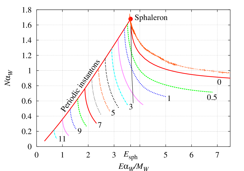
Figure 2: Lines of $F(E,N)=\mathrm{const}$. The lines are labeled by the values of the suppression exponent $-\alpha_{W}\log\sigma=4\pi F$. The line labeled by $0$ ($F=0$) is the boundary of the classically allowed region. The “fuzzy” line represents the approximate boundary of the classically allowed region found in the over-barrier calculations of Ref. Rebbi:1996zx .

The details of our numerical procedure are given elsewhere Bezrukov:2003er . Here we concentrate on our results. Clearly, only a part of $(E,N)$ plane is accessible to numerical study: the difficulty of the calculation increases at higher energies and smaller number of particles, as the solutions get sharper and linearize slower at large negative times. The region of $(E,N)$ plane covered in our study is shown in Fig. 2, where we present the results for $F(E,N)$. Before discussing the tunneling exponent $F(E,N)$, let us comment on various types of solutions we have found. The upper left line is the line of periodic instantons. These are solutions to the boundary value problem with $\theta=0$ Khlebnikov:1991th ; Bonini:1999fc , which correspond to transitions with the smallest tunneling exponent $F$ for given energy. The line of periodic instantons ends at the sphaleron point. The almost vertical line beginning at the sphaleron in Fig. 2 separates two parts of the classically forbidden region in which the solutions have qualitatively different properties. To the left of this line, the solutions are real on the Minkowskian part CD of the contour, and rapidly dissipate at large times forming spherical waves. This is illustrated in Fig. 3 where the field $\zeta=\beta-i\alpha$ is shown for a solution with relatively low energy. On the other hand, in the right part of the forbidden region, the solutions are complex on the part CD of the contour, and obey the reality condition (3b) only asymptotically. Part of the energy is emitted away in the form of spherical waves, but there remains a lump of energy near the origin, as illustrated in Fig. 4. We have checked that this remaining lump is nothing but the sphaleron.

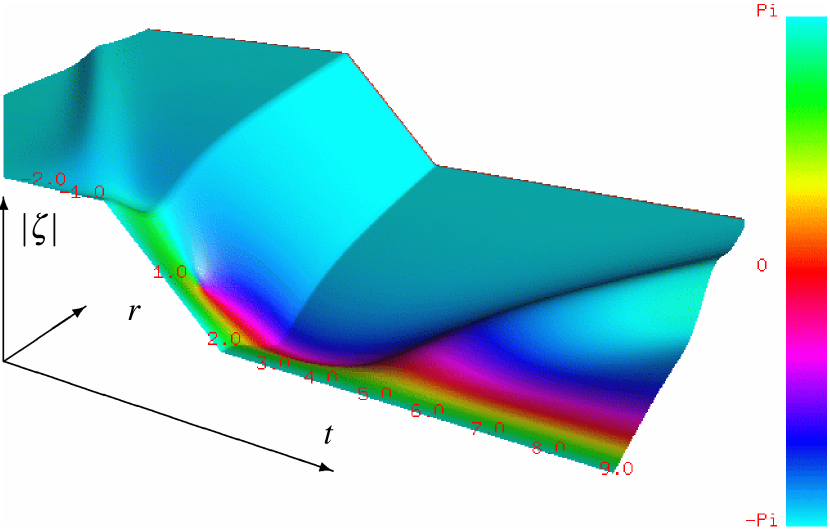
Figure 3: The field $\zeta$ for a solution with $N=1/\alpha_{W}$ and $E=3.35M_{W}/\alpha_{W}$. The color tracks the phase of the field, whose behavior indeed shows the correct topology. The part corresponding to the Euclidean evolution is inclined for visualization purposes.

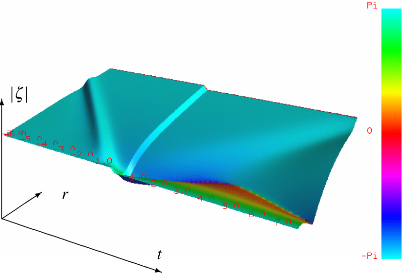
Figure 4: Field $\zeta$ for a solution with $N=1/\alpha_{W}$ and $E=4.48M_{W}/\alpha_{W}$.

The physical interpretation of the two types of solutions is as follows. At low energies, the system tunnels directly to the neighboring gauge theory vacuum plus linear excitations above it. At energies higher than the sphaleron energy (precisely, to the right of the almost vertical line in Fig. 2), the system ends up close to the sphaleron, with extra outgoing waves in the sphaleron background. In the latter case the system jumps on top of the barrier. This process is not precisely what is usually meant by tunneling; still it occurs with exponentially small probability which may be attributed to the rearrangement of the system from a collection of highly energetic incoming waves to the soft lump of the fields given by the sphaleron. The method of obtaining solutions of the second type was proposed in Ref. Bezrukov:2003yf , and we make use of this method in our work (see Ref. Bezrukov:2003er for details).

Let us now concentrate on the results for the tunneling exponent $F(E,N)$. Our data are in agreement with analytical results for $F(E,N)$ in the low energy region, see Ref. Bezrukov:2003zn for details. Another interesting comparison can be made with the results of Ref Rebbi:1996zx , where a Monte-Carlo technique was used to find real-time overbarrier solutions close to the boundary of the classically allowed region. This technique produced an approximation (and, at the same time, an upper bound) for the boundary of the classically allowed region. It is seen that the results of Ref. Rebbi:1996zx are reasonably close to the boundary of the classically allowed region found in our calculations.

To get insight into the suppression factor $F_{HG}(E)$ for actual particle collisions, we have to extrapolate our data to $N=0$, see Eq. (2). We present here two types of extrapolation. The first one produces lower bounds on the suppression exponent $F_{HG}(E)$ itself, while the second one gives an estimate for $F_{HG}(E)$. While the latter extrapolation has stronger predictive power at relatively low energies, $E\lesssim 2E_{\mathrm{sph}}$, the former extends to much higher energies, so the two are complementary.

We begin with the lower bounds on $F_{HG}(E)$. One way to obtain a lower bound is to make use of Eq. (6), together with the fact that $\theta$ increases as $N$ gets smaller. Hence, a lower bound on $F_{HG}(E)$ is obtained by simply continuing $F(E,N)$ with a linear function of $N$ for each energy. This bound is shown in Figs. 5, 6, dashed line. It indicates that up to the energy $8M_{W}/\alpha_{W}\simeq 20\mathrm{TeV}$ the suppression is still high: the suppression factor is smaller than $\mathrm{e}^{-60}\sim 10^{-26}$ for $\alpha_{W}\simeq 1/30$.

Figure 5: Lower bounds on the suppression exponent for two-particle collisions, dashed and dashed-dotted lines. The dotted line is the estimate of Refs. Ringwald:2002sw ; Ringwald:2003px .

Figure 6: Estimate of the suppression exponent for two-particle collisions $F_{HG}(E)$ (solid line), lower bound on $F_{HG}(E)$ (dashed line), low energy analytic prediction (8) (rare dotted line) and analytic estimate of Refs. Ringwald:2002sw ; Ringwald:2003px (dotted line).

Another lower bound, the best we can obtain at very high energies, is constructed by exploiting the observation that the lines of constant $F$ in $(E,N)$ plane have positive curvature (see Fig. 2). So, the lower bound is obtained by extrapolating these lines linearly to $N=0$. This bound is displayed in Fig. 5, dashed-dotted line. One can see that exponential suppression continues up to the energy of at least $250~{}\mathrm{TeV}$.

Let us now come to the second type of extrapolation which we make to estimate $F_{HG}(E)$ itself. We find it appropriate to use Eq. (5). The point is that the function $T(N)$ at fixed energy is approximately linear in $N$. This property has been shown analytically for low energies Bezrukov:2003zn , while for all energies it follows from our numerical data. [This is in contrast to the behavior of $F(E,N)$: the analytical results at low energy show that for fixed $E$, this function behaves as $N\log N$ as $N\to 0$ Bezrukov:2003zn .] We thus extrapolate $T(N,E$) linearly to $N=0$ along $E=\mathrm{const}$, and then integrate Eq. (5) at $N=0$ to obtain the suppression exponent $F_{HG}(E)$ for two-particle collisions. This estimate is shown in Fig. 6, solid line. It is instructive to compare it to the one loop analytic result Khoze:1991bm ; Arnold:1991cx ; Diakonov:LINPSchool1991 ; Mueller:1991fa , which gives three terms in the low-energy expansion,

$$\frac{4\pi}{\alpha_{W}}F(E)=\frac{4\pi}{\alpha_{W}}\left[1-\frac{9}{8}\left(\frac{E}{E_{0}}\right)^{4/3}+\frac{9}{16}\left(\frac{E}{E_{0}}\right)^{2}\right],$$ (8)

where $E_{0}=\sqrt{6}\pi M_{W}/\alpha_{W}$. We see that our numerical data are (somewhat unexpectedly) very close to the one loop result (8) up to the sphaleron energy. In this energy region, they are consistent also with the analytic estimate of Refs. Ringwald:2002sw ; Ringwald:2003px . On the other hand, the behavior of $F_{HG}(E)$ changes dramatically at $E\gtrsim E_{\mathrm{sph}}$. We attribute this to the change in the tunneling behavior—at $E\gtrsim E_{\mathrm{sph}}$ the system tunnels “on top of the barrier”. Our numerical data show that the suppression exponent $F_{HG}(E)$ flattens out, and topology changing processes are in fact much heavier suppressed at $E\gtrsim E_{\mathrm{sph}}$ as compared to the estimate (8) and the estimate of Refs. Ringwald:2002sw ; Ringwald:2003px .

Thus, our numerical results, albeit covering a limited range of energies and initial particle numbers, enable us to obtain both a lower bound for and an actual estimate of the suppression exponent for the topology changing two-particle cross-section in the electroweak theory well above the sphaleron energy. This cross section remains exponentially suppressed up to very high energies of at least $250~{}\mathrm{TeV}$. In fact, the energy, if any, at which the exponential suppression disappears, is most likely much higher, as suggested by comparison of our lower bound and actual estimate at energies exceeding significantly $E_{\mathrm{sph}}$, see Fig. 6.

- (1) F. R. Klinkhamer and N. S. Manton, Phys. Rev. D30, 2212 (1984).
- (2) G. ’t Hooft, Phys. Rev. D14, 3432 (1976).
- (3) A. Ringwald, Nucl. Phys. B330, 1 (1990).
- (4) O. Espinosa, Nucl. Phys. B343, 310 (1990).
- (5) L. McLerran, A. Vainshtein and M. Voloshin, Phys. Rev. D42, 171 (1990).
- (6) S. Y. Khlebnikov, V. A. Rubakov and P. G. Tinyakov, Nucl. Phys. B350, 441 (1991).
- (7) L. G. Yaffe, Scattering amplitudes in instanton backgrounds, in Santa Fe SSC Workshop, pp. 46–63, 1990.
- (8) P. B. Arnold and M. P. Mattis, Phys. Rev. D42, 1738 (1990).
- (9) M. P. Mattis, Phys. Rept. 214, 159 (1992).
- (10) P. G. Tinyakov, Int. J. Mod. Phys. A8, 1823 (1993).
- (11) V. A. Rubakov and M. E. Shaposhnikov, Usp. Fiz. Nauk 166, 493 (1996), [hep-ph/9603208].
- (12) A. Ringwald, Phys. Lett. B555, 227 (2003), [hep-ph/0212099].
- (13) A. Ringwald, hep-ph/0302112.
- (14) C. Rebbi and J. Singleton, Robert, Phys. Rev. D54, 1020 (1996), [hep-ph/9601260].
- (15) O. R. Espinosa, Nucl. Phys. B375, 263 (1992).
- (16) V. A. Rubakov and P. G. Tinyakov, Phys. Lett. B279, 165 (1992).
- (17) P. G. Tinyakov, Phys. Lett. B284, 410 (1992).
- (18) V. A. Rubakov, D. T. Son and P. G. Tinyakov, Phys. Lett. B287, 342 (1992).
- (19) A. H. Mueller, Nucl. Phys. B401, 93 (1993).
- (20) G. F. Bonini, A. G. Cohen, C. Rebbi and V. A. Rubakov, quant-ph/9901062.
- (21) G. F. Bonini, A. G. Cohen, C. Rebbi and V. A. Rubakov, Phys. Rev. D60, 076004 (1999), [hep-ph/9901226].
- (22) F. Bezrukov and D. Levkov, quant-ph/0301022.
- (23) A. N. Kuznetsov and P. G. Tinyakov, Phys. Rev. D56, 1156 (1997), [hep-ph/9703256].
- (24) F. Bezrukov, C. Rebbi, V. Rubakov and P. Tinyakov, hep-ph/0110109.
- (25) B. Ratra and L. G. Yaffe, Phys. Lett. B205, 57 (1988).
- (26) F. Bezrukov, D. Levkov, C. Rebbi, V. Rubakov and P. Tinyakov, hep-ph/0304180.
- (27) S. Y. Khlebnikov, V. A. Rubakov and P. G. Tinyakov, Nucl. Phys. B367, 334 (1991).
- (28) G. F. Bonini et al., Periodic instantons in SU(2) Yang-Mills-Higgs theory, in Copenhagen 1998, Strong and electroweak matter, pp. 173–182, 1999, [hep-ph/9905243].
- (29) F. Bezrukov and D. Levkov, hep-th/0303136.
- (30) V. V. Khoze and A. Ringwald, Nucl. Phys. B355, 351 (1991).
- (31) P. B. Arnold and M. P. Mattis, Mod. Phys. Lett. A6, 2059 (1991).
- (32) D. I. Diakonov and V. Y. Petrov, in Proc. XXVI LINP Winter School. LINP, Leningrad, 1991.
- (33) A. H. Mueller, Nucl. Phys. B364, 109 (1991).