Abstract

We note that the phenomenon of perturbative saturation leads to transverse momentum broadening in the spectrum of partons produced in hadronic collisions. This broadening has a simple interpretation as parton level Cronin effect for systems in which saturation is generated by the ”tree level” Glauber-Mueller mechanism. For systems where the broadening results form the nonlinear QCD evolution to high energy, the presence or absence of Cronin effect depends crucially on the quantitative behavior of the gluon distribution functions at transverse momenta $k_{t}$ outside the so called scaling window. We discuss the relation of this phenomenon to the recent analysis by Kharzeev-Levin-McLerran of the momentum and centrality dependence of particle production in nucleus-nucleus collisions at RHIC.

1 Introduction

The phenomenon of perturbative saturation has been the focus of intensive study in recent years. Since the appearance of the first RHIC data, saturation based ideas have motivated several attempts at understanding bulk properties of ultra-relativistic heavy ion collisions such as the multiplicity, rapidity distribution and centrality dependence of particle production [1, 2]. In particular the recent work [2] suggests that the saturating properties of the nuclear gluon distribution may be responsible for the $N_{\rm part}$ scaling of charged particle multiplicity at $2<p_{t}<8$ GeV with centrality in RHIC data. It is undoubtedly true that saturation effects suppress the number of gluons below the saturation momentum $Q_{s}$ in the nuclear wave function. It is then very plausible that the number of produced particles at $p_{t}<Q_{s}$ is also suppressed relative to simple perturbative prediction. The value of $Q_{s}^{2}$ is estimated to be of order $2$ GeV² for most central collisions at RHIC [1]. The suggestion of [2] goes beyond this simple statement and implies that the suppression persists also at higher momenta, namely in the so called scaling window $Q_{s}<p_{t}<Q_{s}^{2}/Q_{0}$.

On the other hand one expects a competing effect of transverse momentum broadening due to multiple rescatterings in the final state, the so called Cronin effect. This should enhance the number of particles produced in the intermediate momentum range and thus works against the saturation argument. The purpose of this note is to show that there is no outright contradiction between the appearance of the Cronin effect and the expectations based on the saturation scenario and that, in fact, the Cronin enhancement is inherent in some realizations of saturation physics. We show here that saturation models based on multiple rescattering lead to the relation

$${dN^{\rm sat}\over d^{2}p_{t}}>{dN^{\rm pert}\over d^{2}p_{t}}$$ (1)

for all $p_{t}>Q_{s}$. This relation leads to Cronin enhancement when comparing gluon production in central and peripheral collisions.

For saturation models based not on multiple rescattering but rather on coherent suppression at low $x$ the situation is more complicated. Here it is also true that the number of gluons produced in the intermediate momentum range is greater than the prediction of the leading order perturbation theory. This overall enhancement is the result of the increase of the number of gluons in the nuclear wave function due to low $x$ evolution. The transverse momentum broadening is also present. This is manifested by the anomalous dimension generated by the low $x$ evolution, so that the decrease of the evolved distribution with momentum is very slow. However, whether this broadening results in the Cronin enhancement is determined by the behavior of saturated gluon distribution at high transverse momenta. The momenta which are important are those above the scaling window inside which the value of the anomalous dimension is analytically understood. If the distribution above the scaling window approaches quickly the leading order perturbative one, the Cronin effect is indeed generated. However if the distribution continues to vary much slower than $1/p_{t}^{2}$, the (properly normalized) multiplicity of produced gluons is always smaller for central collisions than for the peripheral ones.

In this light, the results of  [2] should be understood in the following way. In a particular saturation ansatz considered in  [2] for $p_{t}$ in the scaling window, ${dN^{\rm sat}\over d^{2}p_{t}}$ as a function of centrality is indeed proportional to the number of participants $N_{\rm part}$. However its value is always greater than that for the leading order perturbative prediction for the same momentum, even though the latter is proportional to the number of collisions $N_{\rm coll}\propto N^{4/3}_{\rm part}$. This holds as long as the transverse momentum in question is greater than the saturation momentum for the most central collisions considered. Thus according to the saturation scenario, the number of produced particles in the intermediate transverse momentum range is enhanced and not suppressed relative to the leading order perturbative one. This enhancement in the overall production may or may not result in the Cronin enhancement when comparing the production rates for central versus peripheral collisions, as the evolution is equally effective for all impact parameters.

Before we proceed further, we wish to make clear the following points. First, to calculate the gluon production we use the $k_{t}$ factorized formalism as in [1, 2]. Although it has not been proved to hold for this process and is likely not to be strictly valid, one may hope as in  [1] that it gives a qualitatively reasonable description of gluon production. Second, in this note we only address the multiplicity of produced gluons. For comparison with experimental data, this quantity has to be convoluted with gluon fragmentation functions to convert it to the number of produced hadrons. This introduces additional uncertainties related to our limited knowledge of the dynamics of the system between the time of production and the time of hadronization [3], and the possible medium-dependence of parton fragmentation  [4]. Thus our results have to be paralleled to those of  [2] prior to convolution with fragmentation functions.

The simple $k_{t}$-factorized formula for the gluon yield at central rapidity in a collision of identical nuclei  [7] used in  [2] is

$$E{d\sigma\over d^{3}p\,d^{2}b}={4\pi^{2}\alpha_{s}S_{AA}(b)N_{c}\over N_{c}^{2}-1}{1\over p_{t}^{2}}\int d^{2}k_{t}\,\phi_{A}(y,k_{t})\,\phi_{A}(y,p_{t}-k_{t})\,.$$ (2)

Here $S_{AA}(b)$ is the overlap area in the transverse plane between the nuclei at fixed impact parameter $b$, $y$ is the rapidity difference between the central rapidity and the fragmentation region and $\phi_{A}(y,k_{t})$ is the intrinsic momentum dependent nuclear gluon distribution function, related to the standard gluon distribution by

$$\phi_{A}(y,k_{t})={d(xG_{A}(x,k^{2}_{t}))\over d^{2}k_{t}\,d^{2}b}\,.$$ (3)

Eq. (2) itself is an approximation even within the $k_{t}$-factorization scheme for two reasons. First, the gluon distribution is considered to be effectively impact parameter independent and taken at some representative impact parameter inside the overlap region. Second the rapidity of both distribution functions is taken to be the same rather than integrating over the relative rapidity of the two distributions. This amounts to the assumption that the gluons are produced locally in rapidity and keep the same rapidity label as in the parent distribution function. The first assumption in principle is easily relaxed by considering $b$-dependent distributions, although it makes the calculation considerably more cumbersome. The second assumption is more questionable. One certainly expects ”migration” in rapidity during the interaction, and in particular the relevant rapidities should depend on the produced transverse momentum. This is certainly the case in the collinear factorized perturbative formalism, where the parent rapidities are taken at $x=k_{t}/\sqrt{s}$. However in the present case the production is not necessarily through the $2\rightarrow 2$ process, and thus the rapidities are not fixed in the same way. Keeping these caveats in mind, we now consider the implications of Eq. (2).

In a purely perturbative approach, neglecting the effects of saturation the gluon distribution function at impact parameter $b$ has the shape

$$\phi_{A}^{\rm pert}(k_{t},b)={\alpha_{s}(N_{c}^{2}-1)\over 2\pi^{2}}K{\rho_{\rm part}(b)\over 2}{1\over(k_{t}+\Lambda_{QCD})^{2}}\,,$$ (4)

where $\rho_{\rm part}(b)$ is the density of participants, taken as reference for $A-A$ collisions. The role of $\Lambda_{QCD}$ in the denominator is to regulate the gluon distribution in the infrared. The additional numerical multiplicative factor $K$ reflects the fact that the gluons at low $x$ originate not only from the valence quarks, but also from the sea quarks and energetic gluons.

2 Models for the gluon distribution

Saturation effects modify the gluon distribution so that it is suppressed at low momenta $|k_{t}|<Q_{s}$. There are several models in the literature which provide such saturated distribution function. In this note we consider two types of models.

2.1 McLerran–Venugopalan gluon  [8]

The McLerran-Venugopalan model [8] achieves saturation by taking into account the Glauber-Mueller multiple scattering effects. The intrinsic glue distribution in this model was calculated in  [9, 10]

$$\phi^{\rm MV}_{A}(k_{t})={N^{2}_{c}-1\over 4\pi^{4}\alpha_{s}N_{c}}\int{d^{2}{\bf x}\over{\bf x}^{2}}\left(1-e^{-{\bf x}^{2}Q_{s}^{2}({\bf x}^{2})/4}\right)\,e^{i\,k_{t}\cdot{\bf x}}\,.$$ (5)

We will take the saturation momentum to be ${\bf x}$-dependent following  [1]

$$Q_{s}^{2}({\bf x}^{2},b)={4\pi^{2}\alpha_{s}N_{c}\over N_{c}^{2}-1}\,xG(x,1/{\bf x}^{2}){\rho_{\rm part}(b)\over 2}\,,$$ (6)

with $G(x,k_{t}^{2}=1/{\bf x}^{2})$ being the nucleon gluon distribution. We will take the gluon distribution in the nucleon to be of the simple perturbative form  [11]

$$xG(x,1/{\bf x}^{2})=K\ \frac{\alpha_{s}(N_{c}^{2}-1)}{2\pi}\ln\left(\frac{1}{{\bf x}^{2}\Lambda^{2}_{\rm QCD}}+a\right)\,.$$ (7)

The small regulator $a=\frac{1}{{\bf x}_{c}^{2}\Lambda^{2}_{\rm QCD}}$ ensures that the saturation momentum stays positive for ${\bf x}^{2}\gg{\bf x}_{c}^{2}$. For the numerical evaluations we choose $x_{c}=3~{}{\rm GeV}^{-1}$, such that for momenta $k_{t}\geq O(1~{}{\rm GeV})$ the sensitivity on the infrared cut off $a$ is negligible. We take $\Lambda_{\rm QCD}=0.2~{}{\rm GeV}$, and $\alpha_{s}=0.5$. The saturation scale $Q_{s}^{2}(b)$ is obtained from the solution of the implicit equation Eq. (6), when evaluated at ${\bf x}^{2}=1/Q_{s}^{2}(b)$. At $b=0$ we fix $Q_{s}^{2}=2~{}{\rm GeV}^{2}$ throughout this paper; this corresponds to $K=1.8$ in Eq. (7).

The MV distribution appears in the light cone gauge calculation as the average of the gluon number density operator in the state with random distribution of color charges distributed with the nuclear density  [10]. On the other hand as shown in  [9], in the covariant gauge calculation of DIS-like processes it accounts precisely for the rescattering of the produced gluon inside the nucleus. The effect of these multiple rescatterings is to broaden the gluon transverse momentum spectrum by the amount $\Delta k^{2}_{t}\sim Q_{s}^{2}$. Accordingly, the low momentum part of $\phi^{\rm MV}_{A}$ is suppressed relative to the perturbative gluon, the region around $k_{t}\sim Q_{s}$ is enhanced, while at large momenta $k_{t}\gg Q_{s}$ there is no appreciable change relative to the perturbative gluon. Fig.1a shows the ratio of the MV gluon to the perturbative one as a function of momentum for fixed coupling constant $\alpha_{s}=0.5$. The multiple rescatterings do not change the total number of gluons but only redistribute the gluon momentum. Thus the gluon distribution $G(Q^{2})$ calculated with $\phi_{A}^{\rm MV}$ is the same as the perturbative one for $Q^{2}\gg Q_{s}^{2}$.

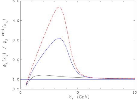
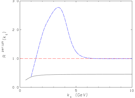
Figure 1: a). The unintegrated gluon distribution function, normalized to the corresponding perturbative one, as function of $k_{t}$ for fixed $\rho_{\rm part}=3.1~{}{\rm fm^{-2}}$ and for $Q_{s}^{2}\simeq 2~{}{\rm GeV}^{2}$; solid curve: gluon distribution in the McLerran-Venugopalan model  [8], dot-dashed curve: model (10) - (12) for the evolved gluon distribution. The dashed curve is for the anomalous dimension $\gamma=0.5$. b). The ratio $R^{\rm periph}$ in Eq. (17) for the gluon distributions Eq. (10) (dot-dashed curve) and Eq. (13) (solid curve).

In a DIS-like process with a probe directly coupled to gluons, the intrinsic momentum distribution would be directly proportional to the spectrum of final state gluons. The Cronin effect is therefore present in the MV gluon ab initio. This has been noticed in  [12]. The question we are interested in, is to what extent this effect shows up in nuclear collisions.

2.2 Evolved gluons

The MV gluon distribution does not contain any evolution in $x$. One way to introduce the $x$ dependence is to adopt the Golec-Biernat-Wüsthoff procedure  [13], whereby the saturation momentum is taken to be energy dependent with the factor $x^{-\lambda}$, with $\lambda=0.2-0.3$. In this paper we are not going to explore the energy dependence of the spectrum, and thus for our purposes the energy independent MV ansatz is sufficient.

Another type of saturated gluon distribution has been used in  [2]. The energy dependence in the RHIC energy range is not large enough to allow one to explore the perturbatively predicted $x$ dependence of the distribution function. One can nevertheless consider $\phi$ (at both 130 and 200 GeV) as being evolved by the perturbative evolution from lower energies. Such an energy evolution leaves a distinctive imprint on the $k_{t}$ dependence of the gluon. Although the solution of the nonlinear QCD evolution equation  [14] has not been analyzed in great detail, its qualitative features have been discussed in  [15]. It has been argued in  [15] that in the wide region of momenta $Q_{s}(x)<|k_{t}|<{Q_{s}^{2}(x)\over Q_{0}}$ the evolved distribution behaves as

$$\phi^{\rm NLE}_{A}(k_{t})\propto\left[{Q_{s}^{2}\over k_{t}^{2}}\right]^{\gamma}$$ (8)

with the anomalous dimension

$$\gamma=0.64\,.$$ (9)

A slightly different analysis of  [2] based on doubly logarithmic approximation suggests $\gamma=0.5$. In either case due to the large anomalous dimension, $\phi_{A}^{\rm NLE}$ is very significantly enhanced over the perturbative $\phi_{A}^{\rm pert}$ in the wide range of momenta. At asymptotically large momenta $\phi_{A}^{\rm NLE}$ again reduces to the perturbative expression.

As we will see in the following it is important to know how the distribution behaves outside the scaling window. The behavior outside the scaling window is not known analytically. One expects that at asymptotically large momenta the behavior of $\phi_{A}^{\rm NLE}$ is perturbative, and therefore $\gamma_{|k_{t}|\rightarrow\infty}\rightarrow 1$. The crossover from the scaling with the anomalous dimension to the perturbative one can in principle be either sharp at the edge of the window, or can be very gradual and slow. To explore the possible differences between the fast and slow crossovers we will use two parametrizations of the distribution function.

To model the function with the fast crossover we take for illustration

$$\phi^{\rm NLEF}_{A}(k_{t})={N^{2}_{c}-1\over 4\pi^{3}\alpha_{s}N_{c}}\left({\frac{{\hat{Q}}^{2}_{s}}{k_{t}^{2}+{\hat{Q}}_{s}^{2}}}\right)^{\gamma(k_{t})}\,,$$ (10)

where

$${\hat{Q}}_{s}^{2}={\hat{Q}}_{s}^{2}(b)=K~{}{2\pi\alpha_{s}^{2}N_{c}}\,{\rho_{\rm part}(b)\over 2}\,,$$ (11)

and

$$\gamma(k_{t})=\frac{1+0.64\,w(k_{t})}{1+w(k_{t})}\,,\qquad w(k_{t})=\left(\,\frac{10\,Q_{s}^{2}(b)}{(k_{t}+~{}\Lambda_{\rm QCD})^{2}}\right)^{6}\,.$$ (12)

Here, $Q_{s}^{2}(b)=4\,{\hat{Q}}_{s}^{2}(b)$, consistent with Eq.  (6) at $\rho_{\rm part}=3.1\,\hbox{fm}^{-2}$.

The parametrization of $\phi^{\rm NLE}_{A}(k_{t})$ is chosen to be consistent with the required behavior at large $k_{t}$ as well as at $k_{t}=O(Q_{s})$  [15]. The width of the scaling window in our parametrization is $\sim 3\,Q_{s}$. For $k_{t}<Q_{s}$, the gluon $\phi_{A}^{\rm NLE}$ is supposed to saturate or grow at most logarithmically. In our ansatz this saturation is ensured by the presence of the term $\hat{Q}^{2}_{s}$ in the denominator of Eq. (10).

To model the possibility of the slow crossover we will take simply the function with fixed anomalous dimension:

$$\phi^{\rm NLES}_{A}(k_{t})={N^{2}_{c}-1\over 4\pi^{3}\alpha_{s}N_{c}}\left({\frac{{\hat{Q}}^{2}_{s}}{k_{t}^{2}+{\hat{Q}}_{s}^{2}}}\right)^{0.64}\,,$$ (13)

Although this function never approaches the perturbative asymptotics, for the purposes of numerical evaluation it is indistinguishable from a function with slowly varying $\gamma(k)$.

We note that Eq. (10) parametrizes the gluon distribution directly in momentum space. We found that this is the simplest way to generate an acceptable $\phi$ to be used in the framework of Eq. (2). Alternatively one could try to define $\phi$ via the frequently used relation involving the dipole scattering cross section $N({\bf x})$  [15]:

$$\phi^{\rm NLE}_{A}(k_{t})={N^{2}_{c}-1\over 4\pi^{4}\alpha_{s}N_{c}}\int{d^{2}{\bf x}\over{\bf x}^{2}}N({\bf x})e^{i\,k_{t}{\bf x}}\,.$$ (14)

where

$$N({\bf x})=\frac{\left({\bf x}^{2}Q_{s}^{2}({\bf x}^{2})/4\right)^{\gamma}}{1+\left({\bf x}^{2}Q_{s}^{2}({\bf x}^{2})/4\right)^{\gamma}}\,,$$ (15)

with $\gamma(x)$ approaching $\gamma=0.64$ at small values of $1/Q_{s}>x>\Lambda_{\rm QCD}/Q_{s}^{2}$ in a way similar to Eq. (12). Although strictly speaking $\phi_{A}(k_{t})$ is defined by the relation Eq. (14) only at large $k_{t}$, naively one could expect it to be also reasonable at $k_{t}\sim Q_{s}$. However it turns out not always to be the case. The Fourier transform in Eq. (14) is not only sensitive to $x\sim 1/k_{t}$ but to all $x<1/k_{t}$. As a result depending on details of the parametrization of $\gamma(x)$, we sometimes found ”oscillating” unintegrated gluon functions which for some momenta were even negative. In general, this indicates that one should be very careful using relation Eq. (14), as even for a reasonable $N(x)$ it can produce unacceptable $\phi_{A}^{\rm NLE}(k_{t})$.

As seen from Fig.1, the qualitative features of the gluon distribution in the MV model (5) and the scaling models (10) are to some extent similar. When compared to the leading order perturbative distribution Eq. (4) they show suppression at $k_{t}\ll Q_{s}$ and enhancement at $k_{t}>Q_{s}$. In Fig.1a, we show the ratio

$$R^{\rm pert}=\phi_{A}(k_{t})/\phi^{\rm pert}_{A}(k_{t})\,.$$ (16)

In the scaling model the enhancement is much more pronounced. It is clear that using the same ansatz, but with $\gamma=0.5$ rather than $\gamma=0.64$ would make this enhancement even greater.

In relation to the MV gluon the perturbative distribution Eq. (4) is the relevant distribution to be used to model the peripheral collisions. For the evolved functions a more meaningful comparison is with the “peripheral” distribution of the same functional form as $\phi_{A}^{\rm NLE}$ but with a smaller value of $Q_{s}$. In Fig.1b we plot the ratios

$$R_{\rm NLEF(S)}^{\rm periph}=\frac{\phi_{A}^{\rm NLEF(S)}(b=0,k_{t})/\rho_{\rm part}(b=0)}{\phi_{A}^{\rm NLEF(S)}(b=13\,{\rm fm},k_{t})/\rho_{\rm part}(b=13\,{\rm fm})}$$ (17)

with $Q_{s}$ corresponding to $\rho_{\rm part}=3.1\,{\rm fm}^{-2}$ and $\rho_{\rm part}=0.35\,{\rm fm}^{-2}$, (the values of impact parameters $b=0$ and $b=13\,{\rm fm}$) respectively. We observe that the ratios for $\phi^{\rm NLEF}_{A}$ and $\phi^{\rm NLES}_{A}$ are very different. While the ratio $R^{\rm periph}_{\rm NLEF}$ exhibits enhancement for the momenta in the scaling window, no such enhancement is seen in $R^{\rm periph}_{\rm NLES}$. The reason is that with the ansatz $\phi_{A}^{\rm NLEF}$ as long as $k_{t}$ is outside the scaling window of the peripheral distribution, but inside the window of the central one (that is for $3\,Q_{s}(b=13{\rm fm})<k_{t}<3Q_{s}(b=0)$) the ratio $R_{\rm NLEF}^{\rm periph}$ is practically equal to $R^{\rm pert}$. This is not the case for $\phi_{A}^{\rm NLES}$ because of a very slow approach to asymptotic behavior. Instead, for all momenta of interest

$$R^{\rm periph}_{\rm NLES}=\left({Q_{s}^{2}(b=0)\over Q_{s}^{2}(b=13\,{\rm fm})}\right)^{\gamma-1}={\rho_{\rm part}(b=13\,{\rm fm})\over\rho(b=0)}^{1-\gamma}<1\ .$$ (18)

We note that the physics of the enhancement of $R^{\rm pert}$ for $\phi_{A}^{\rm NLE}$ is different from that of $\phi_{A}^{\rm MV}$. According to  [15] and  [2] the anomalous dimension of the evolved distribution is a direct consequence of the linear BFKL (or doubly logarithmic) evolution and is not significantly affected by the nonlinearity of BK equation. As opposed to multiple rescatterings resummed in $\phi_{A}^{\rm MV}$, the BFKL evolution greatly increases the total number of gluons relative to the perturbative distribution. Thus the enhancement of $\phi_{A}^{\rm NLE}$ is not due to the gluon number conserving redistribution of the gluon momentum, but rather due to the BFKL growth of the total number of gluons. The slow fall off of $\phi_{A}^{\rm NLE}$ with momentum in the scaling window and the associated clear momentum broadening is the result of the BFKL diffusion, which fills the phase space very far from the momentum at which the distribution is peaked at initial energy.

Although some qualitative features of saturating gluon distributions appear to be model-independent, quantitative results can vary significantly, see Fig.1a and Fig.1b. In the rest of this paper, we discuss the implications of this model-dependence for the spectrum Eq. (2), and we study the behavior of $dN/d^{2}p_{t}$ as a function of transverse momentum and centrality.

3 Gluon production in A-A collisions

For the perturbative gluon distribution Eq. (4), the main contribution to the integral in Eq. (2) comes from the region of phase space $k_{t}-p_{t}\sim 0$ and $k_{t}\sim 0,\ \ \ p_{t}-k_{t}\sim p_{t}$. The contribution from the bulk of the phase space $k_{t}\sim k_{t}-p_{t}\sim p_{t}$ is logarithmically suppressed due to the fast decrease of the perturbative distribution function with $k_{t}$. One finds

$$\frac{dN^{\rm pert}(b)}{dy\,d^{2}p_{t}}\Bigg{|}_{y=0}=2S_{AA}(b){N_{c}^{2}-1\over 4\pi^{3}\alpha_{s}N_{c}}{{\hat{Q}}_{s}^{4}(b)\over p^{4}_{t}}~{}\left(\ln{p_{t}^{2}\over 4\Lambda^{2}_{\rm QCD}}+2\gamma_{E}\right)\,,$$ (19)

where $\gamma_{E}$ is the Euler constant. With Eq. (11) this spectrum scales with $N_{\rm coll}\propto S_{AA}(b)\,\rho_{\rm part}^{2}(b)$ as expected perturbatively.

For the saturated gluon distribution in the MV model the gluon yield Eq. (2) is expressed by

$$\frac{dN(b)}{dy\,d^{2}p_{t}}\Bigg{|}_{y=0}=\frac{2}{\pi^{3}}\,\frac{N_{c}^{2}-1}{\alpha_{s}\,N_{c}}\,\frac{S_{AA}(b)}{p_{t}^{2}}\,\int_{0}^{\infty}\frac{dx}{x^{3}}\,\left(1-e^{-{\bf x}^{2}Q_{s}^{2}({\bf x}^{2})/4}\right)^{2}\,\,J_{0}(p_{t}\,x)\,.$$ (20)

Since small momenta $p_{t}$ are suppressed in the MV gluon distribution, expression (20) is smaller than the perturbative one. For small $|p_{t}|$, the ${\bf x}$-dependence of the saturation scale Eq. (6) is frozen, and one finds

$$\frac{dN(b)}{dy\,d^{2}p_{t}}\Bigg{|}_{y=0}^{p_{t}\ll Q_{s}(b)}=\frac{1}{4\pi^{3}}\,\frac{N_{c}^{2}-1}{\alpha_{s}\,N_{c}}\,\frac{Q_{s}^{2}(b)\,S_{AA}(b)}{p_{t}^{2}}\,\ln(4)\,.$$ (21)

Thus, for small transverse momentum, the spectrum (21) scales with the number of participants, i.e.

$$N_{\rm part}(b)=S_{AA}(b)~{}\rho_{\rm part}(b)\,.$$ (22)

Numerically, however, we find that the limit (21) provides a fair approximation for the full expression (20) in a very small $\rho_{\rm part}(b)$-dependent region below $p_{t}<0.1$ GeV only.

In Fig.2 we plot the result of the numerical evaluation of the formula Eq. (20) normalized to the peripheral (perturbative) yield Eq. (19), i.e.

$$\frac{dN(b)}{dyd^{2}p_{t}}\Bigg{/}\frac{dN^{\rm pert}(b)}{dyd^{2}p_{t}}\,,$$ (23)

for $\rho_{\rm part}=3.1~{}({\rm fm^{-2}})$, and with $~{}Q_{s}^{2}=2~{}{\rm GeV^{2}}$. This corresponds to the normalized ratio of central over peripheral yields

$$\frac{1}{N_{\rm coll}(b=0)}\frac{dN(b=0)}{dyd^{2}p_{t}}\Bigg{/}\frac{1}{N_{\rm coll}(b=13\,\hbox{fm})}\frac{dN(b=13\,\hbox{fm})}{dyd^{2}p_{t}}\,.$$ (24)

To understand the $p_{t}$-dependence of (23) qualitatively, we consider the integral $\int d^{2}k_{t}$ $\phi_{A}(y,k_{t})$ $\phi_{A}(y,p_{t}-k_{t})$ in (2). For a saturated gluon distribution and $|p_{t}|>Q_{s}$, one does not gain a logarithmic enhancement factor from the low momentum region, $|k_{t}|\ll|p_{t}|$. However due to enhancement in the intermediate region one gets a bigger contribution to the integral from $|k_{t}|\sim|k_{t}-p_{t}|\sim Q_{s}$. Since both factors of $\phi$ are enhanced in this region, we expect that for some momentum range this enhancement will overcome the suppression in the small momentum range, and therefore will lead to a net excess of produced gluons relative to the perturbative result. This is seen in Fig.2 as a small but clear Cronin enhancement of the produced gluon number for momenta just above the saturation scale. The amount of enhancement depends on the value of the coupling constant, but qualitatively the phenomenon persists for any $\alpha_{s}$.

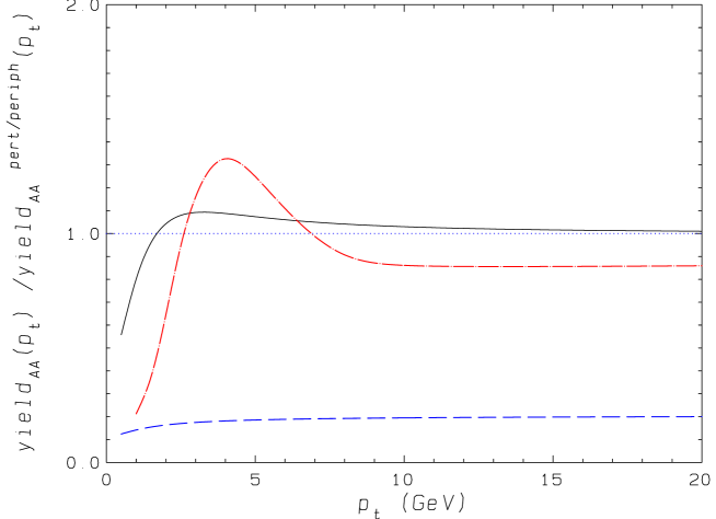
Figure 2: Cronin effect in the $p_{t}$-dependence of gluon production yields for head-on A-A collisions. Solid curve for the MV-gluon distribution normalized to the perturbative yield. The dot-dashed curve is for the evolved gluon distribution (10), the dashed one for the evolved gluon distribution (13), both normalized as in Eq.  (24).

For the evolved distributions $\phi_{A}^{\rm NLE}$, since the $k_{t}$ dependence is very slow, the contribution to the integral comes from a very large range of momenta - for $p_{t}$ in the scaling region the integral is dominated by $|k_{t}|\sim|k_{t}-p_{t}|\sim|p_{t}|$. This leads to a significant enhancement of gluon production for all $|p_{t}|>Q_{s}$ relative to the perturbative expression. It is however more interesting to consider the ratio of the central to peripheral yields. Again, taking $\rho_{\rm part}(b=0)=3.1\,{\rm fm}^{-2}$ and $\rho_{\rm part}(b=13)=0.35\,{\rm fm}^{-2}$ we display the results of the numerical integration of Eq. (2) in Fig.2. This plot mirrors the plot for a single distribution Fig.1b. The distribution $\phi^{\rm NLEF}_{A}$ displays a clear Cronin effect similar to the MV gluon, while $\phi_{A}^{\rm NLES}$ shows uniform suppression for the central/peripheral ratio for all momenta. Although the ratio of the yields for $\phi_{A}^{\rm NLEF}$ is smaller than unity at $p_{t}\sim 10-20{\rm GeV}$, we have checked numerically that at very large $p_{t}$ it slowly approaches unity from below. We thus conclude that the properties of the ratio are very sensitive to the way in which the distribution behaves outside the scaling window.

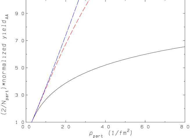
Figure 3: Centrality dependence of gluon production yields (2) in A-A collisions as a function of $\rho_{\rm part}~{}({\rm fm^{-2}})$, normalized to the yield in peripheral collisions, Eq. (25). Curves are calculated for the MV gluon distribution (5) and different values of $p_{t}$: solid curve: $p_{t}=0.25~{}{\rm GeV}$, dashed curve: $p_{t}=1.0~{}{\rm GeV}$, dot-dashed curve: $p_{t}=3.0~{}{\rm GeV}$.

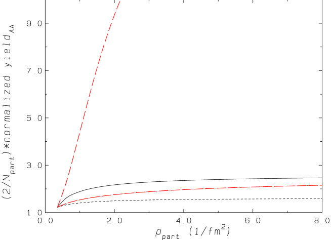
Figure 4: Centrality dependence as in Fig. 3, but with the gluons of Eq. (10) and Eq.  (13) for $p_{t}=$ 1 and 3 GeV. The solid and dashed lines correspond to Eq. (10) for $p_{t}=1$ GeV and $p_{t}=3$ GeV, respectively. The short-dashed ($p_{t}=$ 1 GeV) and dot-dashed ($p_{t}=3$ GeV) lines are calculated for the gluon distribution (13).

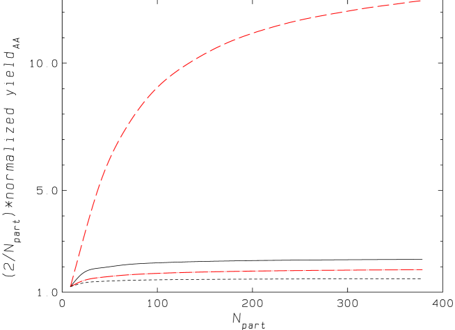
Figure 5: Normalized yield for evolved gluon distributions as a function of $N_{\rm part}$. Legend the same as on Fig.4. The largest value $N_{\rm part}=380$ corresponds to $\rho_{\rm part}=3.1~{}{\rm fm}^{-2}$ on Fig.4.

We discuss now to what extent the gluon spectrum (2) shows an approximate $N_{\rm part}$ or $N_{\rm coll}$ scaling in some kinematic regime. To this end, we plot the gluon yield normalized to the yield for peripheral collisions at $b=13.0~{}{\rm fm}$, corresponding to $\rho_{\rm part}=0.35~{}{\rm fm^{-2}}$  [1],

$$\frac{2}{N_{\rm part}(b)}~{}\frac{dN(b)}{dyd^{2}p_{t}}\Bigg{/}\frac{dN(b=13.0)}{dyd^{2}p_{t}}\,.$$ (25)

This quantity is plotted for the MV gluon in Fig.3 and for the evolved gluon distributions (10) and (13) in Fig.4, for various fixed values of $p_{t}$ as a function of $\rho_{\rm part}$. We also replot in Fig.5 this quantity for the evolved gluon as a function of $N_{\rm part}$ using the relation between $\rho_{\rm part}$ and $N_{\rm part}$ given in  [1]. We explore the dependence on $\rho_{\rm part}$ beyond the experimentally accessible range to illustrate better the functional dependence. For the MV gluon a steep increase with $\rho_{\rm part}$ indicative of $N_{\rm coll}$ scaling is found for $p_{t}\geq 1~{}{\rm GeV}$. For smaller transverse momentum, e.g. $p_{t}=0.25~{}{\rm GeV}$, the $\rho_{\rm part}$-dependence is seen to level off.

For the evolved gluon the centrality dependence is again sensitive to the large momentum behavior. For $\phi_{A}^{\rm NLEF}$ at $p_{t}=3\,{\rm GeV}$ the centrality dependence is similar to the MV gluon. One does not recover $N_{\rm part}$ scaling even in the enlarged centrality region $\rho_{\rm part}<8~{}{\rm fm^{-2}}$. The qualitative features of Figs.4 and 5 at small and large $\rho_{\rm part}$ at $p_{t}=3~{}{\rm GeV}$ can be understood as follows: At small $\rho_{\rm part}$, the saturation momentum $Q_{s}$ is small so that the scaling window does not exist; the overall yield scales with $N_{\rm coll}$, like the perturbative one. This $N_{\rm coll}$ behavior should persist as long as 3 GeV is above the scaling window, $3\,\hbox{GeV}>Q_{s}^{2}(b)/Q_{0}$ (for our parametrization $Q_{0}=0.5\,{\rm GeV}$). This is indeed seen for small $\rho_{\rm part}$ in Figs.4 and 5. In the other extreme, when $Q_{s}^{2}$ becomes very large and 3 GeV lies well inside the scaling window, the main contribution to the yield comes from the integration over the momentum in the scaling window and one obtains

$$\frac{dN(b)}{dyd^{2}p_{t}}\propto S(b)Q_{s}^{2\gamma}\,.$$ (26)

This dependence is much flatter. For $\gamma=0.5$ as in  [2], it scales with $N_{\rm part}$ rather than $N_{\rm coll}$. For the value $\gamma=0.64$ used here, the dependence is only slightly steeper. This is the argument given in  [2]. However, as we have shown above, at these large values of $Q_{s}$ the absolute magnitude of $\frac{dN(b)}{dyd^{2}p_{t}}$ is greater than that of $\frac{dN^{\rm pert}(b)}{dyd^{2}p_{t}}$. Hence there must be an intermediate region of $\rho_{\rm part}$ where $\frac{dN(b)}{dyd^{2}p_{t}}$ grows faster than $N_{\rm coll}$ so that $\frac{dN(b)}{dyd^{2}p_{t}}$ can overtake $\frac{dN^{\rm pert}(b)}{dyd^{2}p_{t}}$ and then stay flat for some region of large $\rho_{\rm part}$ . Such behavior is indeed seen in Figs.4 and 5. However, the values of $\rho_{\rm part}$ for which the curve flattens out, are larger than the experimentally relevant ones, see Fig.5. The reason why the scaling of Eq. (26) is not reached faster is that the argument leading to Eq. (26) neglects the finite width of the scaling window. Since the function $\phi_{A}^{\rm NLEF}$ decreases quite slowly in the scaling window, the yield gets significant contributions from momenta above $Q_{s}^{2}/Q_{0}$. These momenta bring in additional $Q_{s}$ and therefore $\rho_{\rm part}$ dependence, and slow down the onset of scaling Eq. (26). At smaller momenta ($p_{t}=1{\rm GeV}$) the normalized yield is flat in $\rho_{\rm part}$ for $\rho_{\rm part}>2\,{\rm fm}^{-2}$, since these gluons are produced below the saturation momentum.

For $\phi_{A}^{\rm NLES}$ on the other hand, the centrality dependence is very flat for all momenta we explored, consistent with [2].

4 Gluon production in p-A or d-A collisions

Finally, we discuss the gluon production in the situation where the distribution of one of the nuclei is perturbative. This situation pertains to proton-nucleus and deuteron-nucleus collisions. Following the previous discussion, we use the $k_{t}$-factorized formula (2) for the gluon yield, replacing $\phi_{A}(y,k_{t})$ $\phi_{A}(y,p_{t}-k_{t})$ in (2) by the product of a perturbative gluon distribution for the proton and a saturated MV or evolved gluon distribution for the nucleus. We also compare the results of this calculation to the gluon production cross section derived in the quasi–classical approximation  [5, 6, 9]. This quasi classical expression can be written as

$$\frac{d\sigma^{pA}}{d^{2}p_{t}\ dy\ d^{2}b} = \frac{1}{\pi}\,\int\,d^{2}{\bf x}\,d^{2}{\bf y}\frac{1}{(2\pi)^{2}}\frac{\alpha_{s}C_{F}}{\pi}\frac{{\bf x}\cdot{\bf y}}{{\bf x}^{2}{\bf y}^{2}}\,e^{ip_{t}\cdot({\bf x}-{\bf y})}\,$$ (27)

$$\times\left[\left(e^{-({\bf x}-{\bf y})^{2}\,Q_{s}^{2}/4}-1\right)+\left(1-e^{-{\bf x}^{2}Q_{s}^{2}/4}+1-e^{-{\bf y}^{2}Q_{s}^{2}/4}\right)\right]\,,$$

where $b$ is the impact parameter, which we choose to be $b=0$, $p_{t}$ is the gluon’s transverse momentum, and $y$ its rapidity. Although this expression also has a factorized form in momentum space, this form is distinct from Eq. (2)  [16]. For the numerical evaluation, we regulate the ${\bf y}$-integration of the first bracket of (27) by an infrared cut-off $1/\mu$ where we choose $\mu=\Lambda_{\rm QCD}$. This cut-off can be introduced using $\ln\frac{1}{{\bf z}^{2}\mu^{2}}\,=\,\frac{1}{\pi}\,\int d^{2}{\bf y}\,\frac{{\bf y}\cdot({\bf z}+{\bf y})}{{\bf y}^{2}({\bf z}+{\bf y})^{2}}$. As in Eq.  (6), we use for the saturation scale

$$Q_{s}^{2}({\bf x})\ =\frac{4\pi^{2}\alpha_{s}N_{c}}{N^{2}_{c}-1}\,(2R\rho)\,xG(x,1/{\bf x}^{2})\,,$$ (28)

where $\rho$ denotes the nuclear density and $xG$ is the gluon distribution of Eq.  (7). For the numerical analysis, we use $2R\rho=\rho_{\rm part}(b=0)/2=1.5~{}{\rm fm}^{-2}$.

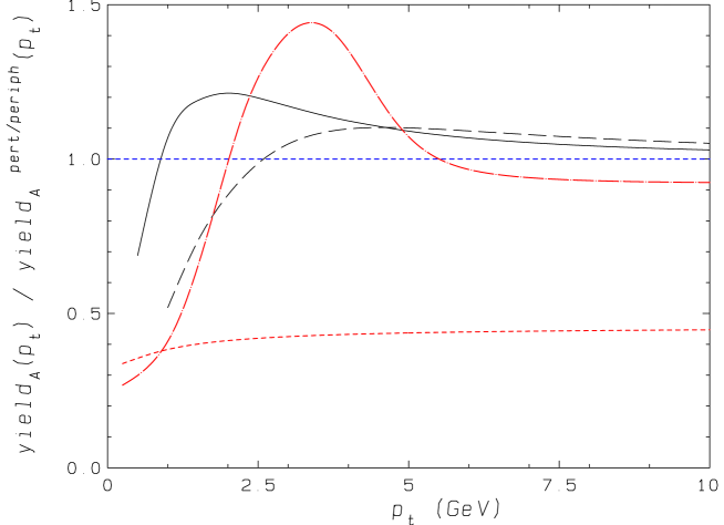
Figure 6: The gluon yield produced in p-A collisions, normalized to the perturbative yield for the MV gluon and to the peripheral yield for the evolved gluon distributions. The different curves are for the quasi-classical expression (27) normalized to (29) (dashed curve), the $k_{t}$-factorized spectrum with MV gluon (solid curve), and with evolved gluon distributions (10) (dot-dashed curve) and Eq.  (13) (short-dashed curve), respectively.

In order to compare with the perturbative behavior, we calculate for central rapidity $y=0$ the asymptotic limit of (27),

$$\frac{d\sigma^{pA}}{d^{2}p_{t}\ dy\ d^{2}b}\Bigg{|}_{{p_{t}}\gg Q_{s}}=\frac{4\alpha_{s}^{3}\ C_{F}}{\pi}\ K\ (2R\rho)\,\frac{1}{p_{t}^{4}}\,(\ln[\frac{p_{t}^{2}}{4\Lambda_{\rm QCD}^{2}}]+2\gamma_{E}-1)\,.$$ (29)

In the limit of small momenta, we quote  [5]

$$\frac{d\sigma^{pA}}{d^{2}p_{t}\ dy\ d^{2}b}\Bigg{|}_{{p_{t}}\ll Q_{s}}=\frac{\alpha_{s}\ C_{F}}{\pi^{2}}\ \frac{1}{p_{t}^{2}}\,,$$ (30)

which is obtained for ”frozen”, i.e. constant $Q_{s}$. We use Eq. (29) as the baseline for comparison for the MV gluon. For the evolved gluon we calculate the yield using the standard factorized formula. We take the proton distribution in the same functional shape as that of the nucleus, i.e. Eq. (10) and Eq. (13) with $\hat{Q}_{s}=\Lambda_{QCD}$. We compare the central yield ($\rho_{\rm part}=3.1\,{\rm fm^{-2}}$) to the peripheral yield ($\rho_{\rm part}=0.35\,{\rm fm^{-2}}$). Results are plotted in Fig.6.

For moderate momenta, i.e. above about twice the saturation scale $Q_{s}\simeq 1.4~{}{\rm GeV}$, the full rate for the MV gluon shows a Cronin-type enhancement with respect to the perturbative one. For small momenta $p_{t}\leq Q_{s}$, there is significant suppression, which can be immediately deduced when comparing (30) with (29). A qualitatively similar behavior is found when calculating the gluon spectrum from the factorized ansatz (2). As in the case of the nucleus-nucleus collisions, we find also that in p-A collisions the Cronin ratio in the evolved case depends strongly on the properties of the evolved distribution above the scaling window.

5 Conclusion

In summary, our study illustrates that quantitative results depend largely on the precise model-dependent implementation of saturation effects. A generic qualitative feature for the multiple scattering situation is that perturbative saturation leads to Cronin-type transverse momentum broadening of the produced gluon spectrum in both nucleus-nucleus and proton(deuteron)-nucleus collisions. In the evolved case there is an overall enhancement of the production yield relative to the perturbative baseline. The spectrum also exhibits strong transverse momentum broadening due to relatively large anomalous dimension. On the other hand, the absence or presence of the Cronin effect strongly depends on the behavior of the distribution function outside the scaling window. At present the shape of the evolved distribution in this momentum range is not known analytically. The recent numerical study  [17] strongly indicates that crossover from the scaling regime to the perturbative one is very slow and gradual, and that the Cronin effect which is present in the MV gluon is wiped out by the quantum evolution at high energies. Thus, $\phi_{A}^{\rm NLES}$ in Eq. (13) seems to provide a more realistic parametrization of the evolved gluon distribution than $\phi_{A}^{\rm NLEF}$ in Eq. (10).

Although the centrality dependence of the produced gluon spectrum shows $N_{\rm part}$ scaling in some limiting case, it can differ significantly from a simple $N_{\rm part}$ or $N_{\rm coll}$ scaling in the experimentally accessible regime depending on the shape of the gluon distribution .

A detailed comparison of perturbative saturation models to data not only requires the knowledge of the distribution and the improvement of the calculation of the gluon production yield beyond the factorized expression (2) used in this paper. It also requires the inclusion of fragmentation functions for gluons into pions, and a discussion of their possible medium-dependence [4].

On the qualitative level however we observe that the gluon distributions which lead to the Cronin effect in d-Au collisions also lead to the Cronin enhancement in the Au-Au collisions. And vice versa, if no Cronin effect appears in Au-Au, none is seen in d-Au collisions. Given the recent experimental observation of the Cronin enhancement in d-Au collisions at RHIC  [18] this supports the view that significant final state (“quenching”) effects are needed in order to account for the Au-Au data  [19].

Note added. When preparing the revised version of this paper we were made aware of  [20] and  [21] which also study the effects of saturation on the Cronin enhancement. These references agree with our results regarding the MV gluon. Regarding the evolved gluon, the detailed numerical study is reported in  [17].

Acknowledgments

The authors thank the Institute for Nuclear Theory at the University of Washington for its hospitality and the Department of Energy for partial support during the completion of this work. We thank A. H. Mueller for clarifying remarks and important suggestions when revising this work. We also thank E. Levin for asking the right questions. Useful discussions with N. Armesto, Y. Kovchegov, P. Jacobs, C. A. Salgado and D. Schiff are gratefully acknowledged. R. B. is supported, in part, by DFG, contract FOR 329/2-1. A. K. is supported by PPARC Advanced Fellowship.

References

- [1] D. Kharzeev and M. Nardi, Phys. Lett. B 507 (2001) 121 [arXiv:nucl-th/0012025], D. Kharzeev and E. Levin, Phys. Lett. B 523 (2001) 79 [arXiv:nucl-th/0108006], D. Kharzeev, E. Levin and M. Nardi, arXiv:hep-ph/0111315.
- [2] D. Kharzeev, E. Levin and L. McLerran, Phys. Lett. B 561 (2003) 93 [arXiv:hep-ph/0210332].
- [3] R. Baier, A. H. Mueller, D. Schiff and D. T. Son, Phys. Lett. B 502 (2001) 51 [arXiv:hep-ph/0009237].
- [4] E. Wang and X. N. Wang, Phys. Rev. Lett. 89 (2002) 162301 [arXiv:hep-ph/0202105], C. A. Salgado and U. A. Wiedemann, Phys. Rev. Lett. 89 (2002) 092303 [arXiv:hep-ph/0204221] and arXiv:hep-ph/0302184.
- [5] Y. V. Kovchegov and A. H. Mueller, Nucl. Phys. B 529 (1998) 451 [arXiv:hep-ph/9802440].
- [6] A. Kovner and U. A. Wiedemann, Phys. Rev. D 64 (2001) 114002 [arXiv:hep-ph/0106240] and arXiv:hep-ph/0304151.
- [7] L. V. Gribov, E. M. Levin and M. G. Ryskin, Phys. Rept. 100 (1983) 1.
- [8] L. D. McLerran and R. Venugopalan, Phys. Rev. D 49 (1994) 2233 [arXiv:hep-ph/9309289] and Phys. Rev. D 49 (1994) 3352 [arXiv:hep-ph/9311205].
- [9] Y. V. Kovchegov, Phys. Rev. D 54 (1996) 5463 [arXiv:hep-ph/9605446].
- [10] J. Jalilian-Marian, A. Kovner, L. D. McLerran and H. Weigert, Phys. Rev. D 55 (1997) 5414 [arXiv:hep-ph/9606337].
- [11] A. H. Mueller, Nucl. Phys. B 643 (2002) 501 [arXiv:hep-ph/0206216].
- [12] F. Gelis and J. Jalilian-Marian, Phys. Rev. D 67 (2003) 074019 [arXiv:hep-ph/0211363].
- [13] K. Golec-Biernat and M. Wusthoff, Phys. Rev. D 59 (1999) 014017 [arXiv:hep-ph/9807513].
- [14] I. Balitsky, Nucl. Phys. B 463 (1996) 99 [arXiv:hep-ph/9509348]; J. Jalilian-Marian, A. Kovner, A. Leonidov and H. Weigert, Phys. Rev. D 59 (1999) 014014 [arXiv:hep-ph/9706377]; J. Jalilian-Marian, A. Kovner and H. Weigert, Phys. Rev. D 59 (1999) 014015 [arXiv:hep-ph/9709432]; Y. V. Kovchegov, Phys. Rev. D 60 (1999) 034008 [arXiv:hep-ph/9901281].
- [15] E. Iancu, K. Itakura and L. McLerran, Nucl. Phys. A 708 (2002) 327 [arXiv:hep-ph/0203137] and arXiv:hep-ph/0212123; E. Iancu and R. Venugopalan, arXiv:hep-ph/0303204.
- [16] Y. V. Kovchegov and K. Tuchin, Phys. Rev. D 65 (2002) 074026 [arXiv:hep-ph/0111362].
- [17] J. Albacete et al.; arXiv:hep-ph/0307179.
- [18] S. S. Adler et al. [PHENIX Coll.], arXiv:nucl-ex/0306021; J. Adams [STAR Coll.], arXiv:nucl-ex/0306024; B. B. Back et al. [PHOBOS Coll.], arXiv:nucl-ex/0306025; I. Arsene et al. [BRAHMS Coll.], arXiv:nucl-ex/0307003.
- [19] K. Adcox et al. [PHENIX Collaboration], Phys. Rev. Lett. 88 (2002) 022301 [arXiv:nucl-ex/0109003], C. Adler et al. [STAR Collaboration], Phys. Rev. Lett. 89 (2002) 202301 [arXiv:nucl-ex/0206011], S. S. Adler et al. [PHENIX Collaboration], arXiv:nucl-ex/0304022, J. Adams [STAR Collaboration], arXiv:nucl-ex/0305015, B. B. Back et al. [PHOBOS Collaboration], arXiv:nucl-ex/0302015.
- [20] D. Kharzeev, Y. V. Kovchegov and K. Tuchin, arXiv:hep-ph/0307037.
- [21] J. Jalilian-Marian, Y. Nara and R. Venugopalan, arXiv:nucl-th/0307022.