The 3-D O(4) universality class and the phase transition in two-flavor QCD

Abstract:

We determine the critical equation of state of the three-dimensional O(4) universality class. We first consider the small-field expansion of the effective potential (Helmholtz free energy). Then, we apply a systematic approximation scheme based on polynomial parametric representations that are valid in the whole critical regime, satisfy the correct analytic properties (Griffiths’ analyticity), take into account the Goldstone singularities at the coexistence curve, and match the small-field expansion of the effective potential. From the approximate representations of the equation of state, we obtain estimates of several universal amplitude ratios.

The three-dimensional O(4) universality class is expected to describe the finite-temperature chiral transition of quantum chromodynamics with two light flavors. Within this picture, the O(4) critical equation of state relates the reduced temperature, the quark masses, and the condensates around $T_{c}$ in the limit of vanishing quark masses.

1 Introduction

In the theory of critical phenomena continuous phase transitions can be classified into universality classes determined only by a few properties characterizing the system, such as the space dimensionality, the range of interaction, the number of components of the order parameter, and the symmetry. Renormalization-group theory predicts that critical exponents and scaling functions are the same for all systems belonging to a given universality class. Here we consider the three-dimensional O(4) universality class, which is characterized by a four-component order parameter, O(4) symmetry, and effective short-range interactions. A representative of this universality class is the lattice spin model

$${\cal H}=-J\sum_{<ij>}\vec{s}_{i}\cdot\vec{s}_{j}-\sum_{i}\vec{H}\cdot\vec{s}_{i},$$ (1)

where $\vec{s}_{i}$ are four-component unit spins and the summation is extended over all nearest-neighbor pairs $<ij>$. We are interested in the critical equation of state that relates the magnetization $\vec{M}\equiv{1\over V}\langle\sum_{i}\vec{s}_{i}\rangle$, the temperature $T$, and a uniform external (magnetic) field $\vec{H}$ near the critical point $T=T_{c}$ and $\vec{H}=0$. The three-dimensional O(4) model is relevant for the finite-temperature behavior of quantum chromodynamics (QCD) with two light-quark flavors. Using symmetry arguments, it has been argued that, if the finite-temperature transition is continuous, it should belong to the same universality class of the three-dimensional O(4) vector model (1) [1, 2, 3].

The thermodynamics of quarks and gluons described by QCD is characterized by a transition from a low-temperature hadronic phase, in which chiral symmetry is broken, to a high-temperature phase with deconfined quarks and gluons (quark-gluon plasma), in which chiral symmetry is restored. The main features of this transition depend crucially on the QCD parameters, such as the number $N_{f}$ of flavors and the quark masses. Our qualitative understanding of the deconfinement transition is essentially based on the expected symmetry-breaking pattern that has been discussed at length in the light- [1, 2, 3, 4] and in the heavy- [5] quark regime. For recent reviews see, e.g., Refs. [6, 7, 8, 9, 10, 11]. In the limit of infinitely heavy quarks, i.e. in the pure SU(3) gauge theory, the order parameter for the transition is the Polyakov loop. The corresponding effective theory turns out to be a three-dimensional $Z_{3}$-symmetric spin model, which is expected to undergo a first-order transition. With decreasing the quark masses, the first-order transition should persist up to a critical surface (a line if only two quarks are considered) in the quark-mass phase diagram, where the transition becomes continuous and is expected to be Ising-like [1]. When the quark masses are further decreased, the phase transition disappears and one only observes an analytic crossover. In the opposite limit, i.e. for vanishing quark masses, we expect again a phase transition that is essentially related to the restoring of the chiral symmetry. Its nature can be argued by using symmetry arguments. In the chiral limit, since the axial $U(1)_{A}$ symmetry is broken by the anomaly, the relevant global symmetry group is expected to be $SU(N_{f})_{L}\times SU(N_{f})_{R}$. At $T=0$ the symmetry is spontaneously broken to $SU(N_{f})_{L+R}$ with $N_{f}^{2}-1$ Goldstone particles (pions and kaons). With increasing $T$, QCD is expected to undergo a chiral symmetry-restoring transition, where the order parameter is played by the expectation value of the quark bilinear $M^{i}_{j}=\langle\bar{q}^{i}_{L}q_{Rj}\rangle$. In the case the chiral symmetry-restoring phase transition is of first-order type, it persists also for nonvanishing masses, up to a critical surface in the quark-mass phase diagram where the transition becomes continuous and is expected to be Ising-like [4]. Outside this surface, i.e. for larger quark masses, the phase transition disappears and we are back in the analytic-crossover region discussed above. In the case the phase transition is continuous, its universal critical behavior can be described by an effective three-dimensional theory. Moreover, an analytic crossover is expected for nonvanishing quark masses, since the quark masses act as a external field coupled to the order parameter.

In the two-flavor case, $N_{f}=2$, the symmetry-breaking pattern of the transition is equivalent to $O(4)\rightarrow O(3)$. According to universality arguments, if two-flavor QCD undergoes a continuous transition, its critical behavior at $T_{c}$ should be that of the three-dimensional O(4) universality class. Since the quark masses act as an external (magnetic) field, a quark-mass term smooths out the singularity and instead of the transition one observes an analytic crossover, as in the O(4) model for nonvanishing magnetic field. In the small quark-mass regime the universal features of this analytic crossover can be still described by the scaling O(4) theory. However, universality arguments do not exclude that the transition is of first order. In this case, it would appear even for small nonvanishing masses. A first-order transition should be expected if the breaking of the axial $U(1)_{A}$ symmetry is effectively weak at $T_{c}$. Indeed, in the absence of the $U(1)_{A}$ axial anomaly, the symmetry breaking pattern is $U(2)_{L}\times U(2)_{R}\rightarrow U(2)_{L+R}$. The corresponding effective three-dimensional Landau-Ginzburg-Wilson theory [1] does not have stable fixed points, and therefore one expects a first-order transition. Since a first-order transition is generally robust under perturbations, for a sufficiently small breaking of the axial $U(1)_{A}$ symmetry at $T_{c}$ the transition should maintain its first-order nature. This issue has been investigated on the lattice, see, e.g., Refs. [13, 14, 15]. The $U(1)_{A}$ symmetry is not restored at $T_{c}$ and the transition is apparently of second order.

In the case of three light flavors, $N_{f}=3$, on the basis of the symmetry arguments reported above, it has also been argued that the transition is of first order, up to a critical surface in the quark-mass phase diagram, where it becomes continuous and it is expected to be in the Ising universality class [4]. This picture has been also supported by a recent Monte Carlo simulation [17]. See, e.g., Ref. [8] for a discussion of the phase diagram for generic values of the quark masses. A similar behavior has been put forward for $N_{f}>3$ [1].

Since many years the finite-temperature behavior of QCD has been investigated by numerical Monte Carlo simulations exploiting the lattice formulation of QCD. The available results are substantially consistent with the above-reported picture based on symmetry and universality, see, e.g., Refs. [18, 19, 20, 21, 22, 23]. However, although the evidence for a continuous transition in two-flavor QCD at $T_{c}\approx 172$ MeV is rather convincing (see, e.g., Refs. [18, 21]), conclusive evidence in favor of an O(4) scaling behavior in the continuum limit has not been achieved yet.

An accurate determination of the universal features of three-dimensional O(4) systems, such as the critical equation of state, is important to achieve an unambigous identification of the universality class of the finite-temperature transition in two-flavor QCD. Moreover, assuming that two-flavor QCD undergoes a continuous transition belonging to the three-dimensional O(4) universality class, the O(4) critical equation of state gives the asymptotic relations, for $T\rightarrow T_{c}$ and in the limit of vanishing quark masses, among the reduced temperature $t\equiv T/T_{c}-1$, the quark masses, and the expectation value of the bilinear $M^{i}_{j}=\langle\bar{q}^{i}_{L}q_{Rj}\rangle$. In particular, in the two-flavor case the relevant order parameter can be written as a four-component vector $\vec{\varphi}$, whose expectation value $\vec{M}$ is related to the quark condensate $\langle\bar{q}q\rangle$, and which is coupled to a uniform external field $\vec{H}$ related to the quark masses [1, 2, 3, 6]. The scaling properties can be written as

$$\vec{M}=B_{c}\vec{H}|H|^{(1-\delta)/\delta}E(y),$$ (2)

$$y=(B/B_{c})^{1/\beta}t|H|^{-1/(\beta+\gamma)},$$

where $\beta$, $\gamma$, and $\delta$ are the critical exponents, $B$ and $B_{c}$ are nonuniversal constants fixing the normalizations (they are the amplitudes of the magnetization at the coexistence curve and along the critical isotherm, respectively), and $E(y)$ is a universal function. Similar asymptotic relations can also be written for the (quark-mass) susceptibilities; they can be easily derived by taking appropriate derivatives of the relation (2). Corrections to the scaling behavior (2) are suppressed by powers of $t$ and $|H|$. The leading ones are of order $t^{\Delta}$ on the axis $H=0$ and of order $|H|^{\Delta/(\beta+\gamma)}$ on the critical isotherm [in general corrections have the scaling behavior $t^{\Delta}g(y)$], where $\Delta\approx 0.58$ [24, 25].

The critical equation of state of $O(N)$ models has already been studied in $\epsilon\equiv 4-d$ expansion at two loops [27] and in $1/N$ expansion at order $1/N$ [28]. However, these results do not allow us to obtain a quantitatively accurate determination of the critical equation of state, essentially because the available expansions are too short. On the other hand, on the numerical side, rather accurate results have been obtained from Monte Carlo simulations of the O(4) spin model (1) [29, 30, 31].

In this paper we compute the critical equation of state by using a different analytic method. The starting point is the small-field expansion of the effective potential (in statistical-mechanics language it corresponds to the small-magnetization expansion of the Helmholtz free energy), or equivalently of the equation of state, in the symmetric (high-temperature) phase ($t>0$). The first few nontrivial terms of this expansion have already been determined by exploiting field-theoretical methods in the continuum $\varphi^{4}$ theory [32, 33]. We use them to determine approximations of the equation of state that are valid in the whole critical regime. This requires an analytic continuation from the high-temperature phase ($t>0$) to the the coexistence curve ($t<0$), which can be achieved by using parametric representations [34, 35, 36, 37] implementing in a rather simple way the known analytic properties of the equation of state (Griffiths’ analyticity). We construct systematic approximation schemes based on polynomial parametric representations of the critical equation of state that have the correct analytic properties, take into account the Goldstone singularities at the coexistence curve, and match the known small-field behavior of the effective potential. Using the results for the critical equation of state, we then derive estimates of several universal amplitude ratios. As we shall see, we will provide rather accurate determinations of the scaling functions related to the magnetization, the longitudinal (quark-mass) susceptibility, and of several universal amplitude ratios, involving also quantitites defined at the so-called pseudo-critical line that corresponds to the maximum of the longitudinal susceptibility at fixed $H$.

The paper is organized as follows. In Sec. 2 we discuss the general properties of the critical equation of state. In particular, we consider the small-field expansion of the effective potential and of the critical equation of state in the symmetric phase. In Sec. 3 we describe our approximation schemes based on polynomial parametric representations, and determine the scaling functions that give the scaling behavior of the magnetization (quark condensate) and of the longitudinal susceptibility. Finally, in Sec. 4 we determine several universal amplitude ratios.

2 The critical equation of state

2.1 General properties

The equation of state relates the magnetization $\vec{M}$, the magnetic field $\vec{H}$, and the reduced temperature $t\equiv(T-T_{c})/T_{c}$. In the neighborhood of the critical point $t=0$, $H=0$, it is usually written in the scaling form

$$\vec{H}=B_{c}^{-\delta}\vec{M}M^{\delta-1}f(x),\qquad x\equiv t(M/B)^{-1/\beta},$$ (3)

where $M\equiv|\vec{M}|$, $f(x)$ is a universal scaling function normalized in such a way that $f(-1)=0$, $f(0)=1$, and $B_{c}$ and $B$ are the amplitudes of the magnetization on the critical isotherm and at the coexistence curve:

$$M=B_{c}H^{1/\delta},\qquad t=0,$$ (4)

$$M=B(-t)^{\beta},\qquad t<0,\quad H\rightarrow 0.$$ (5)

The scaling function $f(x)$ and $E(y)$, cf. Eq. (2), are clearly related:

$$E(y)=f(x)^{-1/\delta},\qquad y=xf(x)^{-1/(\beta+\gamma)}.$$ (6)

The equation of state is analytic for $|H|>0$, and therefore $f(x)$ is regular everywhere for $x>-1$. In particular, $f(x)$ has a regular expansion in powers of $x$ around $x=0$

$$f(x)=1+\sum_{n=1}^{\infty}f_{n}^{0}x^{n},$$ (7)

and a large-$x$ expansion of the form

$$f(x)=x^{\gamma}\sum_{n=0}^{\infty}f_{n}^{\infty}x^{-2n\beta}.$$ (8)

At the coexistence curve, i.e. for $x\rightarrow-1$, the Goldstone singularities appear. General arguments predict that, at the coexistence curve and in three dimensions, transverse and longitudinal susceptibilities behave respectively as

$$\chi_{T}={M\over H},\qquad\qquad\chi_{L}={\partial M\over\partial H}\sim H^{-1/2}.$$ (9)

In particular, the singularity of $\chi_{L}$ for $t<0$ and $H\to 0$ is governed by the zero-temperature infrared-stable Gaussian fixed point [28, 38, 39], leading to the prediction

$$f(x)\approx f_{2}^{\rm coex}\,(1+x)^{2}\qquad\qquad{\rm for}\qquad x\rightarrow-1.$$ (10)

The nature of the corrections to the behavior (10) is less clear. It has been conjectured [40, 41, 39], using essentially $\epsilon$-expansion arguments, that, for $x\to-1$, i.e., near the coexistence curve, $v\equiv 1+x$ has a double expansion in powers of $w\equiv HM^{-\delta}$ and $w^{(d-2)/2}$. This would imply that in three dimensions $f(x)$ could be expanded in integer powers of $v$ at the coexistence curve. On the other hand, an explicit calculation [42] to next-to-leading order in the $1/N$ expansion shows the presence of logarithms in the asymptotic expansion of $f(x)$ for $x\rightarrow-1$, so that $f(x)$ cannot be expanded in powers of $v$. However, these nonanalytic terms represent small corrections of order $O(v^{2}\log v)$ compared to the leading behavior (10).

Finally, beside the scaling functions $E(y)$ and $f(x)$, we introduce a scaling function associated with the longitudinal susceptibility, by writing

$$\chi_{L}=B_{c}|H|^{1/\delta-1}D(y),$$ (11)

where

$$D(y)={1\over\delta}\left[E(y)-{y\over\beta}E^{\prime}(y)\right]={\beta f(x)^{1-1/\delta}\over\beta\delta f(x)-xf^{\prime}(x)}.$$ (12)

The function $D(y)$ has a maximum at $y=y_{\rm max}$ corresponding to the crossover or pseudocritical line $t_{\rm max}(H)$, see also Sec. 4.

2.2 The small-field expansion of the effective potential

Let us consider the continuum $\varphi^{4}$ theory that describes the three-dimensional O(4) universality class, i.e.

$$S=\int d^{3}x\Bigl{\{}{1\over 2}\partial_{\mu}\vec{\varphi}(x)\cdot\partial_{\mu}\vec{\varphi}(x)+{1\over 2}{r}\,\vec{\varphi}(x)\cdot\vec{\varphi}(x)+{1\over 4!}u\left[\vec{\varphi}(x)\cdot\vec{\varphi}(x)\right]^{2}-\vec{H}\cdot\vec{\varphi}(x)\Bigr{\}},$$ (13)

where $\vec{\varphi}(x)$ is a four-component real field. Let us also consider a zero-momentum renormalization scheme [43] (see also Refs. [34, 44]):

$$\Gamma^{(2)}_{ab}(p)=\delta_{ab}Z_{\varphi}^{-1}\left[m^{2}+p^{2}+O(p^{4})\right],$$ (14)

$$\Gamma^{(4)}_{abcd}(0)=Z_{\varphi}^{-2}m{g\over 3}\left(\delta_{ab}\delta_{cd}+\delta_{ac}\delta_{bd}+\delta_{ad}\delta_{bc}\right),$$ (15)

where $\Gamma^{(n)}_{a_{1},\ldots,a_{n}}$ are $n$-point one-particle irreducible correlation functions, $m$ and $g$ are the zero-momentum mass scale and quartic coupling, respectively.

The effective potential (Helmholtz free energy) is related to the (Gibbs) free energy of the model. If $\vec{M}\equiv\langle\vec{\varphi}\rangle$ one defines

$${\cal F}(M)=\vec{M}\cdot\vec{H}-{1\over V}\log Z(H),$$ (16)

where $Z(H)$ is the partition function and the dependence on the temperature is always understood in the notation. The effective potential ${\cal F}(M)$ is the generator of the zero-momentum one-particle irreducible correlation functions. In the high-temperature phase it admits an expansion around $M=0$:

$$\Delta{\cal F}\equiv{\cal F}(M)-{\cal F}(0)=\sum_{j=1}^{\infty}{1\over(2j)!}a_{2j}M^{2j}.$$ (17)

This expansion can be rewritten in terms of the expectation value of the renormalized field $\varphi_{r}(x)=Z_{\varphi}^{-1/2}\varphi(x)$, i.e. $\vec{M}_{r}\equiv\langle\vec{\varphi}_{r}\rangle$,

$$\Delta{\cal F}={1\over 2}m^{2}M_{r}^{2}+\sum_{j=2}m^{3-j}{1\over(2j)!}g_{2j}M_{r}^{2j}.$$ (18)

Note that $g_{4}$ is the renormalized coupling $g$ appearing in Eq. (15); its critical limit is the fixed point of the renormalization-group equations, that is the zero of the Callan-Symanzik $\beta$-function $\beta(g)\equiv m\partial g/\partial m$. The coefficients $g_{2j}$ approach universal constants (which we indicate with the same symbol) for $m\to 0$. By performing a further rescaling

$$M_{r}^{2}={m\over g_{4}}z^{2}$$ (19)

in Eq. (18), the effective potential can be written as

$$\Delta{\cal F}={m^{3}\over g_{4}}A(z),$$ (20)

where

$$A(z)={1\over 2}z^{2}+{1\over 4!}z^{4}+\sum_{j=3}{1\over(2j)!}r_{2j}z^{2j},$$ (21)

and

$$r_{2j}={g_{2j}\over g_{4}^{j-1}}\qquad\qquad j\geq 3.$$ (22)

The universal quantities $g_{4}$ and the first few $r_{2j}$ have been estimated by using field-theoretical methods. Fixed-dimension perturbative calculations provide the estimates $g_{4}=17.30(6)$ (from an analysis [24] of the six-loop expansion of $\beta(g)$ [45]), $r_{6}=1.81(3)$ (from an analysis [32] of the corresponding four-loop series [33]) and $r_{8}=0.456$ (three-loop series [33]), while $\epsilon$-expansion computations give [32] $g_{4}=17.5(3)$ (four-loop series), $r_{6}=1.780(8)$ and $r_{8}=0.2(4)$ (three-loop series). Other substantially less precise results and references can be found in Refs. [32].

Since $z\propto t^{-\beta}M$ where $t\equiv T/T_{c}-1\propto r-r_{c}$, the equation of state can be written in the form

$$\vec{H}={\partial{\cal F}(M)\over\partial\vec{M}}\propto{\vec{M}\over|M|}t^{\beta\delta}F(z),$$ (23)

with

$$F(z)\equiv{\partial A\over\partial z}=z+{1\over 6}z^{3}+\sum_{j=3}{1\over(2j-1)!}r_{2j}z^{2j-1}.$$ (24)

The two functions $f(x)$ and $F(z)$ are related:

$$z^{-\delta}F(z)=F_{0}^{\infty}f(x),\qquad\qquad z=z_{0}x^{-\beta},$$ (25)

where $z_{0}=(R_{4}^{+})^{1/2}$ is a universal constant, see Sec. 4. Because of Griffiths’ analyticity, ${\cal F}(M)$ has also a regular expansion in powers of $t$ for $|M|$ fixed. Therefore, $F(z)$ has the large-$z$ expansion

$$F(z)=z^{\delta}\sum_{k=0}F^{\infty}_{k}z^{-k/\beta}.$$ (26)

3 Parametric representations of the equation of state

3.1 Polynomial approximation schemes

In order to obtain a representation of the equation of state that is valid in the whole critical region, we need to extend analytically the expansion (21) to the low-temperature region $t<0$. For this purpose, we use parametric representations that implement the expected scaling and analytic properties. We set [46]

$$M = m_{0}R^{\beta}m(\theta),$$

$$t = R(1-\theta^{2}),$$

$$H = h_{0}R^{\beta\delta}h(\theta),$$ (27)

where $h_{0}$ and $m_{0}$ are normalization constants. The variable $R$ is nonnegative and measures the distance from the critical point in the $(t,H)$ plane, while the variable $\theta$ parametrizes the displacement along the lines of constant $R$. The functions $m(\theta)$ and $h(\theta)$ are odd and regular at $\theta=0$ and at $\theta=1$. The constants $m_{0}$ and $h_{0}$ can be chosen so that $m(\theta)=\theta+O(\theta^{3})$ and $h(\theta)=\theta+O(\theta^{3})$. The smallest positive zero $\theta_{0}$ of $h(\theta)$, which should satisfy $\theta_{0}>1$, corresponds to the coexistence curve, i.e., to $T<T_{c}$ and $H\to 0$. The parametric representation satisfies the requirements of regularity of the equation of state. Singularities can only appear at the coexistence curve (due, for example, to the logarithms discussed in Ref. [42]), i.e., for $\theta=\theta_{0}$. The mapping (27) is not invertible when its Jacobian vanishes, which occurs when

$$Y(\theta)\equiv(1-\theta^{2})m^{\prime}(\theta)+2\beta\theta m(\theta)=0.$$ (28)

Thus, parametric representations based on the mapping (27) are acceptable only if $\theta_{0}<\theta_{l}$, where $\theta_{l}$ is the smallest positive zero of the function $Y(\theta)$.

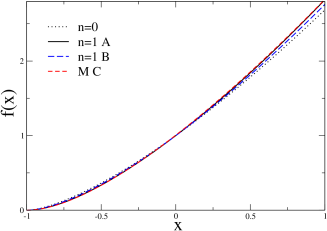
Figure 1: The scaling function $f(x)$ as obtained by the $n$=0, $n$=1 (A), and $n$=1 (B) approximations. For comparison, we also show the Monte Carlo (MC) result of Ref. [30], although it can be hardly distinguished from the $n$=1 (A) curve.

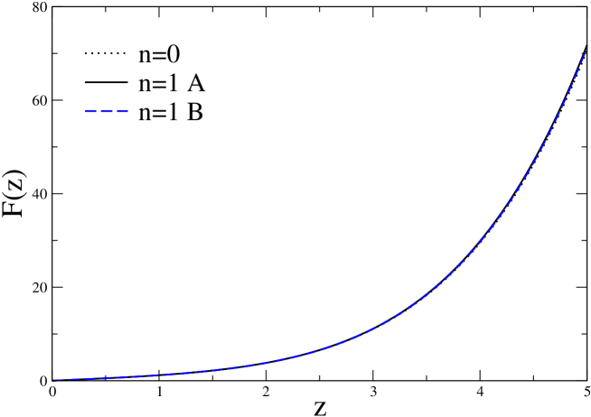
Figure 2: The scaling function $F(z)$.

The functions $m(\theta)$ and $h(\theta)$ are related to the scaling function $f(x)$ through

$$x={1-\theta^{2}\over\theta_{0}^{2}-1}\left[{m(\theta_{0})\over m(\theta)}\right]^{1/\beta},$$ (29)

$$f(x)=\left[{m(\theta)\over m(1)}\right]^{-\delta}{h(\theta)\over h(1)}.$$

The asymptotic behavior (10) is reproduced by requiring that

$$h(\theta)\sim\left(\theta_{0}-\theta\right)^{2}\qquad\qquad{\rm for}\qquad\theta\rightarrow\theta_{0}.$$ (30)

Following Ref. [37], we construct approximate polynomial parametric representations that have the expected singular behavior at the coexistence curve (Goldstone singularity) and match the known terms of the small-$z$ expansion of $F(z)$, cf. Eq. (24). We consider two distinct approximation schemes. In the first one, which we denote by (A), $h(\theta)$ is a fifth-order polynomial with a double zero at $\theta_{0}$ and $m(\theta)$ is a polynomial of order $(1+2n)$:

$${\rm scheme}\quad({\rm A}):\qquad\qquad m(\theta)=\theta\Bigl{(}1+\sum_{i=1}^{n}c_{i}\theta^{2i}\Bigr{)},$$ (31)

$$h(\theta)=\theta\left(1-\theta^{2}/\theta_{0}^{2}\right)^{2}.$$

In the second scheme, denoted by (B), we set

$${\rm scheme}\quad({\rm B}):\qquad\qquad m(\theta)=\theta,$$ (32)

$$h(\theta)=\theta\left(1-\theta^{2}/\theta_{0}^{2}\right)^{2}\Bigl{(}1+\sum_{i=1}^{n}c_{i}\theta^{2i}\Bigr{)}.$$

Here $h(\theta)$ is a polynomial of order $5+2n$ with a double zero at $\theta_{0}$. For $n$=0 approximations (A) and (B) coincide. It is worth noting that the $n$=0 approximation becomes exact in $O(N)$ models for $N\to\infty$ [28, 37]. In both schemes the parameter $\theta_{0}$ and the $n$ coefficients $c_{i}$ are determined by matching the small-$z$ expansion of $F(z)$. The scaling function $F(z)$ can be written in terms of the parametric representation as

$$z=\rho\,m(\theta)\left(1-\theta^{2}\right)^{-\beta},$$ (33)

$$F(z(\theta))=\rho\left(1-\theta^{2}\right)^{-\beta\delta}h(\theta),$$

where $\rho$ is a normalization [35, 26], which is fixed by matching the expansion (24) to order $z^{3}$. Explicitly, we have

$$\rho^{2}=6\beta(\delta-1)-{12\over\theta_{0}^{2}}-6bc_{1},$$ (34)

where $b=1,-1$ respectively for scheme (A) and (B). In both schemes, in order to fix $\theta_{0}$ and the $n$ coefficients $c_{i}$ we need to know the values of $n+1$ coefficients $r_{2j}$, i.e., $r_{6},...r_{6+2n}$. This method has been already applied to the determine the critical equation of state of the $XY$ [37, 47] and Heisenberg [48] universality classes.

3.2 Results

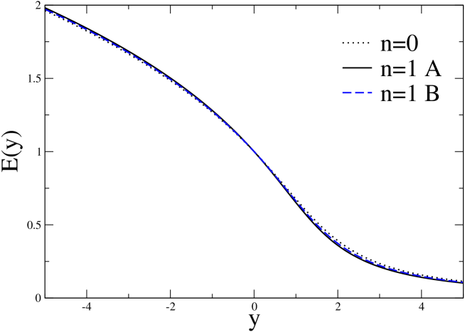
Figure 3: The scaling function $E(y)$.

In order to implement the above-presented approximation schemes, we use the Monte Carlo estimates [25] $\nu=0.749(2)$ and $\eta=0.0365(10)$ for the critical exponents, and the field-theoretical estimates $r_{6}=1.79(2)$ and $r_{8}=0.2(4)$ which take into account both fixed-dimension and $\epsilon$-expansion results, see Sec. 2.2. This will provide three different approximations: $n$=0, $n$=1 (A), and $n$=1 (B). We find

$$\theta_{0}^{2}=2.795(40)\qquad n=0,$$ (35)

and

$$\theta_{0}^{2}=2.949(150),\qquad c_{1}=-0.0225(200),\qquad n=1\;({\rm A}),$$ (36)

$$\theta_{0}^{2}=2.373(200),\qquad c_{1}=\phantom{-}0.0650(300),\qquad n=1\;({\rm B}),$$ (37)

where the number between parentheses indicates how much the coefficients vary when the input parameters change by one error bar. The relatively small value of $c_{1}$ in the $n$=1 approximations supports the effectiveness of the approximation schemes. In Figs. 1, 2, 3, and 4 we show respectively the scaling functions $f(x)$, $F(z)$, $E(y)$, $D(y)$, as obtained from the $n$=0, $n$=1 (A), and $n$=1 (B) approximations for the central values of the input parameters. The differences among the three approximations give an indication of the size of the systematic error of the approximation schemes. The figures show that it is rather small, suggesting that the $n=0,1$ representations already provide good approximations of the critical equation of state.

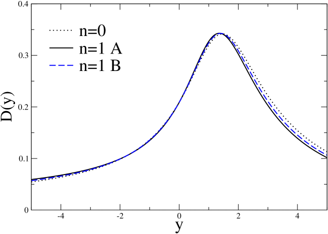
Figure 4: The scaling function $D(y)$.

In Fig. 1 we compare our results with the scaling function $f(x)$ obtained in Ref. [30] by interpolating Monte Carlo data for the O(4) spin model (1). The agreement is overall satisfactory. The Monte Carlo determination of $f(x)$ turns out to be hardly distinguishable from the $n$=1 (A) curve. A more direct comparison with the Monte Carlo data of Ref. [30] is presented in Fig. 5, where we plot $M/H^{1/\delta}$ versus $(J-J_{c})/H^{1/\beta\delta}$ using $\delta=4.789(6)$, $\beta=0.388(1)$ and the raw data reported there. To avoid finite-size and scaling corrections we only consider the results for the largest lattices that are closest to the critical point, in particular those satisfying $H\leq 0.01$ and $|J-J_{c}|<0.05$. The full line shown in Fig. 5 is the $n$=1 (A) approximation, cf. Eqs. (31) and (36), while the dotted lines show the uncertainty due to the error on the corresponding input parameters. The necessary normalization conditions related to the amplitudes $B$ and $B_{c}$, cf. Eq. (2), have been determined by fitting the data. The agreement is good: most Monte Carlo data are within the uncertainty of the $n$=1 (A) curve.

Table 1: Results concerning the scaling functions obtained by using the $n$=0, $n$=1 (A), and $n$=1 (B) approximations. Numbers marked with an asterisk are inputs, not predictions.

	$n=0$	$n=1$ (A)	$n=1$ (B)	final estimates
$f^{1}_{0}$	1.44(1)	1.53(9)	1.48(3)	1.50(8)
$f^{2}_{0}$	0.29(1)	0.35(6)	0.32(2)	0.33(5)
$f^{3}_{0}$	$-$0.060(4)	$-$0.08(1)	$-$0.07(1)	$-$0.08(2)
$f_{0}^{\infty}$	0.82(1)	0.92(10)	0.87(3)	0.89(9)
$f_{2}^{\rm coex}$	4.8(3)	2.2(1.3)	3.3(6)	2.8(1.4)
$r_{8}$	$-$0.3(1)	∗0.2(4)	∗0.2(4)
$r_{10}$	2.7(5)	$-$4(4)	$-$6(7)	$-$5(6)
$F_{0}^{\infty}$	0.0236(3)	0.0241(5)	0.0240(4)	0.0240(5)
$y_{\rm max}$	1.46(1)	1.35(10)	1.40(4)	1.38(9)
$D(y_{\rm max})$	0.3417(4)	0.3429(11)	0.3426(7)	0.3427(10)

In Table 1 we report results concerning the behavior of the scaling functions $f(x)$ and $F(z)$ for $H=0$ and on the critical isotherm, cf. Eqs. (7), (8), (10), (21), and (26). We also report estimates of $y_{\rm max}$ and $D(y_{\rm max})$, where $y_{\rm max}$ is the value of $y$ corresponding to the maximum of the scaling function $D(y)$ defined in Eq. (11). The displayed errors refer only to the uncertainty of the input parameters and do not include the systematic error of the procedure, which may be determined by comparing the results of the various approximations. Our final estimates are reported in the Table 1. They are obtained by taking the average of the results $n$=1 (A) and $n$=1 (B). The error is just indicative: it is the sum of the uncertainty induced by the input parameters (we take the average of the two errors) and of half of the difference between the two approximations. In most cases this procedure leads to an estimate that includes the $n$=0 result within its error. For comparison, we also report the estimates $f_{2}^{\rm coex}=2.20(5)$, $f_{0}^{\infty}=0.888(7)$, $F_{0}^{\infty}=0.018(4)$, $y_{\rm max}=1.33(5)$, and $D(y_{\rm max})=0.341(1)$, which can be obtained from the results of the fits of the Monte Carlo data reported in Refs. [30, 31]. Finally, we mention that the result for $r_{10}$ is consistent with the estimate $r_{10}=9(17)$ obtained from the analysis of its $O(\epsilon^{3})$ series [32].

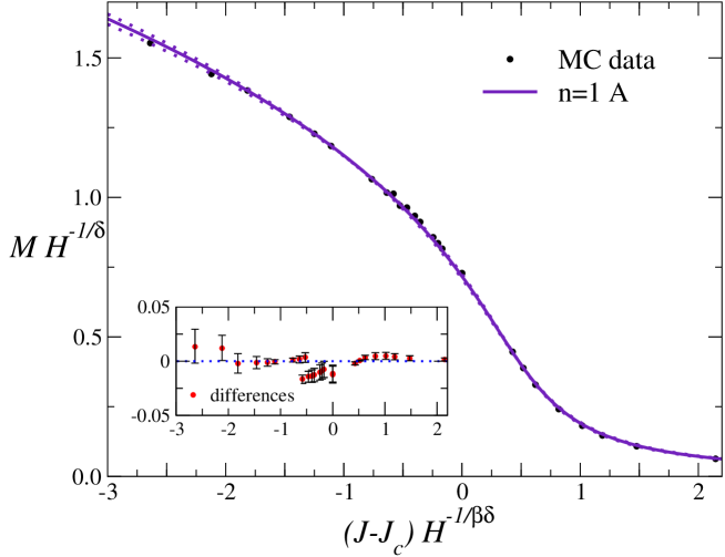
Figure 5: Monte Carlo data for $M/H^{1/\delta}$ versus $(J-J_{c})/H^{1/\beta\delta}$ from Ref. [30] compared with the $n$=1 (A) approximation (full line). The dotted lines show the uncertainty on the curve due to the errors on the input parameters. The inset shows the differences between the Monte Carlo data and the $n$=1 (A) curve: the errors are related to the uncertainty on the theoretical curve; the statistical errors of the Monte Carlo data are much smaller.

4 Universal amplitude ratios

Table 2: Definitions of several universal amplitude ratios.

Universal Amplitude Ratios
$U_{0}\equiv A^{+}/A^{-}$	$R_{c}^{+}\equiv\alpha A^{+}C^{+}/B^{2}$
$R_{4}^{+}\equiv-C_{4}^{+}B^{2}/(C^{+})^{3}$	$R_{\chi}\equiv C^{+}B^{\delta-1}/B_{c}^{\delta}$
$g_{4}\equiv-C_{4}^{+}/[(C^{+})^{2}(f^{+})^{3}]$	$Q^{+}\equiv\alpha A^{+}(f^{+})^{3}$
$R^{+}_{\xi}\equiv(Q^{+})^{1/3}$	$Q_{c}\equiv B^{2}(f^{+})^{3}/C^{+}$
$P_{m}\equiv{T_{p}^{\beta}B/B^{c}}$	$R_{p}\equiv{C^{+}/C_{p}}$

Universal amplitude ratios characterize the critical behavior of thermodynamic quantities that do not depend on the normalizations of the external (magnetic) field, of the order parameter (magnetization), and of the temperature. From the scaling function $f(x)$ one may derive many universal amplitude ratios involving zero-momentum quantities, such as the specific heat, the magnetic susceptibility, etc…. For example, the universal ratio of the specific-heat amplitudes in the two phases can be written as

$${A^{+}\over A^{-}}={\varphi(\infty)\over\varphi(-1)}$$ (38)

where, in the case of the O(4) universality class for which $-1<\alpha<0$,

$$\varphi(x)={x|x|^{\alpha-2}f^{\prime}(0)\over\alpha-1}+{|x|^{\alpha}f^{\prime\prime}(0)\over\alpha}-|x|^{\alpha-2}f(x)+\int_{0}^{x}dy\,|y|^{\alpha-2}\left[f^{\prime}(y)-f^{\prime}(0)-yf^{\prime\prime}(0)\right].$$ (39)

Several universal amplitude ratios can be expressed in terms of the amplitudes derived from the singular behavior of the specific heat

$$C_{H}=A^{\pm}|t|^{-\alpha}+b,$$ (40)

where $b$ is a nonuniversal constant, the magnetic susceptibility in the high-temperature phase

$$\chi=NC^{+}t^{-\gamma}$$ (41)

with $N=4$, the zero-momentum four-point connected correlation function in the high-temperature phase

$$\chi_{4}={N(N+2)\over 3}C_{4}^{+}t^{-\gamma-2\beta\delta}$$ (42)

(again with $N=4$), the second-moment correlation length in the high-temperature phase, corresponding to the inverse mass in the zero-momentum renormalization scheme, cf. Eqs. (14) and (15),

$$\xi=f^{+}t^{-\nu},$$ (43)

the spontaneous magnetization on the coexistence curve, cf. Eqs. (4) and (5). We also consider amplitudes along the crossover line $t_{\rm max}(H)$, that is defined as the reduced temperature where the longitudinal magnetic susceptibility $\chi_{L}(t,H)=\partial M/\partial H$ has a maximum at $H$ fixed, i.e.

$$t_{\rm max}(H)=T_{p}H^{1/(\gamma+\beta)},$$ (44)

$$\chi_{L}(t_{\rm max},H)=C_{p}t_{\rm max}^{-\gamma}.$$ (45)

In Table 2 we report the definitions of several universal amplitude ratios that have been considered in the literature. Their expressions in terms of the functions $m(\theta)$ and $h(\theta)$ can be found in Ref. [48]. Note the following relations

$$f_{0}^{\infty}=R_{\chi}^{-1},\qquad f_{1}^{\infty}={R_{4}^{+}\over 6R_{\chi}},$$ (46)

$$y_{\rm max}=P_{m}^{1/\beta},\qquad D(y_{\rm max})=R_{p}^{-1}P_{m}^{1-\delta}R_{\chi}.$$ (47)

where $f_{0}^{\infty}$ and $f_{1}^{\infty}$ are related to the large-$x$ behavior of $f(x)$, cf. Eq. (8), and $y_{\rm max}$ is the value of $y$ where the scaling function $D(y)$ takes its maximum.

In Table 3 we report the estimates of several universal amplitude ratios, as derived by using the approximations $n$=0, $n$=1 (A), and $n$=1 (B). Again, the displayed errors refer only to the uncertainty of the input parameters. Our final estimates are determined as in the case of the quantities reported in Table 1. They can be again compared with the Monte Carlo results reported in Refs. [30, 31]: $R_{\chi}=1.126(9)$, $R_{4}^{+}=8.6(9)$ and $P_{m}=1.11(2)$. There is good agreement, keeping again into account that Refs. [30, 31] used different values of the critical exponents (see footnote 6). Moreover, using Eq. (38) and the approximate interpolation formula of Refs. [30, 31] we obtain $U_{0}=2.0(2)$, where the error is obtained by varying the curve parameters within their error. We also mention the estimates [49] $U_{0}\approx 2.044$ and $R_{c}^{+}\approx 0.263$, obtained by an analysis of three-loop series in the minimal-subtraction scheme without $\epsilon$ expansion. They are in good agreement with those presented in Table 3.

Universal amplitude ratios involving the correlation-length amplitude $f^{+}$, such as $R_{\xi}^{+}$ and $Q_{c}$, can be obtained by using the estimate of $g_{4}$. If we take [24] $g_{4}=17.30(6)$, we obtain

$$R_{\xi}^{+}=\left({R_{c}^{+}R_{4}^{+}\over g_{4}}\right)^{1/3}=0.490(4),$$ (48)

$$Q_{c}={R_{4}^{+}\over g_{4}}=0.44(2).$$ (49)

Table 3: Estimates of several universal amplitude ratios.

	$n=0$	$n=1$ (A)	$n=1$ (B)	final estimates
$U_{0}$	2.03(3)	1.89(11)	1.93(6)	1.91(10)
$R_{c}^{+}$	0.250(5)	0.274(25)	0.263(9)	0.27(2)
$R_{4}^{+}$	8.04(7)	7.5(5)	7.7(2)	7.6(4)
$R_{\chi}$	1.22(2)	1.09(12)	1.15(4)	1.12(11)
$P_{m}$	1.159(3)	1.12(3)	1.140(11)	1.13(2)
$R_{p}$	2.049(3)	2.041(7)	2.042(6)	2.042(7)
$R_{c}^{+}\,R_{4}^{+}$	2.01(4)	2.05(5)	2.03(3)	2.04(5)

- [1] R.D. Pisarsky and F. Wilczek, Phys. Rev. D 29 (1984) 338.
- [2] F. Wilczek, Int. J. Mod. Phys. A 7 (1992) 3911.
- [3] K. Rajagopal and F. Wilczek, Nucl. Phys. B 399 (1993) 395.
- [4] S. Gavin, A. Gocksh, and R.D. Pisarski, Phys. Rev. D 49 (1994) 3079 [hep-ph/9311350].
- [5] B. Svetitsky and L.G. Yaffe, Nucl. Phys. B 210 (1982) 423.
- [6] K. Rajagopal, in Quark-Gluon Plasma 2, edited by R. Hwa (World Scientific, Singapore, 1995) [hep-ph/9504310].
- [7] F. Wilczek, hep-ph/0003183.
- [8] F. Karsch, in Lectures on Quark Matter, Proceedings of the 40th Internationale Universitätswochen für Kern- und Teilchenphysik, Lecture Notes in Physics 583, edited by W. Plessas and L. Mathelisch (Springer, Berlin, 2002) p. 209 [hep-lat/0106019].
- [9] J.B. Kogut, hep-lat/0209054.
- [10] E. Laermann and O. Philipsen, hep-ph/0303042.
- [11] D. H. Rischke, nucl-th/0305030.
- [12] A. Butti, A. Pelissetto, and E. Vicari, in preparation.
- [13] C. Bernard et al., Phys. Rev. Lett. 78 (1997) 598 [hep-lat/9611031].
- [14] J.B. Kogut, J.-F. Lagaë, and D.K. Sinclair, Phys. Rev. D 58 (1998) 054504 [hep-lat/9801020].
- [15] P.M. Vranas, Nucl. Phys. 83 (Proc. Suppl.) (2000) 414 [hep-lat/9911002].
- [16] M.C. Birse, T.D. Cohen, and J.A. McGovern, Phys. Lett. B 388 (1996) 137 [hep-ph/9608255]; Phys. Lett. B 399 (1997) 263 [hep-ph/9701408].
- [17] F. Karsch, E. Laermann, and C. Schmidt, Phys. Lett. B 520 (2001) 41 [hep-lat/0107020].
- [18] A. Ali Khan et al. (CP-PACS Collaboration), Phys. Rev. D 63 (2001) 034502 [hep-lat/0008011]; Phys. Rev. D 64 (2001) 074510 [hep-lat/0103028].
- [19] Y. Iwasaki, K. Kanaya, S. Kaya, and T. Yoshié, Phys. Rev. Lett. 78 (1997) 179 [hep-lat/9609022].
- [20] Y. Iwasaki, K. Kanaya, S. Sakai, and T. Yoshié, Z. Physik C 71 (1996) 343 [hep-lat/9504019].
- [21] F. Karsch, E. Laermann, and A. Peikert, Nucl. Phys. B 605 (2001) 579 [hep-lat/0012023].
- [22] J.B. Kogut and D.K. Sinclair, Phys. Rev. D 64 (2001) 034508 [hep-lat/0104011]; Phys. Lett. B 492 (2000) 228 [hep-lat/0005007].
- [23] C. Bernard, C. DeTar, S. Gottlieb, U.M. Heller, J. Hetrick, K. Rummukainen, R.L. Sugar, and D. Toussaint, Phys. Rev. D 61 (2000) 034503 [hep-lat/0002028].
- [24] R. Guida and J. Zinn-Justin, J. Phys. A 31 (1998) 8103 [cond-mat/9803240].
- [25] M. Hasenbusch, J. Phys. A 34 (2001) 8221 [cond-mat/0010463].
- [26] A. Pelissetto and E. Vicari, Phys. Rept. 368 (2002) 549 [cond-mat/0012164].
- [27] E. Brézin, D.J. Wallace, and K.G. Wilson, Phys. Rev. Lett. 29 (1972) 591; Phys. Rev. B 7 (1973) 232.
- [28] E. Brézin and D.J. Wallace, Phys. Rev. B 7 (1973) 1967.
- [29] D. Toussaint, Phys. Rev. D 55 (1997) 362 [hep-lat/9607084].
- [30] J. Engels and T. Mendes, Nucl. Phys. B 572 (2000) 289 [hep-lat/9911028].
- [31] J. Engels, S. Holtmann, T. Mendes, and T. Schulze, Phys. Lett. B 514 (2001) 299 [hep-lat/0105028].
- [32] A. Pelissetto and E. Vicari, Nucl. Phys. B 575 (2000) 579 [cond-mat/9911452]; Nucl. Phys. B 522 (1998) 605 [cond-mat/9801098]; Nucl. Phys. B 519 (1998) 626 [cond-mat/9711078].
- [33] A.I. Sokolov, E.V. Orlov, V.A. Ul’kov, and S.S. Kashtanov, Phys. Rev. E 60 (1999) 1344 [hep-th/9810082].
- [34] J. Zinn-Justin, Quantum Field Theory and Critical Phenomena, fourth edition (Clarendon Press, Oxford, 2001).
- [35] R. Guida and J. Zinn-Justin, Nucl. Phys. B 489 (1997) 626 [hep-th/9610223].
- [36] M. Campostrini, A. Pelissetto, P. Rossi, and E. Vicari, Phys. Rev. E 60 (1999) 3526 [cond-mat/9905078]; Phys. Rev. E 65 (2002) 066127 [cond-mat/0201180].
- [37] M. Campostrini, A. Pelissetto, P. Rossi, and E. Vicari, Phys. Rev. B 62 (2000) 5843 [cond-mat/0001440].
- [38] E. Brézin and J. Zinn-Justin, Phys. Rev. B 14 (1976) 3110.
- [39] I.D. Lawrie, J. Phys. A 14 (1981) 2489.
- [40] D.J. Wallace and R.P.K. Zia, Phys. Rev. B 12 (1975) 5340.
- [41] L. Schäfer and H. Horner, Z. Phys. B 29 (1978) 251.
- [42] A. Pelissetto and E. Vicari, Nucl. Phys. B 540 (1999) 639 [cond-mat/9805317].
- [43] G. Parisi, Cargèse Lectures (1973), J. Stat. Phys. 23 (1980) 49.
- [44] C. Itzykson and J.M. Drouffe, Statistical Field Theory (Cambridge Univ. Press, Cambridge, 1989).
- [45] G.A. Baker, Jr., B.G. Nickel, M.S. Green, and D.I. Meiron, Phys. Rev. Lett. 36 (1977) 1351. G.A. Baker, Jr., B.G. Nickel, and D.I. Meiron, Phys. Rev. B 17 (1978) 1365.
- [46] P. Schofield, Phys. Rev. Lett. 22 (1969) 606. B.D. Josephson, J. Phys. C: Solid State Phys. 2 (1969) 1114. P. Schofield, J.D. Litster, and J.T. Ho, Phys. Rev. Lett. 23 (1969) 1098.
- [47] M. Campostrini, M. Hasenbusch, A. Pelissetto, P. Rossi, and E. Vicari, Phys. Rev. B 63 (2001) 214503 [cond-mat/0010360].
- [48] M. Campostrini, M. Hasenbusch, A. Pelissetto, P. Rossi, and E. Vicari, Phys. Rev. B 65 (2002) 144520 [cond-mat/0110336].
- [49] H. Kleinert and B. Van den Bossche, Phys. Rev. E 63 (2001) 056113 [cond-mat/0011329].