Theory and phenomenology of non-global logarithms

We discuss the theoretical treatment of non-global observables, those quantities that are sensitive only to radiation in a restricted region of phase space, and describe how large ‘non-global’ logarithms arise when we veto the energy flowing into the restricted region. The phenomenological impact of non-global logarithms is then discussed, drawing on examples from event shapes in DIS and energy-flow observables in 2-jet systems. We then describe techniques to reduce the numerical importance of non-global logarithms, looking at clustering algorithms in energy flow observables and the study of associated distribution of multiple observables.

1 Introduction and Theory

Recently a distinction has been introduced between so-called global and non-global QCD observables. $\!{}^{{\bf?}}$ The former are sensitive to emissions in all directions, while the latter are sensitive only to emissions in some restricted angular region, for an example a jet or a hemisphere. Obvious examples of non-global (NG) observables are properties of individual jets (invariant mass, numbers of subjets). Many other common QCD observables are also non-global, including definitions of diffraction based on rapidity gaps (whether in terms of particles or energy flow); isolation criteria for photons (or other particles); distributions of interjet energy flow; or even the original Sterman-Weinberg jet definition. $\!{}^{{\bf?}}$

The question of globalness becomes of particular relevance whenever one places a severe restriction on the energy $E$ (or in some cases, transverse energy) flowing into the observed region. In such a situation the perturbative series develops logarithmically enhanced terms at all orders, at the very least single logs $\alpha_{s}^{n}\ln^{n}E/Q$, where $Q$ is the hard scale. For $E\ll Q$ such a series needs to be resummed. For global observables it has been shown $\!{}^{{\bf?}}$ that the resummation can be carried out to single logarithmic (SL) accuracy, essentially by using the approximation of independent emission off the underlying Born event.

Figure 1: Real and virtual contributions to the emission of gluon (2) from a $q{\bar{q}}g$ system.

Until recently it had universally been assumed $\!{}^{{\bf?}}$ that this approximation could be used more generally. However it turns out that for non-global observables, SL resummation is more subtle. $\!{}^{{\bf?}}$ This is illustrated in fig. 1, which shows left and right hemispheres ($\mathcal{H_{L}}$, $\mathcal{H_{R}}$) of a 2-jet $e^{+}e^{-}$ event, and two emissions going into opposite hemispheres such that $Q\gg E_{1}\gg E_{2}$. A global observable would for example measure the sum of the two gluon energies. Since $E_{1}\gg E_{2}$, placing a restriction $E_{\max}$ on the sum is equivalent to placing it directly on $E_{1}$ and there is cancellation between the real production and virtual loop contribution for gluon 2. Because of this cancellation, one is free to ‘mistreat’ the way gluon $2$ is emitted and pretend it is emitted from the simpler $q{\bar{q}}$ system, ignoring the presence of gluon $1$ — in other words one can make an independent emission approximation.

Now suppose we have an observable that measures the energy only in $\mathcal{H_{R}}$. The limit is placed just on gluon $2$, $E_{2}<E_{\max}$. On the other hand the loop contribution has an effective limit $E_{2,\mathrm{virtual}}\lesssim E_{1}$ and the mismatch between these two limits leads to a logarithmic enhancement $\ln E_{1}/E_{2}$. After integrating over $E_{1}$ one finds an overall contribution $\alpha_{s}^{2}\ln^{2}Q/E_{\max}$. Making an independent emission approximation, one would obtain the wrong coefficient for this term. The difference between the true answer (based on the coherent emission of gluon $2$ from the $q{\bar{q}}g_{1}$ system) and the independent emission result is termed a ‘non-global logarithm’ (NGL).

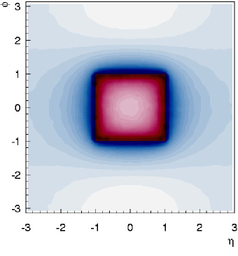
Figure 2: Contribution to the second order NGL for measurement in a square patch, shown as a function of rapidity and azimuth. Darker shades correspond to larger contributions.

At this two-gluon level, non-global logarithms are essentially an edge effect: it is only close to the boundary between measurement and non-measurement that one is sensitive to the difference between independent emission and the true two-gluon emission pattern. This is illustrated in figure 2 which shows (through the colour shading) the contribution to the NGL as a function of the two gluons’ rapidities $\eta$ and azimuths $\phi$ for the case in which the ‘measurement’ is carried out in a square patch $|\eta|<1$, $|\phi|<1$. One sees clearly that the largest contribution to the NG term is concentrated around the borders of the patch.

In the region where $\alpha_{s}\ln Q/E_{\max}$ is of order $1$, one needs to understand non-global effects at all orders $\alpha_{s}^{n}\ln^{n}Q/E_{\max}$. This amounts to accounting for the coherent radiation into the observed region of soft gluons from arbitrarily complex ensembles of harder (but still energy-ordered) gluons in the non-observed region. It turns out that given a naïve resummed calculation based on an independent emission picture, non-global effects can be accounted for by a multiplicative correction factor $\mathcal{S}(t)$, where $t$ is the running-coupling generalisation of $\frac{\alpha_{s}}{2\pi}\ln Q/E_{\max}$:

$$t=\int_{E_{\max}}^{Q}\frac{dE_{t}}{E_{t}}\frac{\alpha_{s}(E_{t})}{2\pi}\,.$$ (1)

It is sometimes useful also to write the expansion of $\mathcal{S}$, $\mathcal{S}(t)=\sum_{i=2}^{\infty}\,\mathcal{S}_{i}\,t^{i}$, and for example the two-gluon contribution discussed above gives us $\mathcal{S}_{2}$. The higher order terms are more difficult to calculate because of the complicated colour structures that appear for emission from multi-gluon configurations, and also because of the geometry. The colour problem has so far only been partially solved: using the large-$N_{c}$ approximation one can restrict one’s attention to planar graphs, equivalent to considering emission from sets of independent colour dipoles. $\!{}^{{\bf?}}$

Figure 3: The function $\mathcal{S}(t)$ for different geometries of observed region in a two-jet event. Slices are defined as containing all azimuths but a restricted range of rapidity.

Figure 4: Above: forbidding coherent radiation from an unobserved region (grey gluons) into the observed region (black gluons with crosses); below: schematic representation of the actual distribution of gluons in $\eta$ and $\phi$ (observed region is hashed).

Two equivalent approaches have been proposed to deal with the geometry dependence. In practice, the simplest way of solving the problem of the geometry dependence is through a Monte Carlo branching algorithm, $\!{}^{{\bf?}}$ in which the original $q{\bar{q}}$ dipole branches into two dipoles $qg$ and $g{\bar{q}}$. As one increases the logarithm $t$ each new dipole can itself branch and one iteratively builds up an ensemble of energy-ordered gluons with the correct (large-$N_{c}$) angular distribution. This algorithm is similar to that of the Ariadne event generator. $\!{}^{{\bf?}}$ One then determines $\mathcal{S}(t)$ by taking the number of events at scale $t$ that are free of emissions in the observed region and dividing it by the number of events that would have been expected on the basis of an independent emission picture.

Results for $\mathcal{S}(t)$ are shown in fig. 4 for various geometries of observed regions. From a theoretical point of view the most remarkable feature of these curves is that modulo normalisation, they all have the same $t$-dependence (in contrast, the fixed order $\mathcal{S}_{2}$ terms differ by more than a factor of two between the different geometries). The explanation proposed for this observation $\!{}^{{\bf?}}$ was so the so-called ‘buffer mechanism’, illustrated in fig. 4: the hypothesis is that the easiest way of forbidding ‘secondary’ emissions into the observed region is actually to forbid primary emissions close to the observed region. Accordingly for intermediate scales $t^{\prime}<t$ one finds a buffer region, free of emissions, surrounding the observed region. Larger differences $t-t^{\prime}$ imply a larger buffer region. As a result the dynamics governing the large-$t$ behaviour of $\mathcal{S}$ mostly occurs far from the observed the region and is not affected by the geometry of the observed region. Assuming that the buffer region is of size $\delta\eta_{\mathrm{buffer}}\simeq cC_{A}(t-t^{\prime})$ one comes to the conclusion that

$$\mathcal{S}(t)\sim e^{-2cC_{A}^{2}t^{2}}.$$ (2)

These arguments were placed on a mathematically sound footing by Banfi, Marchesini and Smye $\!{}^{{\bf?}}$. Firstly they introduced an alternative but equivalent approach to the problem of the geometry, in terms of a non-linear integral equation:

$$\partial_{t}\,\mathcal{S}_{ab}(t)=\int_{\mathrm{unmeasured}}\frac{d^{2}\Omega_{k}}{4\pi}\,w_{ab}(k)\left(U_{abk}^{(0)}(t)\,\mathcal{S}_{ak}(t)\,\mathcal{S}_{kb}(t)-\mathcal{S}_{ab}(t)\right),$$ (3)

where $\mathcal{S}_{ab}(t)$ is the non-global correction factor for a dipole $ab$, $w_{ab}(k)$ is the weight for emission of a soft gluon $k$ from $ab$ and $U^{(0)}_{abk}(t)$ accounts for the different ‘primary’ emission contributions for dipoles $ak,kb$ compared to dipole $ab$. They were then able to demonstrate the existence of scaling solutions to (3), proving the buffer mechanism, with $c$ evaluated numerically to be $2.5\pm 0.25\%$. They also evaluated a number of subleading corrections. They pointed out however that in practice (2) applies only for $t\gtrsim 0.5$, i.e. very asymptotic values of $t$. Phenomenologically, $t$ is limited to be $\lesssim 0.2$ and one should use the full solutions to $\mathcal{S}$.

1.1 Warnings for practitioners, a.k.a. Zoology

The definition of a non-global observable, given above, is one that is sensitive only to emissions (from the Born event) in a restricted angular region. However the situations in which NGLs can appear are rather subtle.

Firstly there exist observables that measure only a subset of the particles, but which nevertheless are global. An example is the heavy-hemisphere invariant squared mass in $e^{+}e^{-}$. Though only one hemisphere is measured, the observable is global because it is always the heavier hemisphere that is measured — in a situation such as fig. 1 the heavier hemisphere is always the one with the harder gluon (1) and one therefore never has the situation of a harder unobserved particle radiating into the observed region. Other examples include certain DIS event shapes (e.g. $B_{zE}$, $\tau_{zQ}$) where the measurement is carried out in one current hemisphere, but for which conservation of momentum causes an indirect sensitivity to emissions in the unobserved hemisphere. Such observables are known as indirectly global.

Another subtle case is that of observables referred to as discontinuously global. Such observables have different parametric sensitivities to emissions in different directions, e.g. $v\sim E_{t}^{2}/Q^{2}$ for emissions in one hemisphere, $v\sim E_{t}/Q$ for the other. Placing a limit on $v$ corresponds to different limits on $E_{t}$ in the two hemisphere (e.g. $\sqrt{v}Q$ and $vQ$ respectively) and one finds NGLs as for simple non-global observables, but with the appropriate replacement of the integration limits for $t$ in eq. (1). $\!{}^{{\bf?},{\bf?}}$

The most subtle situation is perhaps that of dynamically discontinuously global observables. These are observables which for a single emission appear global (typically indirectly global). However they involve non-linearities such that for the configurations of emissions that are most common (e.g. given a certain value of the observable) they develop different effective parametric dependence on emissions in different regions. $\!{}^{{\bf?}}$ One example of such an observable is the broadening $B_{zE}$ in DIS.

2 Phenomenological implications

In this section we will examine the phenomenological impact of NGLs in a variety of non-global observables. We will look at the invariant-squared jet mass in DIS $\!{}^{{\bf?}}$ (although the conclusions we draw will apply to $e^{+}e^{-}$ non-global event shapes as well) and at 2-jet energy flows. $\!{}^{{\bf?}}$ In both kinds of observable we will see that by neglecting the non-global logarithm suppression factor, one overestimates the distributions and cross sections by a considerable, and certainly phenomenologically relevant, amount.

2.1 NGLs in DIS and $e^{+}e^{-}$ event shapes

Event shapes (ES), and their distributions, $\!{}^{{\bf?}}$ are widely used to compare the predictions of perturbative QCD with experimental observation. As an example of a non-global event shape, we will use the DIS invariant squared jet mass $\rho$, defined as

$$\rho=\frac{\left(\Sigma_{\mathcal{H}_{C}}P_{i}\right)^{2}}{4\left(\Sigma_{\mathcal{H}_{C}}|\vec{P}_{i}|\right)^{2}},$$ (4)

where the summation is over all particles in the current-hemisphere ($\mathcal{H}_{C}$). When calculating the cross section for $\rho$ to be smaller than some given value, one finds that in the exclusive limit, small $\rho$, each power of the coupling is accompanied by up to two powers of $\ln\rho$, associated with with soft and collinear divergences. These terms need to be resummed. The standard accuracy is next-to-leading logarithmic, which in this case implies the inclusion of all single-logarithmic terms, i.e. the same accuracy as NG contributions.

In figure 6 we show the effect of the non-global logarithms on the resummed distribution for $\rho$. The broken line is the resummation without NGLs, and the solid line shows the result once they are included through the function $\mathcal{S}$ discussed above. Neglecting the non-global logarithms leads to an overestimation of the peak-height by around 40%, while the effect is smaller in other parts of the distribution. In practice, the resummed calculation is usually matched to a fixed-order calculation, which includes the NGLs to order $\alpha_{s}^{2}$ and so reduces the impact of neglecting the NGLs in the final result.

2.2 NGLs in 2 jet energy flow observables

Let us now examine the impact of non-global logarithms on energy flow observables. $\!{}^{{\bf?}}$ Such observables have attracted considerable interest in recent time as an infrared-safe way of studying gaps-between-jets processes $\!{}^{{\bf?}}$ and the underlying event in hadron-hadron collisions. $\!{}^{{\bf?}}$ We shall take as our observable the total amount of transverse energy flowing into a restricted region of phase space $\Omega$. The probability for the amount of transverse energy to be smaller than some value $Q_{\Omega}$ is

$$\Sigma_{\Omega}(Q_{\Omega})=\frac{1}{\sigma}\int_{0}^{Q_{\Omega}}d\,E_{t}\frac{d\sigma}{dE_{t}}\,.$$ (5)

As discussed in section 1 this can be written as the product of two contributions,

$$\Sigma_{\Omega}(Q_{\Omega})=\mathcal{S}(t)\times\Sigma_{P}(t)\,,$$ (6)

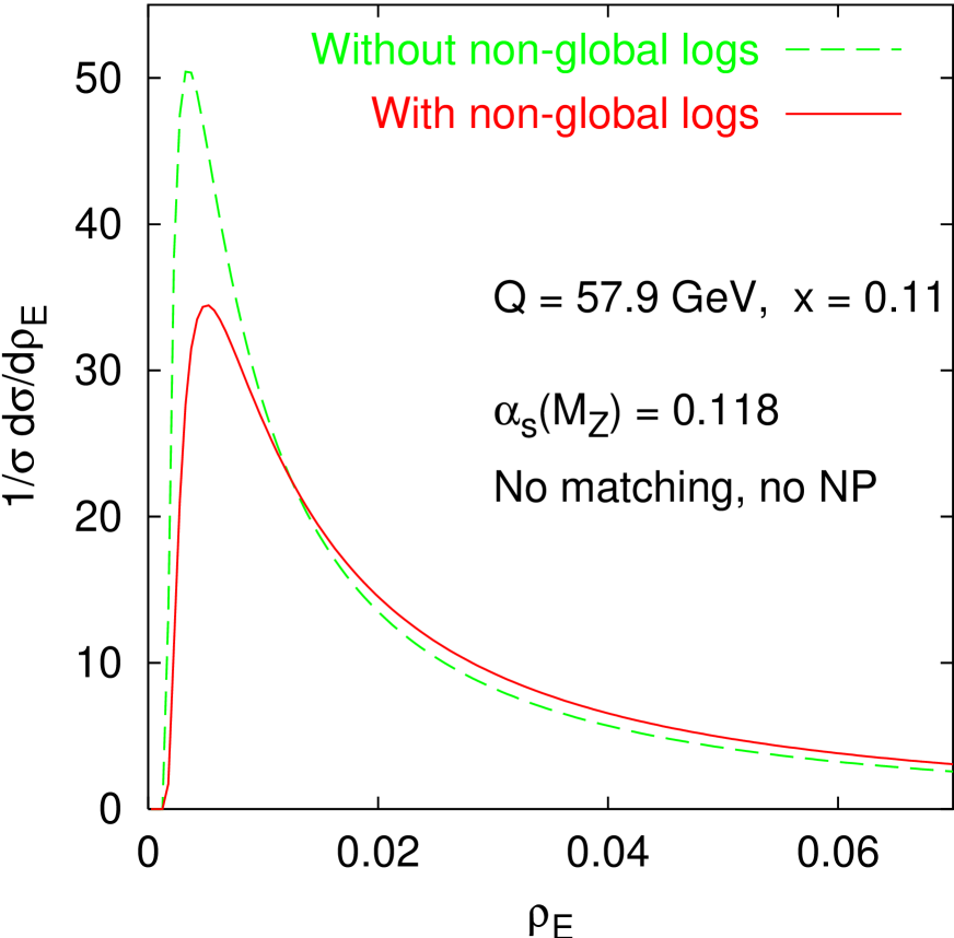
Figure 5: The impact of non-global logarithms (which enter at the NLL level) on a non-global DIS event shape.

Figure 6: The impact of non-global logarithms on the 2-jet energy flow observable $\Sigma_{\Omega}$. The upper plot shows the relation between $Q_{\Omega}$, $Q$ and $t$.

where the function $\Sigma_{P}$ is based on an independent gluon emission approximation (‘primary’ radiation into $\Omega$), while $\mathcal{S}(t)$ accounts for secondary coherently radiated emission into $\Omega$ and $t$ is defined as the integral of $\alpha_{s}/2\pi$ between $Q_{\Omega}$ and $Q$. We can understand the phenomenological implications of the non-global logarithms on this observable by comparing the result for $\Sigma_{\Omega}$, calculated with only primary emissions, with the full result for $\Sigma_{\Omega}$, which accounts also for non-global logarithms. We do this in figure 6, where $\Omega$ is a slice in rapidity of width $\Delta\eta=1.0$. The plot clearly show the phenomenological impact of the NGLs on this observable; the suppression is significant, particularly at larger values of the effective logarithm $t$. The typical energies of current colliders corresponds to about $t=0.15$ and if we take this as our reference value, the inclusion of non-global logarithms increases the suppression, relative to the primary-only case, by a factor of about 1.65. Similar results are found for other definitions of $\Omega$, for example a patch in phase space bounded in rapidity and azimuthal angle.

3 Controlling non-global logarithms

In this section we will describe ways of controlling, or taming, non-global logarithms. Such a study is important given that our methods for resumming NG logarithms are both approximate (large-$N_{C}$ limit) and cumbersome (numerical or asymptotic). We will look at two different approaches: minimising the numerical effect of the NGLs by clustering the final state, and also by examining associated distributions of pairs of observables.

3.1 Clustering algorithms

The application of clustering algorithms $\!{}^{{\bf?}}$ to the final state is motivated by recent H1 and ZEUS analyses $\!{}^{{\bf?}}$ of gaps-between-jets processes at HERA. In these analyses, the inclusive $k_{t}$ algorithm is used to define the hadronic final state, and hence the rapidity gap $\Omega$, and a gap event is defined by a restriction of the total transverse energy into $\Omega$. This observable, sensitive to soft radiation into $\Omega$ only, is clearly non-global, and so sensitive to non-global logarithmic effects. However, as we will show, the clustering procedure reduces the numerical importance of the NGLs for this observable, $\!{}^{{\bf?}}$ and we can see why by looking at how the $k_{t}$ clustering algorithm works. The essential feature is that in an iterative algorithm over all the final state particles, it merges particles of lower transverse momentum into particles with higher transverse momentum, to produce pseudo-particle or mini-jets. Consider applying this algorithm to two gluons with strongly ordered transverse momentum,

$$E_{T,1}\gg E_{T,2},$$ (7)

where gluon one, directed outside of the region $\Omega$, then in turn radiates gluon two into the region $\Omega$. The strong ordering ensures this configuration produces a non-global logarithm. When we cluster this system, gluon two will be clustered into, or merged with, gluon one (and hence pulled out of the gap) if the two gluons are sufficiently close in the $(\eta,\phi)$ plane,

$$(\eta_{1}-\eta_{2})^{2}+(\phi_{1}-\phi_{2})^{2}<R^{2},$$ (8)

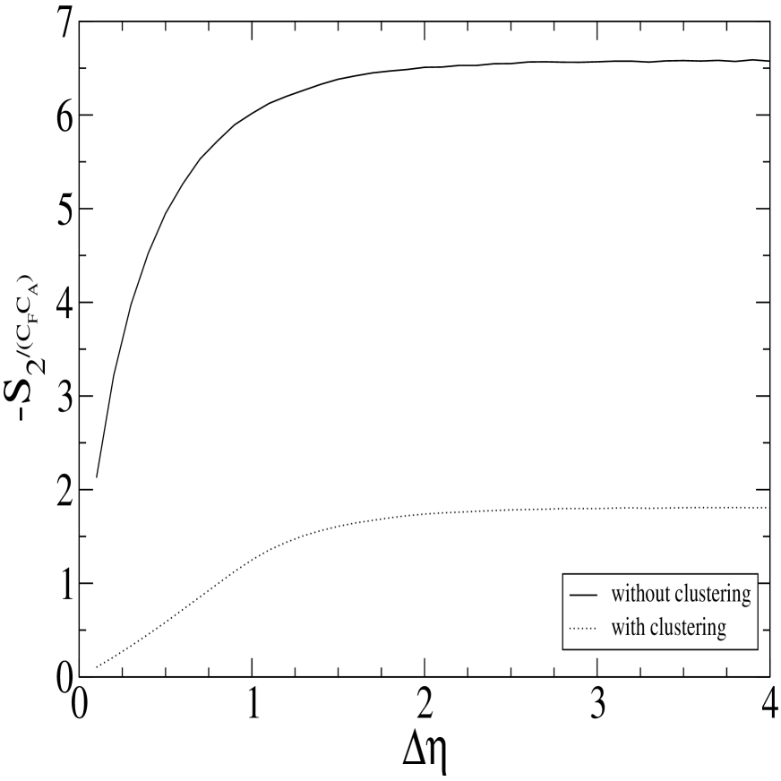
Figure 7: The leading, $\mathcal{S}_{2}$ contribution to the non-global logarithm function $\mathcal{S}(t)$, with and without clustering. The saturation of $S_{2}$ at high $\Delta\eta$ is seen for both the non-clustered and the clustered case, with a lower saturation value for the latter.

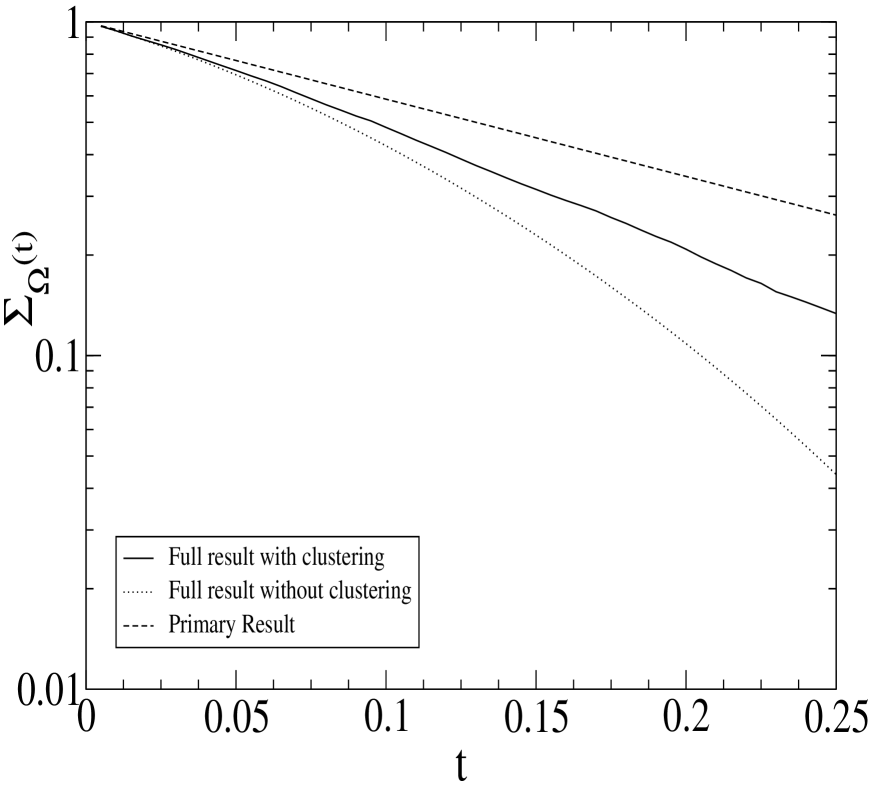
Figure 8: The phenomenological impact of the $k_{t}$ clustering procedure is to reduce the numerical importance of non-global logarithms on this 2-jet energy flow observable.

where $R$ is a parameter playing the role of a radius in the algorithm. Therefore to get a kinematical configuration which produces a NGL, the two gluons need to be sufficiently separated in the $(\eta,\phi)$ plane to avoid being merged. Hence the $k_{t}$ algorithm ‘cleans up’ the restricted region of phase space, $\Omega$, and pulls soft gluons out of the gap. Figure 8 shows the leading, $\mathcal{S}_{2}$ contribution (order $\alpha_{s}^{2}$) to the NGL function $\mathcal{S}(t)$, without clustering (solid line) and with clustering (broken line.) In both cases $\mathcal{S}_{2}$ rapidly saturates at high $\Delta\eta$, which results from the fact that the NGLs are an edge effect, and the saturation value for the clustered case is smaller than that of the non-clustered case. This follows from the fact that, although the clustering algorithm pulls gluons out of the gap, gluons can still be sufficiently separated in the $(\eta,\phi)$ plane to survive clustering and give a significant NGL contribution.

Figure 8 shows the all-orders calculation of the full function $\Sigma$, where $\Omega$ is taken to be a slice in rapidity of $\Delta\eta=1.0$. These figures allow us to see the phenomenological impact of the non-global logarithms on these observables, as they show the function $\Sigma_{P}$ (only primary logarithms) and the full function $\Sigma$ (primary and non-global logarithms) with and without clustering. We recall that $t$ is around $0.15$ to $0.2$ at the energies of current colliders, and as before we will take $t=0.15$ as our reference value. The plot shows that the non-global logarithms cause a considerable suppression of $\Sigma$, relative to the primary-only result, and that by clustering the final state this suppression is reduced. At $t=0.15$ the full result without clustering is suppressed relative to the primary only result by $1.65$, and this suppression is reduced with clustering to around $1.2$.

3.2 Event shape/Energy flow Correlations

Another way of reducing the phenomenological impact of NGLs that has been proposed, $\!{}^{{\bf?}}$ is the study of associated distributions in two variables. In this work, one combines measurement of a jet shape $V$ in the whole of phase space (for example thrust, $V=1-T$) and that of the transverse away-from-jets energy flow $E_{\mathrm{out}}$. The former is a global measurement and the latter is a non-global measurement. If the observable $V$ selects 2-jet-like configurations, one measures the associated distribution,

$$\Sigma_{\mathrm{2ng}}(Q,V,E_{out}),$$ (9)

where $Q$ is the hard scale. It has been shown that this distribution factorizes, $\!{}^{{\bf?}}$

$$\Sigma_{\mathrm{2ng}}(Q,V,E_{out})=\Sigma(Q,V)\cdot\Sigma_{\mathrm{out}}(VQ,E_{\mathrm{out}}),$$ (10)

where $\Sigma(Q,V)$ is the standard global distribution of $V$ and $\Sigma_{\mathrm{out}}(VQ,E_{\mathrm{out}})$ contains the logarithmic distribution in $E_{\mathrm{out}}$. This latter distribution, containing non-global logarithms is evaluated at the reduced scale $VQ$, and hence the logarithmic terms will be $(\alpha_{s}\log(VQ/E_{\mathrm{out}}))^{n}$. The work of Berger, Kúcs and Sterman $\!{}^{{\bf?}}$ considered the region in which $VQ$ and $E_{\mathrm{out}}$ were comparable, so that the NGLs give a negligible contribution. Thus, for a restricted subset of appropriately selected events, it is possible, to ‘tune out’ the non-global logarithmically enhanced terms in associated distributions.

4 Conclusion

To summarise, non-global logarithms are recently discovered contributions that arise in the distributions of any QCD observable sensitive only to emissions in a restricted part of phase space. They are phenomenologically important and significant progress has been made in resumming them to all orders in the large-$N_{c}$ limit. One of the main directions of current work focuses on understanding ways of designing observables so as to reduce the impact of non-global contributions.

References

References

- [1] M. Dasgupta and G. P. Salam, Phys. Lett. B 512 (2001) 323.
- [2] G. Sterman and S. Weinberg, Phys. Rev. Lett. 39 (1977) 1436.
- [3] S. Catani, L. Trentadue, G. Turnock and B. R. Webber, Nucl. Phys. B 407 (1993) 3.
- [4] For example in references 6, 10, 11 and 12 of M. Dasgupta and G. P. Salam, Acta Phys. Polon. B 33 (2002) 3311.
- [5] A. Bassetto, M. Ciafaloni and G. Marchesini, Phys. Rept. 100 (1983) 201.
- [6] L. Lönnblad, Comp. Phys. Comm. 71 (1992) 15.
- [7] M. Dasgupta and G. P. Salam, JHEP 0208 (2002) 032.
- [8] A. Banfi, G. Marchesini and G. Smye, JHEP 0208 (2002) 006.
- [9] Yu. L. Dokshitzer and G. Marchesini, JHEP 0303 (2003) 040.
- [10] M. Dasgupta and G. P. Salam, JHEP 0203 (2002) 017.
- [11] G. Oderda and G. Sterman, Phys. Rev. Lett. 81 (1998) 3591.
- [12] G. Marchesini and B.R. Webber, Phys. Rev. D 38 (1988) 3419.
- [13] S. Catani, Yu. L. Dokshitzer, M. H. Seymour and B. R. Webber, Nucl. Phys. B 406 (1993) 187.
- [14] C. Adloff et al. [H1 Collaboration], Eur. Phys. J. C 24 (2002) 517.
- [15] R. B. Appleby and M. H. Seymour, JHEP 0212 (2002) 063.
- [16] C. F. Berger, T. Kúcs and G. Sterman, hep-ph/0303051.