Pion production in deeply virtual Compton scattering

Abstract

Using a soft pion theorem based on chiral symmetry and a $\Delta(1232)$ resonance model we propose an estimate for the production cross section of low energy pions in the deeply virtual Compton scattering (DVCS) process. In particular, we express the $ep\to e\gamma\pi N$ processes in terms of generalized parton distributions. We provide estimates of the contamination of the $ep\to e\gamma p$ DVCS observables due to this associated pion production processes when the experimental data are not fully exclusive, for a set of kinematical conditions representative of present or planned experiments at JLab, HERMES and COMPASS.

I Introduction

The past few years have witnessed an intense theoretical activity in the field of Generalized Parton Distributions (GPDs). They parametrize the non perturbative content of the hadrons and are essentially matrix elements of the form Ji97b ; Rad96a

$$\left\langle N^{\prime}\left|\bar{q}_{\alpha}(x^{\mu})q_{\beta}(0)\right|N\right\rangle,$$ (1)

where $x^{\mu}$ is a light-like vector ($x^{2}=0)$. In (1) $q_{\alpha}$ is the quark field with Dirac index $\alpha$ and $N,\,N^{\prime}$ are two hadronic states which can differ either by their structure or by the kinematics. The limit $N=N^{\prime}$ gives the ordinary parton distributions.

In the Bjorken limit the GPDs appear in the amplitudes of exclusive reactions such as

$$\gamma^{*}(q)+N\rightarrow M+N^{\prime},$$ (2)

where $\gamma^{*}$ is a highly virtual photon ($Q^{2}=-q_{\mu}q^{\mu}\rightarrow\infty$ ) and $M$ can be a meson or a photon, in which case the reaction is called Deeply Virtual Compton Scattering (DVCS). It is widely believed that DVCS is conceptually the cleanest process to access the GPDs. The basic reason is that the amplitude for meson production involves the not so well known meson wave function. By contrast the final real photon in DVCS can be considered as pointlike because photon structure effects (VDM-like) are suppressed by powers of $1/Q^{2}$ Ji98a ; Rad98 ; Col99 .

This theoretical simplicity of DVCS is to some extent counterbalanced by its experimental difficulty which is certainly greater than in the case of meson production. Nevertheless a number of experimental attempts to measure photon electroproduction off the proton have been performed or are in progress Air02 ; Step02 ; Halla ; Compass ; H1zeus . For the interpretation of these experiments to be fruitful it is compulsory to have a control on the exclusivity of the final state. If we consider DVCS on the proton, the most interesting final state is the proton itself,

$$\gamma^{*}+p\rightarrow\gamma+p$$ (3)

and from now on we restrict our attention to this case. For further reference we call it “Elastic DVCS”.

The problem for most experiments is that the experimental energy resolution is not good enough to isolate the exclusive $(\gamma+p)$ channel because it is separated from the first strong inelastic channel by only the small pion mass. In practice such data will always be contaminated by the reactions, referred to as Associated DVCS (ADVCS) :

$$\gamma^{*}+p\rightarrow\gamma+p+\pi^{0}\,\,\,{\rm or}\,\,\gamma^{*}+p\rightarrow\gamma+n+\pi^{+},$$ (4)

where $\pi^{+,0}$ is a low energy pion which escapes detection. Note that experiments which have sufficient energy resolution to distinguish the $\gamma\pi N$ final state from the $\gamma p$ one can study the process (4) for itself Michel03 , thereby enlarging the scope of virtual Compton scattering. This is likely to be the case of the experiments planned at Jlab.

In this paper we propose a calculation of the cross section for reaction (4) and we compare it with the elastic channel (3) by integrating over the pion momentum up to a given cutoff. As the dangerous pions are those which have a small energy we use the soft pion techniques based on chiral symmetry. In the soft pion limit, that is $k_{\pi}\rightarrow 0$ where $k_{\pi}$ is the pion 4-momentum, this allows to evaluate the associated DVCS amplitude using the same generalized parton distribution as in the elastic case. So, in a relative sense, this evaluation is model independent. The inherent limitation of this approach is that, apart the chiral limit ($m_{\pi}\rightarrow 0$ ), it gives a reliable estimate only for a small center of mass (CM) energy of the final pion-nucleon pair. Typically the upper limit is set by the excitation energy of the first $\Delta$ resonance, that is about 300 MeV. In order to increase the range of validity of our estimate we propose a (model dependent) estimate of the associated DVCS corresponding to

$$\gamma*+p\rightarrow\gamma+\Delta.$$

For this we use the large $N_{c}$ limit as a guidance which allows one to relate the GPDs of the $N\rightarrow\Delta$ transition to the ones of the $N\rightarrow N$ transition Fra00 .

In practice one measures the $(l,\,l^{\prime},\,\gamma)$ reaction where $l$ denotes either a muon or an electron. The amplitude $T^{ll^{\prime}\gamma}$ for this reaction is the coherent sum of $T^{VCS}$, the virtual Compton scattering amplitude and of $T^{BH}$ the amplitude of the Bethe-Heitler process where the final photon is emitted by the lepton. When the reaction produces only a proton (elastic case) the calculation of this “elastic-BH” amplitude only involves the elastic form factors of the proton, which are well known. When a pion is produced together with the final nucleon, then the corresponding “associated-BH” (ABH) amplitude involves the pion electro-production amplitude. For consistency reasons we shall evaluate this amplitude in the same framework as the associated DVCS.

Our paper is organized as follows: in Section II we specify the kinematics and give the relevant expressions for the amplitudes and cross sections. In Section III we remind the leading order approximation for the DVCS amplitude and define the twist-2 quark operators which control the DVCS amplitude both in the elastic and associated case. In Section IV we remind the definition of the GPDs in the elastic case. In Section V we derive the soft pion theorems relevant for the evaluation of the associated DVCS and BH amplitudes. In Section VI we present a model to estimate the associated DVCS and BH in the $\Delta$ region. Section VII is devoted to a presentation and discussion of our results in kinematical situations of interest. Section VIII is our conclusion.

II Preliminary

Table 1: External particles variables.

	Initial	Final	Final	Initial	Final	Final
	lepton	lepton	photon	proton	nucleon	pion
Momentum	$k$	$k^{\prime}$	$q^{\prime}$	$p$	$p^{\prime}$	$k_{\pi}$
Mass	$m_{l}$	$m_{l}$	$0$	$M$	$M$	$m_{\pi}$
Helicity, spin	$h$	$h^{\prime}$	$\lambda^{\prime}$	$\sigma$	$\sigma^{\prime}$
Wave function	$u(k,h)$	$u(k^{\prime},h^{\prime})$	$\varepsilon^{\prime}(q^{\prime},\lambda^{\prime})$	$u(p,\sigma)$	$u(p^{\prime},\sigma^{\prime})$

In Table 1 we have collected the characteristics of the particles involved in the reaction. We define $q$ as the momentum of the virtual photon exchanged in the VCS process, that is $q=k-k^{\prime}$. So the BH virtual photon has $q-q^{\prime}$. The relevant Lorentz scalars are

$$Q^{2}=-q^{2},\,\,\,t_{\gamma}=(q-q^{\prime})^{2},\,\,\,x_{B}=\frac{Q^{2}}{2p.q},\,\,\,W^{2}=(p+q-q^{\prime})^{2}.$$ (5)

We shall also note $t=(p^{\prime}-p)^{2}$ which coincides with $t_{\gamma}$ in the elastic case or in the limit $k_{\pi}=0.$

Figure 1: Graph of the virtual Compton process

Figure 2: Graphs of the Bethe-Heitler process

In the one photon exchange approximation and in the Lorentz gauge we have the generic expressions for the VCS and BH amplitudes :

$$T^{VCS} = \pm e^{3}\varepsilon^{\prime*}_{\mu}H^{\mu\nu}\frac{1}{Q^{2}}\bar{u}(l^{\prime})\gamma_{\nu}u(l),$$ (6)

$$T^{BH} = -e^{3}\,J_{\nu}\,\frac{1}{t_{\gamma}}\,\bar{u}(l^{\prime})\left[\gamma.\varepsilon^{\prime*}\frac{1}{\gamma.(k^{\prime}+q^{\prime})-m_{l}}\gamma^{\nu}+\right.$$ (7)

$$\,\,\,\,\,\,\,\,\,\,\,\,\,\,\,\,\,\,\,\,\,\,\,\,\,\,\,\,\,\,\,\,\,\,\,\,\,\left.\gamma^{\nu}\frac{1}{\gamma.(k-q^{\prime})-m_{l}}\gamma.\varepsilon^{\prime*}\right]u(l)$$

$$T^{ll^{\prime}\gamma} = T^{VCS}+T^{BH}$$ (8)

They correspond to the graphs of Fig.1 and 2 respectively. In the above expressions the charge $e=\sqrt{4\pi/137}$ has been factored out and the $\pm$ sign refers to the charge of the lepton beam. The spinors are normalized to $\bar{u}u=2m$ with $m$ a generic mass and the photon polarisation is normalized to $\varepsilon^{\prime}.\varepsilon^{\prime}=-1$. The amplitudes $H$ and $J$ are defined by

$$H^{\mu\nu} = -i<f|\int d^{4}xe^{-iq.x}T\left[j^{\mu}(0),j^{\nu}(x)\right]|i>,$$ (9)

$$J^{\mu} = <f|j^{\mu}(0)|i>,$$ (10)

where $i,\,f$ are the appropriate hadronic states and $j(x)$ is the electromagnetic current carried by the quarks

$$j^{\mu}(x)=\bar{q}\gamma^{\mu}{\cal Q}q(x)=\sum_{f}{\cal Q}_{f}\bar{q}_{f}\gamma^{\mu}q_{f}(x),$$ (11)

with $\cal Q$ the diagonal charge matrix ${\cal Q}=[2/3,-1/3,\cdots]$. The matrix element of the electromagnetic current between nucleon states has the usual form factor decomposition :

$$<N(p^{\prime})|j^{\mu}(0)|N(p)>=\bar{u}(p^{\prime})\left[F_{1}^{p,n}(t)\gamma^{\mu}+iF_{2}^{p,n}(t)\frac{\sigma^{\mu\nu}(p^{\prime}-p)_{\nu}}{2M}\right]u(p)$$ (12)

where $p,n$ refer to the proton or the neutron and $t=(p-p^{\prime})^{2}$. With our normalizations we have $F_{1}^{p}(0)=1,\,F_{1}^{n}(0)=0,\,F_{2}^{p}(0)=1.79,\,F_{2}^{n}(0)=-1.91$.

We shall note $T^{ll^{\prime}\gamma}_{el.}$ the amplitude for a final hadronic state containing only a proton and $T^{ll^{\prime}\gamma}_{as.}(\pi^{+,0})$ the amplitude for producing a nucleon and a pion of charge +1 or 0. A similar notation will be used for the cross sections.

To fix the idea, we consider an experiment where $(k^{\prime},q^{\prime})$ the momenta of the final lepton and photon are measured while the final hadronic state $p^{\prime}$ or $(p^{\prime},k_{\pi})$ is not observed. The elastic $(ll^{\prime}\gamma)$ event is selected by the missing mass condition

$$W^{2}=(k-k^{\prime}+p-q^{\prime})^{2}=M^{2}.$$ (13)

In pratice the events will be integrated up to a cutoff $W_{max}$ which generally exceeds the pion production threshold. In the following we assume that the experimental resolution on $W$ is nevertheless good enough so that the production of more than one pion can be neglected.

If we assume that the one particle states are normalized as :

$$<k|k^{\prime}>=(2\pi)^{3}2k_{0}\delta(\vec{k}-\vec{k}^{\prime}),$$ (14)

we have the following expressions for the invariant cross sections :

$$d\sigma^{ll^{\prime}\gamma}_{el.} = d^{4}\Gamma\delta(W-M)dW\left|T^{ll^{\prime}\gamma}_{el.}\right|^{2},$$ (15)

$$d\sigma^{ll^{\prime}\gamma}_{as.}(\pi^{+,0}) = d^{4}\Gamma dW\frac{\left|\vec{k}^{*}_{\pi}\right|}{16\pi^{3}}\int d\hat{k}^{*}_{\pi}\left|T^{ll^{\prime}\gamma}_{as.}(\pi^{+,0})\right|^{2}.$$ (16)

In the above equations the common phase space factor is

$$d^{4}\Gamma=\frac{dx_{B}dQ^{2}dt_{\gamma}d\Phi}{128(2\pi)^{4}(p.k)^{2}x_{B}\sqrt{1+4M^{2}x_{B}^{2}/Q^{2}}}$$ (17)

where $\Phi$ is the angle between the planes $(\vec{k},\vec{k}\,^{\prime})$ and $(\vec{q},\vec{q}\,^{\prime})$ and $\vec{k}^{*}_{\pi}=\left|\vec{k}^{*}_{\pi}\right|\hat{k}^{*}_{\pi}$ stands for the pion momentum in the frame defined by $\vec{p}+\vec{q}-\vec{q}\,^{\prime}=0,$ that is the rest frame of the final pion-nucleon pair. One has

$$\left|\vec{k}^{*}_{\pi}\right|^{2}=\frac{W^{4}-2W^{2}(M^{2}+m_{\pi}^{2})+(M^{2}-m_{\pi}^{2})^{2}}{4W^{2}}.$$ (18)

From Eqs. (15,16) we see that the contamination of the elastic reaction by the associated one is measured by the dimensionless quantity

$$\kappa(Q^{2},x_{B},t_{\gamma},\Phi)=\frac{1}{16\pi^{3}}\frac{\int_{M+m_{\pi}}^{W_{max}}dW\left|\vec{k}^{*}_{\pi}\right|\int d\hat{k}^{*}_{\pi}\sum_{hel.}\left(\left|T^{ll^{\prime}\gamma}_{as.}(\pi^{+})\right|^{2}+\left|T^{ll^{\prime}\gamma}_{as.}(\pi^{0})\right|^{2}\right)}{\sum_{hel}\left|T^{ll^{\prime}\gamma}_{el.}\right|^{2}}.$$ (19)

where $\sum_{hel}$ denotes the sum over all the helicities. This is the quantity we want to evaluate.

III Handbag approximation for the VCS amplitude

We need to evaluate the hadronic tensor $H^{\mu\nu}$ (Eq.9) in the generalized Bjorken limit which here is defined by :

$$Q^{2}\rightarrow\infty,\,x_{B}\,{\rm fixed},\,t_{\gamma}/Q^{2}\rightarrow 0,\,W^{2}/Q^{2}\rightarrow 0,$$ (20)

where the two last conditions are necessary to have factorisation of the amplitude Col99 . The condition that $W$ remains small with respect to $Q$ is not explicitely stated for elastic VCS since $W=M$ in this case, but it is necessary for the associated VCS. The factorisation theorem garantees that the amplitude factorizes in a hard part which can be computed in perturbation theory as a series in $\alpha_{S}(Q^{2})$ and a soft part which depends on the long distance structure of the hadron. In this work we consider only the leading term of the hard part which amounts to evaluate the amplitude in the handbag approximation as shown in Fig. 3

Figure 3: The handbag approximation to the VCS amplitude. The crossed term is not shown.

For this purpose we adapt the formulation of Ji97b to our problem. In the Bjorken limit both the elastic and associated VCS are light-cone dominated. Therefore it is convenient to introduce two light-like vectors $\tilde{n}$ and $\tilde{p}$ to record the flow of hard momentum. These Sudakov vectors are chosen to be in the hyper-plane defined by the virtual photon momentum $q$ and another vector $P$ which is related to the target-ejectile motion. In our case it is convenient to choose :

$$P = \frac{p+p^{\prime}}{2}\,{\rm for\,\,the\,\,elastic\,\,VCS},$$ (21)

$$P = \frac{p+p^{\prime}+k_{\pi}}{2}\,{\rm for\,\,the\,\,associated\,\,VCS},$$ (22)

so that, for both reactions, $P$ has the same expression in terms of $p,\,q,\,q^{\prime}$ that is :

$$P=p+\frac{q-q^{\prime}}{2}=p+\frac{\Delta}{2}.$$ (23)

Other choices of $P$ are allowed, for instance $P=p$, but the formulation is more symmetric if one uses the definition (23). One imposes the normalization conditions :

$$\tilde{n}^{2}=\tilde{p}^{2}=0,\,\,\,\tilde{n}.\tilde{p}=1,\,\,\,\tilde{n}.P=1,$$ (24)

and one defines the variable $\xi^{\prime}$ as :

$$\xi^{\prime}=\frac{Q^{2}}{4P.q}=\frac{P.q}{2P^{2}}\left[-1+\sqrt{1+\frac{Q^{2}P^{2}}{\left(P.q\right)^{2}}}\right]\approx\frac{x_{B}/2}{1-x_{B}/2}{\rm\,\,in\,\,the\,\,Bjorken\,\,limit.}$$ (25)

From this one gets the decomposition :

$$P = \tilde{p}+\frac{P^{2}}{2}\tilde{n},$$

$$q = -2\xi^{\prime}\,\tilde{p}+\frac{Q^{2}}{4\xi^{\prime}}\tilde{n},$$ (26)

where

$$P^{2}=P^{\mu}P_{\mu}=\frac{M^{2}+W^{2}}{2}-\frac{t_{\gamma}}{4}.$$ (27)

An arbitrary vector $a$ has the covariant decomposition :

$$a=a.\tilde{n}\,\tilde{p}+a.\tilde{p}\,\tilde{n}+a(\bot),$$ (28)

with the $\bot$ component defined by $a(\bot).\tilde{n}=a(\bot).\tilde{p}=0$. If one restricts to the case where the final photon is real one then gets :

$$\Delta=-2\xi\tilde{p}+\left(\xi P^{2}+\frac{W^{2}-M^{2}}{2}\right)\tilde{n}+\Delta(\bot),$$

where :

$$\xi=\xi^{\prime}\frac{Q^{2}-t_{\gamma}-2\xi^{\prime}\,(W^{2}-M^{2})}{Q^{2}+4\xi^{\prime 2}P^{2}}\approx\xi^{\prime}{\rm\,\,in\,\,the\,\,Bjorken\,\,limit.}$$

If one keeps the leading light-cone singularity of the time ordered product of currents in Eq. (9) one has, at leading order in $\alpha_{s}(Q^{2})$ Ji97a  :

$$H^{\mu\nu}=\int dx\,C_{+}^{\mu\nu}(x,\xi)<f|\sum_{f}{\cal Q}_{f}^{2}S_{f}(x,\tilde{n})|i>$$

$$+\int dx\,C_{-}^{\mu\nu}(x,\xi)<f|\sum_{f}{\cal Q}_{f}^{2}S^{5}_{f}(x,\tilde{n})|i>+O\left(\frac{1}{Q}\right),$$ (29)

where the hard scattering coefficients (in which we consistently make the approximation $\xi\approx\xi^{\prime}$) write :

$$C_{+}^{\mu\nu}(x,\xi) = \frac{1}{2}(\tilde{n}^{\mu}\tilde{p}^{\nu}+\tilde{n}^{\nu}\tilde{p}^{\mu}-g^{\mu\nu})\left(\frac{1}{x-\xi+i\varepsilon}+\frac{1}{x+\xi-i\varepsilon}\right),$$ (30)

$$C_{-}^{\mu\nu}(x,\xi) = \frac{i}{2}\varepsilon^{\mu\nu\rho\sigma}\tilde{p}_{\rho}\tilde{n}_{\sigma}\left(\frac{1}{x-\xi+i\varepsilon}-\frac{1}{x+\xi-i\varepsilon}\right),$$ (31)

The twist-2 operators $S_{f}$ and $S_{f}^{5}$, for which we often use the global notation $S^{(5)}_{f}$ or $S^{(5)}$, are defined by :

$$S_{f}(x,\tilde{N}) = \int\frac{d\lambda}{2\pi}e^{i\lambda x}\bar{q}_{f}(-\lambda\tilde{N}/2)\gamma.\tilde{N}\,q_{f}(\lambda\tilde{N}/2),$$ (32)

$$S_{f}^{5}(x,\tilde{N}) = \int\frac{d\lambda}{2\pi}e^{i\lambda x}\bar{q}_{f}(-\lambda\tilde{N}/2)\gamma.\tilde{N}\,\gamma^{5}q_{f}(\lambda\tilde{N}/2)$$ (33)

with $\tilde{N}$ an arbitrary light-like vector. They obviously satisfy the scaling law :

$$S^{(5)}(\omega x,\omega\tilde{N})=S^{(5)}(x,\tilde{N}).$$ (34)

In Eq.(29) one has $\tilde{N}=\tilde{n}$, which is the only relic of the hard scattering in the soft matrix elements.

Figure 4: Representation of the twist-2 operator.

In Fig. 4 we have represented the matrix element of $S^{(5)}$ between generic hadronic states $i(p_{1})$ and $f(p_{2})$. The quark lines are on mass shell Fock states quantized at equal light cone time $x_{\mu}\tilde{N}^{\mu}=0.$ If one labels the momenta of the initial and final active quarks as $K-(p_{2}-p_{1})/2$ and $K+(p_{2}-p_{1})/2$ respectively, then the integration over $\lambda$ in Eqs. (32,33) implies that $x=K.\tilde{N}$. On the other hand, from the additivity of the longitudinal momentum, one has :

$$-\frac{\left|(p_{1}+p_{2}).\tilde{N}\right|}{2}\leq K.\tilde{N}\leq\frac{\left|(p_{1}+p_{2}).\tilde{N}\right|}{2},$$

So, if one chooses the normalization $\tilde{N}.(p_{1}+p_{2})/2=1$ as in (24), the integration over $x$ is effectively restricted to the interval $[-1,1]$ in Eq. (29).

In Eq. (29) the initial state is always the nucleon, with momentum $P-\frac{\Delta}{2}=p$. On the other hand the final state, which has momentum $P+\frac{\Delta}{2}=p+\Delta$, can be either the nucleon ($p+\Delta=p^{\prime}$) or the pion-nucleon system ($p+\Delta=p^{\prime}+k_{\pi}$). Note that for given $p,\,q,\,q^{\prime}$ the Sudakov vectors are the same in both cases. This is not essential but it simplifies the formulation.

Finally, we point out that because expression (29) is accurate up to terms of order $1/Q$ gauge invariance is not strictly satisfied. One finds instead :

$$q^{\prime}_{\mu}H^{\mu\nu}\sim\Delta(\perp),\,\,\,H^{\mu\nu}q_{\nu}=0.$$

However it has been shown in Vdh99 that electromagnetic gauge invariance is restored by adding to $H^{\mu\nu}$ a term which is explicitely of order $\sqrt{-t_{\gamma}}/Q$, and therefore does not contribute in the Bjorken limit. The effect of this extra term has been calculated for realistic situations and found to be negligibleVdh99 . So gauge invariance is not a serious issue as long as the conditions (20) are satisfied.

IV Generalized partons distributions for the elastic case

The matrix elements of $S^{(5)}$ are the non perturbative inputs of the calculation. If we note $N(p_{1}),N(p_{2})$ two generic nucleon states, the elastic matrix elements are parametrized according to Ji97b  :

$$<N(p_{2})|S_{f}(x,\tilde{N})|N(p_{1})>=$$

$$\frac{1}{P_{12}.\tilde{N}}\bar{u}(p_{2})\left[H_{f/N}\gamma.\tilde{N}+iE_{f/N}\frac{\sigma^{\mu\nu}\tilde{N}_{\mu}(p_{2}-p_{1})_{\nu}}{2M}\right]u(p_{1}),$$ (35)

$$<N(p_{2})|S_{f}^{5}(\kappa,\tilde{N})|N(p_{1})>=$$

$$\frac{1}{P_{12}.\tilde{N}}\bar{u}(p_{2})\left[\tilde{H}_{f/N}\gamma.\tilde{N}+\tilde{E}_{f/N}\frac{\tilde{N}.(p_{2}-p_{1})}{2M}\right]\gamma^{5}u(p_{1}),$$ (36)

where we note $P_{12}=(p_{1}+p_{2})/2.$ The Generalized Parton Distributions (GPDs) $H,\,E,\,\tilde{H},\,\tilde{E}$ are a priori functions of $x$ and of the invariants which can be formed with $p_{1},\,p_{2}$ and $\tilde{N}$, that is :

$$GPD=GPD\left\{x,\,(p_{2}-p_{1}).\tilde{N},\,P_{12}.\tilde{N},\,t_{12}=(p_{1}-p_{2})^{2}\right\}.$$

However from the scaling law (34) and the definitions (35,36) we have :

$$GPD\left\{\omega x,\,\omega(p_{2}-p_{1}).\tilde{N},\,\omega P_{12}.\tilde{N},\,t_{12}\right\}=GPD\left\{x,\,(p_{2}-p_{1}).\tilde{N},\,P_{12}.\tilde{N},\,t_{12}\right\}$$

so the GPDs are only function of $t_{12}$ and of the ratios $x/P_{12}.\tilde{N}$ and $(p_{2}-p_{1}).\tilde{N}/P_{12}.\tilde{N}$ . The standard choice for the functional dependence is :

$$GPD\left\{x,\,(p_{2}-p_{1}).\tilde{N},\,P_{12}.\tilde{N},\,t_{12}\right\}$$

$$=\,GPD\left\{x_{12}=\frac{x}{P_{12}.\tilde{N}},\,\xi_{12}=-\frac{(p_{2}-p_{1}).\tilde{N}}{2P_{12}.\tilde{N}},\,t_{12}\right\}\,.$$ (37)

Of course in the elastic case one has $x=x_{12}$ and $\xi_{12}=\xi$ but when one of the nucleons is an intermediate state which is off the energy shell, as is happens in the ADVCS process (see subsection V.4), this is no longer true.

The interest and properties of the GPDs are presented in several reviews Ji98 ; Gui98 ; Rad01b ; GPV01 . In Section VII we explain the model used for our estimates. Note that one can devise a parametrization analogous to (35,36) when the final state is the $\pi N$ system GPV01 , but for practical purposes that is not very useful as it involves many new unknown functions.

For further use we introduce iso-vector GPDs through :

$$S_{V,\alpha}(x,\tilde{N})=\int\frac{d\lambda}{2\pi}e^{i\lambda x}\bar{q}(-\lambda\tilde{N}/2)\gamma.\tilde{N}\frac{\tau_{\alpha}}{2}\Pi_{ud}q(\lambda\tilde{N}/2),$$ (38)

where $(\tau_{\alpha},\,\alpha=1,2,3)$ are the Pauli matrices and $\Pi_{ud}$ project on the $u,d$ part of the quark flavor multiplet. The parametrisation in term of GPDs then writes

$$<N(p_{2})|S_{V,\alpha}(x,\tilde{N})|N(p_{1})>=\bar{u}(p_{2})\left[H_{V}\gamma.\tilde{N}+\cdots\right]\frac{\tau_{\alpha}^{N}}{2}u(p_{1})$$ (39)

where now the Dirac spinor is also a iso-spinor for the nucleon and $\tau^{N}$ are the Pauli matrices acting on it. A similar definition holds for $S_{V}^{5}$. The fact that $(H_{V},\,E_{V},\ldots)$ are independent of $\alpha$ and of the isospin of the initial and final nucleons is a consequence of isospin symmetry. As a consequence of their definitions, we have the following (generic) relations :

$$H_{V}=H_{u/p}-H_{d/p}=H_{d/n}-H_{u/n}.$$ (40)

The iso-vector GPDs are thus controlled by the valence quarks in so far as the sea is flavor symmetric. The parametrisation defined by Eqs. (38,39) is necessary to describe reactions where the nucleon charge is changed, as is the case when a charged pion is emitted.

V Soft pion theorems

V.1 Soft pion expansion

To evaluate the amplitude for the reaction :

$$l+N\rightarrow l^{\prime}+\gamma+N+\pi,$$

we see from Eqs(6,7,10,29) that we need the matrix elements :

$$<N\,\pi|j_{\mu}|N>,$$ (41)

which is the pion electro-production amplitude, and

$$<N\,\pi|\sum_{f}{\cal Q}_{f}^{2}S^{(5)}_{f}|N>,$$ (42)

which we call (loosely) the pion twist-2 production amplitudes. To simplify the notations we do not write the isospin label of the pion or of the various iso-vector quantities if it is not necessary.

We first recall the main steps in the derivation of a soft pion theorem for a matrix element of the form :

$$<N\,\pi(\vec{0})|A|N>,$$

where $A$ is either the electromagnetic current, Eq.(41), or one of the twist-2 operators, Eq.(42). In the approach of de Alfaro et al. dAlfaro68 ; Furlan72 , which we follow here, one considers a physical pion at rest and looks for the dominant contribution as $m_{\pi}\rightarrow 0.$ In the chiral limit, the isovector axial current :

$$j_{\mu}^{5,\alpha}=\bar{q}\gamma_{\mu}\gamma_{5}\frac{\tau^{\alpha}}{2}\Pi_{ud}q,\,\,\,\alpha=1,2,3$$ (43)

is conserved. Therefore the axial charge operator :

$$Q_{5}(t)=\int d\vec{r}\,j^{5}_{0}(t,\vec{r})$$ (44)

is time independent. Due to the spontaneous breaking of the $SU(2)_{L}\times SU(2)_{R}$ symmetry down to $SU(2)_{V}$, the axial charge does not anihilate the vacuum state but instead creates states with zero momentum (massless) pions. This is the origin of the soft pion theorems. The symmetry is also explicitely broken by the small quark mass and for our purposes it is sufficient to use the Partially Conseved Axial Current (PCAC) formulation Adl68 which we write in the form :

$$\partial^{\mu}j_{\mu}^{5,\alpha}\approx m_{\pi}^{2}.$$

To derive the low soft pion theorems one does not need to be more specific about the non conservation of the axial currentDas67 . One just needs to know the transformation properties of the relevant operators under the symmetry group and that the symmetry breaking is of order $m_{\pi}^{2}$. To exploit these hypotheses one first defines the iso-vector operator :Furlan72

$$\bar{Q}=\left(Q_{5}+\frac{i}{m_{\pi}}\frac{d}{dt}Q_{5}\right)_{t=0},$$ (45)

which satisfies :

$$<\pi^{\beta}(K)|\bar{Q}^{\alpha}|0> = 0,$$ (46)

$$<0|\bar{Q}^{\alpha}|\pi^{\beta}(K)> = 2if_{\pi}E_{\pi}(K)(2\pi)^{3}\delta(\alpha,\beta)\delta(\vec{K}),$$ (47)

where $E_{\pi}(K)=\sqrt{\vec{K}^{2}+m_{\pi}^{2}}$ and $f_{\pi}$ is the pion decay constant. A general matrix element of $\bar{Q}$ obviously satisfies :

$$(E_{1}-E_{2})<p_{1}|\bar{Q}|p_{2}>=i\frac{E_{1}-E_{2}-m_{\pi}}{m_{\pi}}<p_{1}|\dot{Q}_{5}|p_{2}>$$

$$=i(2\pi)^{3}\delta(\vec{p}_{1}-\vec{p}_{2})(E_{1}-E_{2}-m_{\pi})<p_{1}|\frac{\partial_{\mu}j^{\mu 5}(0)}{m_{\pi}}|p_{2}>.$$ (48)

If one has $E_{1}\neq E_{2}$ in the symmetry limit, then Eq.(48) amounts to :

$$<p_{1}|\bar{Q}|p_{2}>=i(2\pi)^{3}\delta(\vec{p}_{1}-\vec{p}_{2})<p_{1}|\frac{\partial_{\mu}j^{\mu 5}(0)}{m_{\pi}}|p_{2}>,$$ (49)

which vanishes by the PCAC hypothesis. Therefore, if one evaluates the matrix element of $[\bar{Q},A]$ between nucleon states according to :

$$<N(p^{\prime})|[\bar{Q},A]|N(p)>=\sum_{X}<N(p^{\prime})|\bar{Q}|X><X|A|N(p)>-c.t.,$$ (50)

where the sum includes integration over the momenta and $c.t.$ denotes the crossed term, then the only states which survive in the chiral limit are those for which :

$$E_{X}=E_{N}(p)\,\,{\rm or}\,\,E_{X}=E_{N}(p^{\prime}).$$ (51)

This limits the sum over X to the following possibilities :

1. X is the nucleon (Fig. 5a).

2. X is the semi-disconnected $\pi N$ state (Fig. 5b)with the soft pion anihilated by $\bar{Q}$ (the crossed term vanishes due to Eq.(46)). This is, up to a factor, the soft pion production amplitude we are looking for.

3. X is the semi-disconnected $\pi N$ state (Fig. 5c) with the soft pion created or anihilated by $A$.

Other intermediate states, for instance an isobar replacing the nucleon in Fig. 5a or a heavy meson replacing the pion in Fig. 5c, cannot be degenerate with the initial or final state and therefore are suppressed by PCAC. This is also the case for pions loops some of which are shown on Fig. 6. Here the energy gap is due to the fact that the intermediate pions carry momentum. As is well known Lang73 , the vanishing chiral limit of these contributions is in general reached in a non analytical way due to the infra-red part of the momentum integration. The leading non analytic term is due to the loop shown in Fig. 6a and its infra-red part involves again the production of a soft pion by the operator $A$. So it could be computed within our framework without extra hypothesis. However, at this stage of investigation of DVCS, we think it is reasonnable to keep only the terms which do not vanish in the chiral limit, i.e. those shown on Fig. 5.

Figure 5: Soft pion expansion of the commutator. Note that the intermediate lines are not propagators.

We note that the term corresponding to Fig. 5c does not contribute to pion electroproduction since the electromagnetic current cannot create a pion out of the vacuum. By contrast it can contribute to pion twist-2 production if the momentum of the intermediate pion, that is $\vec{q}-\vec{q}^{\prime}$ in this case, is of order $m_{\pi}.$ Since $t_{\gamma}=(q-q^{\prime})^{2}<0$, we have $(\vec{q}-\vec{q}^{\prime})^{2}>|t_{\gamma}|$ and therefore we can neglect this term if we impose that $|t_{\gamma}|$ be much larger than $m_{\pi}^{2}$. More precisely we ask that $t_{\gamma}$ or $t$ be a typical hadronic scale which need not be large but which does not vanishes when we let $m_{\pi}$ go to zero. Clearly this is compatible with the conditions (20) for factorisation of the DVCS reaction. Though this is not immediately necessary we from now on assume that this condition is realised independently of the reaction considered, that is whatever the operator $A.$

Figure 6: Example of pion loops.

Under this condition we can write the soft pion expansion of the commutator as :

$$<N(p^{\prime})|[\bar{Q}^{\alpha},A]|N(p)>=$$

$$\int\frac{d\vec{K}}{(2\pi)^{3}2E_{N}(K)}\left(<N(p^{\prime})|\bar{Q}^{\alpha}|N(K)><N(K)|A|N(p)>-c.t.\right)+$$

$$\int\frac{d\vec{K}}{(2\pi)^{3}2E_{\pi}(K)}<0|\bar{Q}^{\alpha}|\pi^{\beta}(K)><N(p^{\prime})\pi^{\beta}(K)|A|N(p)>+O(m_{\pi}).\,\,\,$$ (52)

where the sum over the spin and isospin labels is understood. From the definition of the isovector axial form factors :

$$<N(p^{\prime})|\bar{q}\gamma^{\mu}\gamma_{5}\frac{\tau^{\alpha}}{2}\Pi_{ud}q(0)|N(p)>=\bar{u}(p^{\prime})\left[g_{A}(t)\gamma^{\mu}+h_{A}(t)\frac{(p^{\prime}-p)^{\mu}}{2M}\right]\gamma_{5}\frac{\tau_{N}^{\alpha}}{2}u(p)$$ (53)

we have :

$$<N(p^{\prime})|\bar{Q}^{\alpha}|N(p)>=(2\pi)^{3}\delta(\vec{p}\,^{\prime}-\vec{p})g_{A}(0)u^{\dagger}(p)\gamma_{5}\frac{\tau^{\alpha}_{N}}{2}u(p),$$ (54)

which, together with Eq.(47), leads to the following expression of the commutator :

$$<N(p^{\prime})|[\bar{Q}^{\alpha},A]|N(p)> = g_{A}(0)\frac{1}{2E_{N}(p^{\prime})}u^{\dagger}(p^{\prime})\gamma_{5}\frac{\tau^{\alpha}_{N}}{2}u(p^{\prime})<N(p^{\prime})|A|N(p)>$$ (55)

$$- g_{A}(0)\frac{1}{2E_{N}(p)}<N(p^{\prime})|A|N(p)>u^{\dagger}(p)\gamma_{5}\frac{\tau^{\alpha}_{N}}{2}u(p)$$

$$+ if_{\pi}<N(p^{\prime})\pi^{\alpha}(m_{\pi},\vec{0})|A|N(p)>+O(m_{\pi}).$$

Let us now restore the spin label and define the on mass shell vertex $\Gamma$ by :

$$<N(K^{\prime},\sigma^{\prime})|A|N(K,\sigma)>=\bar{u}(K^{\prime},\sigma^{\prime})\Gamma([K^{\prime}],[K])u(K,\sigma)$$ (56)

where $[K]$ is our special notation for the on shell 4-momentum that is :

$$[\vec{K}]=\vec{K},\,\,\,[K]_{0}=\sqrt{\vec{K}^{2}+M^{2}}.$$ (57)

It is then a trivial task to show that Eq.(55) is, up to terms of order $m_{\pi},$ equivalent to :

$$<N(p^{\prime})|[\bar{Q}^{\alpha},A]|N(p)>=-if_{\pi}T_{B}+if_{\pi}<N(p^{\prime})\pi^{\alpha}(m_{\pi},\vec{0})|A|N(p)>+O(m_{\pi}),$$ (58)

with the Born term $T_{B}$ defined as :

$$T^{\alpha}_{B} = i\frac{g_{A}(0)}{2f_{\pi}}\bar{u}(p^{\prime})\left[\gamma.k_{\pi}\gamma_{5}\tau^{\alpha}\frac{1}{\gamma.(p^{\prime}+k_{\pi})-M}\Gamma([p^{\prime}+k_{\pi}],[p])\right.$$ (59)

$$+ \left.\Gamma([p^{\prime}],[p-k_{\pi}])\frac{1}{\gamma.(p-k_{\pi})-M}\gamma.k_{\pi}\gamma_{5}\tau^{\alpha}\right]u(p),$$

and $k_{\pi}=(m_{\pi},\vec{0})$ is the 4-momentum of the pion at rest. The expression (59) is formally covariant so we can use it in a frame where the pion is not at rest. The $O(m_{\pi})$ corrections to the soft pion expansion then become $O(k_{\pi})$ where $k_{\pi}$ is the 4-momentum of the moving pion. In this way one generates correctly only the terms which go like the velocity ($\approx k_{\pi}/m_{\pi}$ ) of the pion. The other terms of order $k_{\pi}$ in (59) cannot be distinguished from the other corrections to the soft pion expansion.

Note that the expression of the Born term $T_{B}$ is not exactly what one would expect from an effective Feynman diagram with pseudo-vector $\pi N$ coupling because, in this case, the vertex $\Gamma$ would appear in the form $\Gamma(p^{\prime}+k_{\pi},p)$ or $\Gamma(p^{\prime},p-k_{\pi})$. This mismatch is due to the fact that in the soft pion expansion the vertex $\Gamma$ comes naturally into play with its arguments on the mass shell, and therefore cannot conserve energy. In practice this energy non conservation is of order $k_{\pi}$ so one could replace $[p^{\prime}+k_{\pi}]$ and $[p-k_{\pi}]$ by their off mass shell values $p^{\prime}+k_{\pi}$ and $p-k_{\pi}$ since this would amount to change the $O(k_{\pi})$ correction. However the advantage would be only of cosmetic nature because we do not know what is $\Gamma$ when its arguments are off the mass shell! So we shall retain expression (59).

V.2 Evaluation of the commutators

In the symetry limit the axial charge is time independent and we now that the symetry breaking term $\dot{Q}_{5}$ vanishes as $m_{\pi}^{2}$ . So to compute the matrix element of the commutator :

$$<N|[\bar{Q},A]|N>=<N|[Q_{5}+\frac{i}{m_{\pi}}\dot{Q}_{5},A]|N>,$$ (60)

one can use the commutations rules :

$$[Q_{5}^{\alpha},q(x)]=-\gamma_{5}\frac{\tau^{\alpha}}{2}\Pi_{ud}q(x),$$ (61)

and neglect the term $\dot{Q}_{5}/m_{\pi}$. The error will be of order $m_{\pi}$ unless there is a kinematical enhancement due to the proximity of a pion pole in the matrix element (60). To check this we look for such poles in the amplitudes and the dangerous ones are shown on Fig. 7. In the case of electroproduction the pion pole can only be in the $N\bar{N}$ channel as shown on Fig. 7a. In the case of associated DVCS it can appear in the $\gamma\gamma$ channel (Fig. 7b), in the $N\bar{N}$ channel (Fig. 7c) or in the $(\gamma\pi)$ channel (Fig. 7d). The $\gamma\pi$ channel is suppressed by powers of $1/Q$ , so we are left with pion poles which are of the form :

$$\frac{1}{t-m_{\pi}^{2}}\,{\rm or}\,\frac{1}{t_{\gamma}-m_{\pi}^{2}},$$

which are not dangerous since we have assumed that $t$ or $t_{\gamma}$ remain finite in the chiral limit.

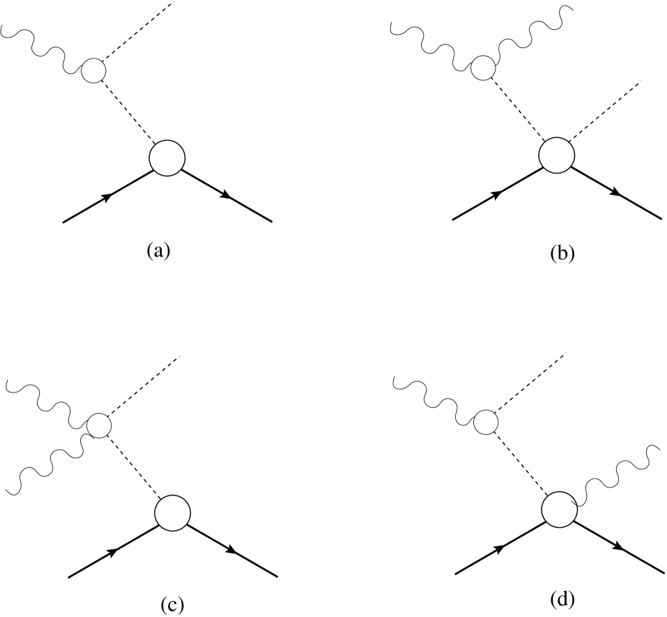
Figure 7: Pion poles in the amplitudes for electro-production (a) and associated DVCS (b, c, d).

Using Eq.(61) it is straightforward to compute the relevant commutators. From the definitions (11, 33) one gets :

$$[Q_{5}^{\alpha},j^{\mu}] = i\varepsilon_{\alpha 3\beta}j^{\mu\beta}_{5},$$ (62)

$$\,[Q_{5}^{\alpha},\sum_{f}{\cal Q}_{f}^{2}S_{f}] = \frac{i}{3}\varepsilon_{\alpha 3\beta}S^{5}_{V\alpha},$$ (63)

$$\,[Q_{5}^{\alpha},\sum_{f}{\cal Q}_{f}^{2}S^{5}_{f}] = \frac{i}{3}\varepsilon_{\alpha 3\beta}S_{V\alpha},$$ (64)

where $S^{(5)}_{V\alpha}$ are the iso-vector twist-2 operators introduced in (32,33).

V.3 Soft pion theorem for the pion electroproduction

From Eqs. (58,62) we get the soft pion theorem, which we write directly for a moving pion :

$$<N(p^{\prime})\pi^{\alpha}(k_{\pi})|j^{\mu}|N(p)>=T_{B}+\frac{1}{f_{\pi}}\varepsilon_{\alpha 3\beta}<N(p^{\prime})|j^{\mu\beta}_{5}|N(p)>+O(k_{\pi}),$$ (65)

where the Born term is obtained from Eq.(59) with :

$$\Gamma([K^{\prime}],[K]) = \left(F_{1}^{p}([t])\frac{1+\tau_{3}^{N}}{2}+F_{1}^{n}([t])\frac{1-\tau_{3}^{N}}{2}\right)\gamma^{\mu}$$ (66)

$$+ i\left(F_{2}^{p}([t])\frac{1+\tau_{3}^{N}}{2}+F_{2}^{n}([t])\frac{1-\tau_{3}^{N}}{2}\right)\frac{\sigma^{\mu\nu}([K^{\prime}]-[K])_{\nu}}{2M},\,\,$$

and $[t]=([K^{\prime}]-[K])^{2}.$ This is nothing but the low energy theorem originally derived by Nambu et al. Nambu62a ; Nambu62b . Using our assumption that $t$ is non zero in the soft pion limit, one can check that the amplitude (65) respects gauge invariance in the form

$$(p^{\prime}+k_{\pi}-p)_{\mu}\left(T_{B}+\frac{1}{f_{\pi}}\varepsilon_{\alpha 3\beta}<N(p^{\prime})|j^{\mu\beta}_{5}|N(p)>+O(k_{\pi})\right)=0,$$ (67)

that is the additional terms needed to have exact gauge invariance are in the $O(k_{\pi})$ corrections . The axial current matrix element which appears in Eq.(65) is given by Eq.(53) and involves the form factors $g_{A}(t)$ and $h_{A}(t)$. The latter is not so well known experimentally but this does not matter because it is multiplied by $p^{\prime}-p=k_{\gamma}-k_{\pi}$ where $k_{\gamma}=q-q^{\prime}$ is the photon exchanged in the BH process. In the Lorentz gauge the term proportional to $k_{\gamma}$ does not contribute to the amplitude and, because $t$ does not vanish in the soft pion limit, the term linear in $k_{\pi}$ can be pushed in the $O(k_{\pi})$ corrections despite the pion pole in $h_{A}(t)$. The rest of the calculation is just algebraic manipulation of expressions (65,66) so we do not need to give the details. For completeness we just mention the relation between the charged and cartesian pion production amplitudes :

$$T(\pi^{\pm})=\frac{T(\pi^{1}\mp i\pi^{2})}{\sqrt{2}},\,\,\,T(\pi^{0})=T(\pi^{3}).$$ (68)

V.4 Soft pion theorem for the pion twist-2 production

The soft pion theorems for pion twist-2 production folllow from Eqs(58,63,64) :

$$<N(p^{\prime})\pi^{\alpha}(k_{\pi})|\sum_{f}{\cal Q}_{f}^{2}S_{f}(x,\tilde{n})|N(p)>=$$

$$T_{B}+\frac{1}{3f_{\pi}}\varepsilon_{\alpha 3\beta}<N(p^{\prime})|S^{5}_{V\beta}(x,\tilde{n})|N(p)>+O(k_{\pi}),$$ (69)

$$<N(p^{\prime})\pi^{\alpha}(k_{\pi})|\sum_{f}{\cal Q}_{f}^{2}S^{5}_{f}(x,\tilde{n})|N(p)>=$$

$$T^{5}_{B}+\frac{1}{3f_{\pi}}\varepsilon_{\alpha 3\beta}<N(p^{\prime})|S_{V\beta}(x,\tilde{n})|N(p)>+O(k_{\pi}),$$ (70)

where the Born terms $T^{(5)}_{B}$ are obtained from Eq.(59) with the vertices $\Gamma^{(5)}$ defined by (see Eq.(56)) :

$$<N(K^{\prime})|\sum_{f}{\cal Q}_{f}^{2}S_{f}(x,\tilde{n})|N(K)> = \bar{u}(K^{\prime})\Gamma([K^{\prime}],[K],x,\tilde{n})u(K),$$ (71)

$$<N(K^{\prime})|\sum_{f}{\cal Q}_{f}^{2}S^{5}_{f}(x,\tilde{n})|N(K)> = \bar{u}(K^{\prime})\Gamma^{5}([K^{\prime}],[K],x,\tilde{n})u(K).$$ (72)

Note that we have restored the explicit dependance on $x,\tilde{n}$. Using the parametrisation (36) we have :

$$\Gamma([K^{\prime}],[K],x,\tilde{n})=\frac{2}{([K]+[K^{\prime}]).\tilde{n}}\times$$

$$\sum_{f}{\cal Q}_{f}^{2}\left(H_{f/N}([x],[\xi],[\Delta]^{2})\gamma.\tilde{n}+iE_{f/N}([x],[\xi],[\Delta]^{2})\frac{\sigma^{\mu\nu}\tilde{n}_{\mu}[\Delta]_{\nu}}{2M}\right),$$ (73)

$$\Gamma^{5}([K^{\prime}],[K],x,\tilde{n})=\frac{2}{([K]+[K^{\prime}]).\tilde{n}}\times$$

$$\sum_{f}{\cal Q}_{f}^{2}\left(\tilde{H}_{f/N}([x],[\xi],[\Delta]^{2})\gamma.\tilde{n}+\tilde{E}_{f/N}([x],[\xi],[\Delta]^{2})\frac{\tilde{n}_{.}[\Delta]}{2M}\right)\gamma^{5},$$ (74)

where the bracketed variables are, by definition (see Section IV) :

$$[x]=2\frac{x}{([K]+[K^{\prime}]).\tilde{n}},\,\,\,[\xi]=-\frac{[\Delta].\tilde{n}}{([K]+[K^{\prime}]).\tilde{n}},\,\,\,[\Delta]=[K^{\prime}]-[K].$$

From Eq.(59) we see that one has either $([K]=[p],\,[K^{\prime}]=[p^{\prime}+k_{\pi}])$ or $([K]=[p-k_{\pi}],\,[K^{\prime}]=[p^{\prime}])$. It is then apparent that the approximation $([x]\rightarrow x\,[\xi]\rightarrow\xi,\,[\Delta]\rightarrow\Delta)$ in Eqs(73,74) only induces corrections of order $k_{\pi}$. Similarly the matrix elements of $S_{V}^{(5)}$ which appear in Eqs.(69,70) can be written as :

$$<N(p^{\prime})|S_{V\alpha}(x,\tilde{n})|N(p)>=\frac{2}{(p+p^{\prime}).\tilde{n}}\times$$

$$\bar{u}(p^{\prime})\left[H_{V}(\hat{x},\hat{\xi},t)\gamma.\tilde{n}+iE_{V}(\hat{x},\hat{\xi},t)\frac{\sigma^{\mu\nu}\tilde{n}_{\mu}(p^{\prime}-p)_{\nu}}{2M}\right]\frac{\tau_{\alpha}^{N}}{2}u(p),$$ (75)

$$<N(p^{\prime})|S^{5}_{V\alpha}(\kappa,\tilde{n})|N(p)>=\frac{2}{(p+p^{\prime}).\tilde{n}}\times$$

$$\bar{u}(p^{\prime})\left[\tilde{H}_{V}(\hat{x},\hat{\xi},t)\gamma.\tilde{n}+\tilde{E}_{V}(\hat{x},\hat{\xi},t)\frac{\tilde{n}.(p^{\prime}-p)}{2M}\right]\frac{\tau_{\alpha}^{N}}{2}u(p),$$ (76)

where now the hatted variables are :

$$\hat{x}=2\frac{x}{(p+p^{\prime}).\tilde{n}},\,\,\,\hat{\xi}=-\frac{(p^{\prime}-p).\tilde{n}}{(p+p^{\prime}).\tilde{n}},$$

and $t=(p^{\prime}-p)^{2}.$ Again the approximation $\hat{x}\rightarrow x,\,\hat{\xi}\rightarrow\xi,\,(p^{\prime}-p)\rightarrow\Delta$ induces only corrections of order $k_{\pi}$. This completes our derivation of the soft pion theorem for twist-2 production.

A few comments are in order. First we see that, as promised in the introduction, the soft pion theorem for twist-2 production involves no new quantities with respect to the elastic case. Second we note that the commutator term, which involves only the isovector operators $S_{V}^{(5)}$, depends essentially on the valence quarks while the Born term, which sums over all favours, is sensitive both to the valence and the sea quarks. Third we recall that gauge invariance is not an issue for the pion twist-2 production. The couplings to the photon fields have been factorized from the beginning, see Eq.(29), independently of the final hadronic state. As in the elastic case, gauge invariance can be restored by a term which is explicitely of higher order in $t/Q$ , and thus does not contribute in the Bjorken limit Vdh99 .

VI Estimate of the $\Delta(1232)$ contribution

The soft pion theorem proposed in the previous section can be valid only for small values of the pion momentum. One can expect strong deviations when the mass of the pion-nucleon system approaches the first nucleon excitation, that is the $\Delta(1232).$ So to improve the range of validity of our estimates we now calculate the contribution of this resonance.

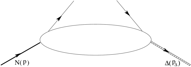
Figure 8: Delta excitation by the twist-2 operator.

As a starting point, we consider the matrix element as shown in Fig. 8, where the $\Delta$-resonance is on its mass-shell. Subsequently, we discuss the modification due to the $\Delta\rightarrow\pi N$ strong decay.

The $N\rightarrow\Delta$ matrix element for the vector twist-2 operator has the following parametrization Fra00 ; GPV01  :

$$<\Delta(p_{\Delta})|\sum_{f}{\cal Q}_{f}^{2}S_{f}(x,\,\tilde{n})|N(p)>$$ (77)

$$= {1\over 6}\;\bar{\psi}^{\beta}(p_{\Delta})\;T^{\dagger}_{3}\;\left\{\,H_{M}(x,\xi,\Delta^{2})\;\left(-{\mathcal{K}}_{\beta\kappa}^{M}\right)\,\tilde{n}^{\kappa}\right.\;+\;H_{E}(x,\xi,\Delta^{2})\;\left(-{\mathcal{K}}_{\beta\kappa}^{E}\right)\,\tilde{n}^{\kappa}$$

$$\hskip 71.13188pt\left.+\;H_{C}(x,\xi,\Delta^{2})\;\left(-{\mathcal{K}}_{\beta\kappa}^{C}\right)\,\tilde{n}^{\kappa}\right\}\,u(p),$$

where $\psi^{\beta}(p_{\Delta})$ is the Rarita-Schwinger spinor for the $\Delta$-field and $T^{\dagger}_{3}$ is the isospin $1/2\rightarrow 3/2$ transition operator, satisfying :

$$\langle\frac{3}{2}T_{z}\;|\;T^{\dagger}_{\lambda}\;|\;\frac{1}{2}t_{z}\rangle\;=\;\langle\frac{1}{2}t_{z}\;,\;1\lambda\;|\;\frac{3}{2}T_{z}\rangle\,,$$ (78)

with $t_{z}$ ($T_{z}$) the isospin projections of $N$ ($\Delta$) respectively, and where $\lambda=0,\pm 1$ indicate the spherical components of the isovector operator $T^{\dagger}$. The factor 1/6 in Eq. (77) results from the quadratic quark charge combination $(e_{u}^{2}-e_{d}^{2})/2$. Furthermore, in Eq. (77), the covariants ${\mathcal{K}}^{M,E,C}_{\beta\mu}$ are the magnetic dipole, electric quadrupole, and Coulomb quadrupole covariants Jon73  :

$${\mathcal{K}}_{\beta\mu}^{M} = -i\frac{3(M_{\Delta}+M)}{2M((M_{\Delta}+M)^{2}-\Delta^{2})}\varepsilon_{\beta\mu\lambda\sigma}P^{\lambda}\Delta^{\sigma}\;,$$

$${\mathcal{K}}_{\beta\mu}^{E} = -{\mathcal{K}}_{\beta\mu}^{M}-\frac{6(M_{\Delta}+M)}{MZ(\Delta^{2})}\varepsilon_{\beta\sigma\lambda\rho}P^{\lambda}\Delta^{\rho}\varepsilon^{\sigma}_{\,\,\mu\kappa\delta}P^{\kappa}\Delta^{\delta}\gamma^{5}\;,$$ (79)

$${\mathcal{K}}_{\beta\mu}^{C} = -i\frac{3(M_{\Delta}+M)}{MZ(\Delta^{2})}\Delta_{\beta}(\Delta^{2}P_{\mu}-\Delta\cdot P\Delta_{\mu})\gamma^{5}\;,$$

where we introduced the notation :

$$Z(\Delta^{2})=[(M_{\Delta}+M)^{2}-\Delta^{2}][(M_{\Delta}-M)^{2}-\Delta^{2}].$$ (80)

Here $P=(p_{\Delta}+p)/2$, $\Delta=p_{\Delta}-p$, and $p_{\Delta}^{2}=M_{\Delta}^{2}$ ($M_{\Delta}$ = 1232 MeV). As we are considering the production of a $\Delta$ here, we explicitely adopt the notation $\Delta^{2}$ in all expressions in this section to denote the momentum transfer squared to the hadronic system, in order not to confuse with the variable $t$ introduced before. In Eq. (77), the GPDs $H_{M}$, $H_{E}$, and $H_{C}$ for the $N\rightarrow\Delta$ vector transition are linked with the three $N\rightarrow\Delta$ vector current transition form factors $G_{M}^{*}$, $G_{E}^{*}$, and $G_{C}^{*}$ through the sum rules :

$$\int_{-1}^{1}dx\,\,H_{M,E,C}(x,\xi,\Delta^{2})=2\,\,G_{M,E,C}^{*}(\Delta^{2})\;,$$ (81)

where $G_{M,E,C}^{*}(\Delta^{2})$ are the standard magnetic dipole, electric quadrupole and Couloub quadrupole transition form factors respectively Jon73 . As is well known from experiment, the $N\rightarrow\Delta$ vector transition at small and intermediate momentum transfers is largely dominated by the $N\rightarrow\Delta$ magnetic dipole excitation, parametrized by $G_{M}^{*}(\Delta^{2})$. At $\Delta^{2}=0$, its value extracted from pion photoproduction experiments is given by $G_{M}^{*}(0)\simeq 3.02$ Tia00 . For its $\Delta^{2}$-dependence, we use a recent phenomenological parametrization Tia00 from a fit to pion electroproduction data. Given the smallness of the electric and Coulomb quadrupole $N\rightarrow\Delta$ transitions, we will neglect in the following the contribution of the GPDs $H_{E}$ and $H_{C}$.

The $N\rightarrow\Delta$ matrix element for the axial twist-2 operator has the following parametrization Fra00 ; GPV01  :

$$<\Delta(p_{\Delta})|\sum_{f}{\cal Q}_{f}^{2}S_{f}^{5}(x,\,\tilde{n})|N(p)>$$ (82)

$$= {1\over 6}\;\bar{\psi}^{\beta}(p_{\Delta})\;T^{\dagger}_{3}\;\sqrt{3\over 2}\,\left\{C_{1}(x,\xi,\Delta^{2})\,\tilde{n}_{\beta}\,+\,C_{2}(x,\xi,\Delta^{2})\,\Delta_{\beta}\,{{\Delta\cdot\tilde{n}}\over{M^{2}}}\right.$$

$$\hskip 85.35826pt+\,C_{3}(x,\xi,\Delta^{2})\,{1\over{M}}\left({\gamma.\Delta\,\tilde{n}_{\beta}-{\gamma.\tilde{n}}\,\Delta_{\beta}}\right)$$

$$\hskip 85.35826pt\left.+\,C_{4}(x,\xi,\Delta^{2})\,{2\over{M^{2}}}\left({\Delta\cdot P}\,\tilde{n}_{\beta}-\Delta_{\beta}\right)\right\}u(p)\;.$$

The GPDs $C_{1},C_{2},C_{3}$ and $C_{4}$ entering in Eq. (82) are linked with the four $N\rightarrow\Delta$ axial-vector current transition form factors $C_{5}^{A}(\Delta^{2})$, $C_{6}^{A}(\Delta^{2})$, $C_{3}^{A}(\Delta^{2})$ and $C_{4}^{A}(\Delta^{2})$, introduced by Adler Adl75 through the sum rules  :

$$\int_{-1}^{1}dx\,C_{1}(x,\xi,\Delta^{2})\, = \,2\,\,C_{5}^{A}(\Delta^{2})\,,$$

$$\int_{-1}^{1}dx\,C_{2}(x,\xi,\Delta^{2})\, = \,2\,\,C_{6}^{A}(\Delta^{2})\,,$$

$$\int_{-1}^{1}dx\,C_{3}(x,\xi,\Delta^{2})\, = \,2\,\,C_{3}^{A}(\Delta^{2})\,,$$

$$\int_{-1}^{1}dx\,C_{4}(x,\xi,\Delta^{2})\, = \,2\,\,C_{4}^{A}(\Delta^{2})\,.$$ (83)

For small momentum transfers $\Delta^{2}$, PCAC leads to a dominance of the form factors $C_{5}^{A}$ and $C_{6}^{A}$. For $C_{5}^{A}$, a Goldberger-Treiman relation for the $N\rightarrow\Delta$ transition leads to :

$$\sqrt{3\over 2}\,C_{5}^{A}(0)\,=\,\frac{f_{\pi N\Delta}}{2f_{\pi NN}}\,g_{A}\,.$$ (84)

Using the phenomenological values $f_{\pi N\Delta}\simeq 1.95$, $f_{\pi NN}\simeq 1.00$, and $g_{A}\simeq 1.267$ one obtains $C_{5}^{A}(0)\simeq 1.01$. The form factor $C_{6}^{A}(\Delta^{2})$ at small values of $\Delta^{2}$ is dominated by the pion-pole contribution, given by :

$$C_{6}^{A}(\Delta^{2})\,=\,\frac{M^{2}}{m_{\pi}^{2}-\Delta^{2}}\,C_{5}^{A}(0)\,.$$ (85)

Because we are only interested in the limit $-t,-t_{\gamma}>>m_{\pi}^{2}$, we neglect the pion pole contribution of $C_{6}$ in the following, consistent with the discussion of Section V.2.
For the two remaining Adler form factors $C_{3}^{A}$ and $C_{4}^{A}$, a detailed comparison with experimental data for $\nu$-induced $\Delta^{++}$ production led to the values Kit90  : $C_{3}^{A}(0)\simeq 0.0$ and $C_{4}^{A}(0)\simeq-0.3$. Given the smallness of these values, we will neglect in the following the contributions from the GPDs $C_{3}$ and $C_{4}$.

To provide numerical estimates for the $N\rightarrow\Delta$ DVCS amplitudes, we need a model for the three remaining ’large’ GPDs which appear in Eqs. (77,82) i.e. $H_{M}$, $C_{1}$ and $C_{2}$. Here we will be guided by the large $N_{c}$ relations discussed in Fra00 ; GPV01 . These relations connect the $N\rightarrow\Delta$ GPDs $H_{M}$, $C_{1}$, and $C_{2}$ to the $N\rightarrow N$ isovector GPDs $E^{u}-E^{d}$, $\tilde{H}^{u}-\tilde{H}^{d}$, and $\tilde{E}^{u}-\tilde{E}^{d}$ respectively. These relations are given by  :

$$H_{M}(x,\xi,\Delta^{2}) = \frac{2}{\sqrt{3}}\left[E^{u}(x,\xi,\Delta^{2})-E^{d}(x,\xi,\Delta^{2})\right]\;,$$

$$C_{1}(x,\xi,\Delta^{2}) = \sqrt{3}\left[\tilde{H}^{u}(x,\xi,\Delta^{2})-\tilde{H}^{d}(x,\xi,\Delta^{2})\right]\,,$$

$$C_{2}(x,\xi,\Delta^{2}) = \frac{\sqrt{3}}{4}\left[\tilde{E}^{u}(x,\xi,\Delta^{2})-\tilde{E}^{d}(x,\xi,\Delta^{2})\right]\,.$$ (86)

To give an idea of the accuracy of these relations, we calculate the first moment of both sides of Eq. (86) and compares their values at $\Delta^{2}=0$. For $H_{M}$, we obtain for the lhs the phenomenological value $2G_{M}^{*}(0)\simeq 6.04$, in comparison with the large $N_{c}$ prediction of $(2/\sqrt{3})\kappa^{V}\simeq 4.27$, accurate at the 30 % level .

For $C_{1}$, the phenomenological value yields $2C_{5}(0)\simeq 2.02$, whereas the large $N_{c}$ prediction yields $\sqrt{3}g_{A}\simeq 2.19$, accurate at the 10% level. For the pion-pole contribution to $C_{6}$, we obtain the same accuracy as for $C_{5}$. Furthermore, for the $N\rightarrow\Delta$ DVCS in the near forward direction, unlike the $N\rightarrow N$ DVCS case, the axial transition (proportional to the GPDs $C_{1}$ ) is numerically more important than the vector transition (parametrized by $H_{M}$). This is because $H_{M}$ is accompanied by a momentum transfer $\Delta$ in the tensor ${\mathcal{K}}^{M}$ as is seen from Eq. (79), in contrast with the structure associated with the GPD $C_{1}$. From these considerations, we estimate that the large $N_{c}$ relations of Eq. (86) for the $N\rightarrow\Delta$ transition allow us to estimate at the $\gamma^{*}p\rightarrow\gamma\Delta$ DVCS process, at the 30 % accuracy level or better.

In order to calculate the coherent sum of the non-resonant ADVCS process discussed before and the $\Delta$-resonant process, we next discuss the modification of the $\gamma^{*}N\rightarrow\gamma\Delta$ matrix elements due to the $\Delta\rightarrow\pi N$ strong decay.

The matrix element of the vector operator for the $\gamma^{*}N\rightarrow\gamma\Delta$ transition followed by $\Delta\rightarrow\pi N$ decay, is modified from Eq. (77) to :

$$<\pi N|\sum_{f}{\cal Q}_{f}^{2}S_{f}(x,\,\tilde{n})|N>_{Delta}$$ (87)

$$= -\;{{\mathcal{I}}}\frac{f_{\pi N\Delta}}{m_{\pi}}\,{k_{\pi}}^{\alpha}\,\bar{u}(p^{\prime})\frac{i\left(\gamma.p_{\Delta}+W\right)}{W^{2}-M_{\Delta}^{2}+iW\Gamma_{\Delta}(W)}$$

$$\times \left[g_{\alpha\beta}-\frac{1}{3}\gamma_{\alpha}\gamma_{\beta}-\frac{1}{3W}\left(\gamma_{\alpha}(p_{\Delta})_{\beta}-\gamma_{\beta}(p_{\Delta})_{\alpha}\right)-\frac{2}{3W^{2}}(p_{\Delta})_{\alpha}(p_{\Delta})_{\beta}\right]$$

$$\times \,{1\over 6}\,\left\{\,H_{M}(x,\xi,\Delta^{2})\;\left(-{\mathcal{K}}^{M}\right)^{\beta\kappa}\,\tilde{n}_{\kappa}\;+\;...\right\}\,u(p),$$

where $p_{\Delta}\equiv p^{\prime}+k_{\pi}$, $\Delta\equiv p^{\prime}+k_{\pi}-p$, and where we only indicated the leading transition, proportional to $H_{M}$. The isospin factor ${\mathcal{I}}$ takes on the values : ${\mathcal{I}}=2/3$ for the $\pi^{0}p$ final state, and ${\mathcal{I}}=-\sqrt{2}/3$ for the $\pi^{+}n$ final state. In the $\Delta$ propagator in Eq. (87), the energy-dependent width $\Gamma_{\Delta}(W)$ is given by :

$$\Gamma_{\Delta}(W)\,=\,\Gamma_{\Delta}(M_{\Delta})\;\cdot\;\frac{\left|\vec{k}^{*}_{\pi}(W)\right|^{3}}{\left|\vec{k}^{*}_{\pi}(M_{\Delta})\right|^{3}}\;\cdot\;\frac{M_{\Delta}}{W}\,,$$ (88)

with $\Gamma_{\Delta}(M_{\Delta})\simeq 0.120$ GeV, and where $|\vec{k}_{\pi}^{*}(W)|$ is given in Eq. (18).
Analogously, the matrix element of the axial-vector operator for the $\gamma^{*}N\rightarrow\gamma\Delta$ transition followed by $\Delta\rightarrow\pi N$ decay, is modified from Eq. (82) to :

$$<\pi N|\sum_{f}{\cal Q}_{f}^{2}S_{f}^{5}(x,\,\tilde{n})|N>_{Delta}$$ (89)

$$= -\;{{\mathcal{I}}}\frac{f_{\pi N\Delta}}{m_{\pi}}\,{k_{\pi}}^{\alpha}\,\bar{u}(p^{\prime})\frac{i\left(\gamma.p_{\Delta}+W\right)}{W^{2}-M_{\Delta}^{2}+iW\Gamma_{\Delta}(W)}$$

$$\times \left[g_{\alpha\beta}-\frac{1}{3}\gamma_{\alpha}\gamma_{\beta}-\frac{1}{3W}\left(\gamma_{\alpha}(p_{\Delta})_{\beta}-\gamma_{\beta}(p_{\Delta})_{\alpha}\right)-\frac{2}{3W^{2}}(p_{\Delta})_{\alpha}(p_{\Delta})_{\beta}\right]$$

$$\times \,{1\over 6}\,\sqrt{3\over 2}\;\left\{\,C_{1}(x,\xi,\Delta^{2})\,\tilde{n}^{\beta}\;+\;...\right\}\,u(p),$$

where we again only indicated the leading transition proportional to the GPD $C_{1}$.

Finally, in order to calculate the $\gamma^{*}p\rightarrow\gamma\pi N$ process, we also need to specify the BH process of Eq. (7) associated with the $N\rightarrow\Delta$ transition. The corresponding $\Delta$ contribution to the matrix element $J_{\nu}$ entering in Eq. (7) is given by :

$$<\pi N|j^{\nu}(0)|N>_{Delta}$$ (90)

$$= -\;{{\mathcal{I}}}\frac{f_{\pi N\Delta}}{m_{\pi}}\,{k_{\pi}}^{\alpha}\,\bar{u}(p^{\prime})\frac{i\left(\gamma\cdot p_{\Delta}+W\right)}{W^{2}-M_{\Delta}^{2}+iW\Gamma_{\Delta}(W)}$$

$$\times \left[g_{\alpha\beta}-\frac{1}{3}\gamma_{\alpha}\gamma_{\beta}-\frac{1}{3W}\left(\gamma_{\alpha}(p_{\Delta})_{\beta}-\gamma_{\beta}(p_{\Delta})_{\alpha}\right)-\frac{2}{3W^{2}}(p_{\Delta})_{\alpha}(p_{\Delta})_{\beta}\right]$$

$$\times \left\{\,G_{M}^{*}(\Delta^{2})\left(-{\mathcal{K}}^{M}\right)^{\beta\nu}+G_{E}^{*}(\Delta^{2})\left(-{\mathcal{K}}^{E}\right)^{\beta\nu}+G_{C}^{*}(\Delta^{2})\left(-{\mathcal{K}}^{C}\right)^{\beta\nu}\right\}\,u(p),$$

in terms of the same vector $N\rightarrow\Delta$ transition form factors $G_{M,E,C}^{*}$ as discussed before. The isospin factor ${\mathcal{I}}$ is the same as specified following Eq. (87).

VII Results

In the absence of available data for the $\gamma^{*}p\to\gamma\pi N$ process, we can get an idea on the accuracy of our estimates by comparing the pion production amplitudes of Eqs. (65,90), which enter in the Bethe-Heitler process, with the pion photo- and electroproduction cross sections. We are interested here in the region of not too large $-t_{\gamma}<1$ GeV², corresponding with the virtuality of the photon in the Bethe-Heitler process. In this kinematical range, a large amount of pion photo- and electroproduction data exist to compare with. In particular, the pion photoproduction cross section $\gamma p\to\pi N$ (proportional to the cross section of the associated Bethe-Heitler (ABH) process for $t_{\gamma}\to 0$), is given by

$$\left(\frac{d\sigma}{d\Omega}\right)_{c.m.}=\frac{1}{W_{\pi N}^{2}\,(8\pi)^{2}}\,\frac{|\vec{k}^{*}_{\pi}|}{E_{\gamma}^{c.m.}}\,\,\frac{1}{4}\,\sum_{\sigma}\sum_{\sigma^{\prime}}\sum_{\lambda=\pm 1}{\arrowvert\,e\,\varepsilon_{\nu}(q,\lambda)\,<\pi N|j^{\nu}(0)|N>\arrowvert}^{2},$$ (91)

where $E_{\gamma}^{c.m.}$ is the photon c.m. energy, $\varepsilon_{\nu}(q,\lambda)$ is the photon polarization vector, $W_{\pi N}$ is the $\pi N$ c.m. energy, and $j^{\nu}$ is the electromagnetic current operator. We show the results of the different model contributions discussed above to the pion photoproduction total cross sections in Fig. 9. As can be noticed from Fig. 9, our estimates consisting of a soft-pion production amplitude supplemented by a $\Delta$-resonance production mechanism reproduce the cross sections on the lower energy side of the $\Delta(1232)$ resonance. Around resonance position our simple model overestimates the cross sections by about 10 %, which is mainly due to rescattering contributions which can be included by a proper unitarization of the amplitude, which we did not perform in our simple estimate. At the higher energy side of the $\Delta(1232)$ resonance, the present model somewhat overestimates the data. Besides the unitarization, this due to the increasingly important role from the t-channel exchanges of $\rho$ and $\omega$ vector mesons in the non-resonant part of the amplitude. It is known that these vector meson exchanges yield a destructive interference on the higher energy side of the $\Delta(1232)$ resonance. Since our objective here is not to present a phenomenological model for pion photoproduction, able to precisely describe the available data, but to provide an estimate for the associated DVCS process, we do not include a proper unitarization or vector meson exchanges as one is not able at this point to model the corresponding contributions for the ADVCS process. Therefore the quality of the description shown in Fig. 9 is indicative of the quality of our corresponding estimates for the ADVCS process which are performed along the same lines, i.e. by the sum of a non-resonant soft-pion production amplitude and a $\Delta(1232)$ resonance production amplitude as outlined above.
In the following calculations we use, for the nucleon GPDs, the model described in Refs. Vdh99 ; Kiv01 ; GPV01 , to which we refer the reader for details. We construct the GPDs from a double distribution based on the forward unpolarized quark distributions of MRST01 Mar01 (for the GPD $H$) and based on the forward polarized quark distributions of Ref. Lea98 (for the GPD $\tilde{H}$). To construct the double distribution, we use a profile function with parameters $b_{val}=b_{sea}=1$ as detailed in Ref. GPV01 . For the $t$-dependence of the GPD (at the moderately small values of $t$ considered in this paper) we adopt, unless stated otherwise, a factorized ansatz by multiplying the $x$ and $\xi$ dependent function by the corresponding form factor (in $t$) so as to satisfy the first sum rule. In the calculations for the beam charge asymmetry, we also compare the results with a model for the GPDs where a D-term is added to the double distribution, with the parametrization given in Ref. Kiv01 . For all other calculations, where it is not stated explicitely, the results do not include a D-term in the model for the GPDs.

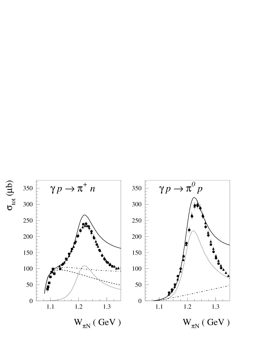
Figure 9: Total pion photoproduction cross sections for the different model contributions considered in this paper. Dashed curve : commutator contribution. Dashed-dotted curves : commutator + Born contributions. Dotted curves : $\Delta$ contribution. Solid curves : commutator + Born + $\Delta$ contributions. The data are from Ref. pitot_mcph (diamonds), Ref. pitot_macc (circles), and Ref. pitot_ahr (triangles).

In Fig. 10, we study the different ADVCS processes and show their contributions to the 7-fold differential $e^{-}p\to e^{-}\gamma\pi N$ cross sections, differential in $Q^{2},x_{B},t_{\gamma},\Phi$, the $\pi N$ invariant mass $W_{\pi N}$, and the pion solid angle $\Omega^{*}_{\pi}$ in the $\pi N$ rest frame. By comparing Figs. 9 and 10, one sees that the ratio of the non-resonant to resonant contributions is larger for the ADVCS process compared to the pion photoproduction process.

Figure 10: Different contributions to the 7-fold differential cross sections for the ADVCS processes in JLab kinematics, with pion emitted in the same direction as the recoiling $\pi N$ system (corresponding with $\theta_{\pi}^{*}=0^{o}$). Dashed-curve : commutator contribution. Dashed-dotted curves : commutator + Born contributions. Dotted curves : $\Delta$ contribution. Solid curves : commutator + Born + $\Delta$ contributions. For the $N\to\Delta$ GPDs both $C_{1}$ and $H_{M}$ are included.

In Fig. 11, we compare the 5-fold differential $e^{-}p\to e^{-}\gamma\pi N$ cross sections, i.e. integrated over the pion solid angle $\Omega^{*}_{\pi}$ , for the ABH, ADVCS and ABH + ADVCS processes for JLab kinematics. Clearly, the ABH largely dominates the cross sections. The resulting beam spin asymmetries (BSA), for a polarized lepton beam, are around 5 - 10 % for the $e^{-}p\to e^{-}\gamma\pi^{+}n$ process. For the $e^{-}p\to e^{-}\gamma\pi^{0}p$ process, the BSA grows when approaching the $\pi N$ threshold, where it reaches the same value as for the $e^{-}p\to e^{-}\gamma p$ process. This can be easily understood because at threshold, the amplitude for the $ep\to e\gamma\pi^{0}p$ process is obtained from the $ep\to e\gamma p$ process by attaching a soft pion to the initial and final proton. This is what we called the Born term in Section 5 (Fig. 5 a). This amounts to multiply the DVCS and BH amplitudes of the $ep\to e\gamma p$ process by the same factor when calculating their $ep\to e\gamma\pi^{0}p$ counterparts. Therefore, when taking the ratio of cross sections in the BSA, which is due to the interference of ABH and ADVCS, this common factor drops out and one obtains the same BSA as for the $e^{-}p\to e^{-}\gamma p$ process. Note that this is not the case for the $e^{-}p\to e^{-}\gamma\pi^{+}n$ process, where both commutator and Born terms contribute. Futhermore in the Born term for the $p\to\pi^{+}n$ transition, amplitudes involving both proton and neutron GPDs interfere according to whether the charged pion is emitted from the final or intial nucleons respectively. This results in a much smaller BSA at threshold for charged as compared to neutral pion production. When moving to higher values of $W_{\pi N}$ the $\Delta$ contribution becomes important, and the ratio of ADVCS to ABH changes compared to the $e^{-}p\to e^{-}\gamma p$ process. Around $\Delta(1232)$ resonance position, the BSA for the charged and neutral pion production channels reach comparable values, around 10 %.

Figure 11: 5-fold differential cross sections (upper panels) and corresponding beam-spin asymmetries (lower panels) for the $e^{-}p\to e^{-}\gamma\pi N$ reactions in JLab kinematics. Dotted curves : ABH; dashed curves : ADVCS; solid curves : ABH + ADVCS. The arrow gives the elastic value of the BSA for the BH + DVCS process, corresponding with $W_{\pi N}=M=0.939$ GeV.

If one does not perform a fully exclusive DVCS experiment, one actually measures the cross section

$$\frac{d\sigma^{exp}}{dQ^{2}\,dx_{B}\,dt\,d\Phi}\,=\,\frac{d\sigma(ep\to e\gamma p)}{dQ^{2}\,dx_{B}\,dt\,d\Phi}\,\left(1\,+\,R_{inel}\right),$$ (92)

with $R_{inel}$ the ratio of the integrated inelastic $ep\to e\gamma\pi N$ cross section to the cross section for the $ep\to e\gamma p$ reaction (i.e. the ‘elastic’ DVCS process), given by

$$R_{inel}\,=\,\left(\int_{M+m_{\pi}}^{W_{max}}\,dW_{\pi N}\,\frac{d\sigma(ep\to e\gamma\pi N)}{dQ^{2}\,dx_{B}\,dt\,d\Phi\,dW_{\pi N}}\right)\,/\,\frac{d\sigma(ep\to e\gamma p)}{dQ^{2}\,dx_{B}\,dt\,d\Phi}\,.$$ (93)

This is the ratio $\kappa$ introduced in Eq. (19), but written in a more familiar way. The ratio $R_{inel}$ depends upon the upper integration limit $W_{max}$, determined by the resolution of the experiment.
We can now provide an estimate of the ‘contamination’ to the BSA for a not fully exclusive experiment. In an experiment where one does not separate the $\gamma p$ and $\gamma\pi N$ final states, one actually measures

$$(BSA)^{exp}\,=\,\frac{\Delta d\sigma^{el}\,\left(1\,+\,\Delta R_{inel}\right)}{2\,d\sigma^{el}\,\left(1\,+\,R_{inel}\right)},$$ (94)

where $\Delta d\sigma^{el}$ and $d\sigma^{el}$ stand for

$$\Delta d\sigma^{el} = \frac{d\sigma_{h=+1/2}}{dQ^{2}\,dx_{B}\,dt\,d\Phi}(ep\to e\gamma p)-\frac{d\sigma_{h=-1/2}}{dQ^{2}\,dx_{B}\,dt\,d\Phi}(ep\to e\gamma p),$$

$$d\sigma^{el} = \frac{1}{2}\left(\frac{d\sigma_{h=+1/2}}{dQ^{2}\,dx_{B}\,dt\,d\Phi}(ep\to e\gamma p)+\frac{d\sigma_{h=-1/2}}{dQ^{2}\,dx_{B}\,dt\,d\Phi}(ep\to e\gamma p)\right),$$ (95)

with $h$ the lepton beam helicity. In Eq. (94), $R_{inel}$ is given as in Eq. (93), and $\Delta R_{inel}$ is the corresponding ratio of inelastic to elastic DVCS helicity cross sections :

$$\Delta R_{inel}\,=\,\left(\int_{M+m_{\pi}}^{W_{max}}\,dW_{\pi N}\,\frac{\Delta d\sigma(ep\to e\gamma\pi N)}{dQ^{2}\,dx_{B}\,dt\,d\Phi\,dW_{\pi N}}\right)\,/\,\frac{\Delta d\sigma(ep\to e\gamma p)}{dQ^{2}\,dx_{B}\,dt\,d\Phi}.$$ (96)

From Eq. (94), one sees that for a not fully exclusive experiment the ‘elastic’ beam-spin asymmetry $(BSA)^{el}$ for the $ep\to e\gamma p$ process is related to the measured beam-spin asymmetry $(BSA)^{exp}$ through :

$$(BSA)^{el}\,\equiv\,\frac{\Delta d\sigma^{el}}{2\;d\sigma^{el}}\,=\,R_{BSA}\,\cdot\,(BSA)^{exp},$$ (97)

where the correction factor $R_{BSA}$ is given by :

$$R_{BSA}\,=\,\frac{1\,+\,R_{inel}}{1\,+\,\Delta R_{inel}}.$$ (98)

In Fig. 12, we show the ratios $R_{inel}$ and $\Delta R_{inel}$. One sees that when integrating up to $W_{max}\simeq 1.35$ GeV, the helicity cross sections ratio $\Delta R_{inel}$ reaches about 10 % for $\gamma\pi^{+}n$ and $\gamma\pi^{0}p$ final states separately. On the other hand, the unpolarized cross section ratio $R_{inel}$ is much larger and reaches about 40 % for each channel separately. This difference originates in the different ratio of the ABH cross section as compared to the corresponding ADVCS ratio. This different ratio for the ABH and ADVCS processes has as consequence that the BSA, which is due to an interference of both, receives an important correction in an experiment where the final state cannot be fully resolved.

Figure 12: Ratios $R_{inel}$ and $\Delta R_{inel}$ of $e^{-}p\to e^{-}\gamma\pi N$ (ABH + ADVCS) to $e^{-}p\to e^{-}\gamma p$ (BH + DVCS) cross sections according to Eqs. (93, 96) as function of the upper integration limit $W_{max}$ in JLab kinematics. Dashed (solid) curves : ratio of unpolarized (polarized) cross sections respectively.

In Fig. 13, we show the resulting correction factor for the BSA defined in Eq. (98) for JLab kinematics. For an experiment which measures an $e^{-}$ and a proton, and which reconstructs the final $\gamma$ from the missing mass, but where the resolution does not permit to fully separate the $\gamma p$ final state from a $\gamma\pi^{0}p$ final state, such as in the bulk of the events of the first DVCS experiment at CLAS Step02 , one obtains a correction factor of around 1.3 when integrating up to $W_{max}\simeq 1.35$ GeV in the kinematics considered in Fig. 13. For an experiment which only measures an $e^{-}$ and a $\gamma$ in the final state and where the resolution does not permit to separate the $p$ hadronic final state from the $\pi^{+}n$ and $\pi^{0}p$ hadronic final states, the correction factor, integrated up to $W_{max}\simeq 1.35$ GeV, amounts to about 1.6 in the same kinematics.

Figure 13: Correction factor according to Eq. (98) to apply to the measured BSA to extract the $e^{-}p\to e^{-}\gamma p$ BSA, when the measurement is not fully exclusive. The correction factors are given for the situations where the $\gamma p$ final state is contaminated either by $\gamma\pi^{+}n$ (upper panel), by $\gamma\pi^{0}p$ (middle panel), or by both $\gamma\pi^{+}n$ and $\gamma\pi^{0}p$ (lower panel). The correction is given as function of the upper integration limit $W_{max}$ in JLab kinematics.

In Figs. 14 - 16, we study the corresponding effects in the kinematics accessible in the HERMES experiment.
One sees from Fig. 14 that in the kinematics accessible at HERMES, the ABH still dominates the cross sections. The interference of the ABH and ADVCS processes leads to a BSA which is around 10% for the $e^{-}p\to e^{-}\gamma\pi^{+}n$ reaction. For the $e^{-}p\to e^{-}\gamma\pi^{0}p$ reaction, the BSA rises towards $\pi N$ threshold where it reaches the value of the BSA for the $e^{-}p\to e^{-}\gamma p$ reaction, as discussed before. Around the $\Delta(1232)$ resonance position, the BSA for the $e^{-}p\to e^{-}\gamma\pi^{0}p$ reaction reaches about 15 %.
For the present DVCS experiments at HERMES Air02 where the experimental resolution does not allow to fully reconstruct the final state, it is important to estimate the contribution of the $\gamma\pi^{+}n$ and $\gamma\pi^{0}p$ final states, which we show in Fig. 15. When integrating the cross sections up to $W_{max}\simeq 1.35$ GeV, the helicity cross sections ratio $\Delta R_{inel}$ reaches about 3 % (5 %) for the $\gamma\pi^{+}n$ ($\gamma\pi^{0}p$) final states respectively. On the other hand, the unpolarized cross section ratio $R_{inel}$ reaches about 10 % for each channel separately. This different ratio leads to a correction for the BSA in an experiment where the final state cannot be fully resolved, which is shown in Fig. 16. For kinematics close to the first DVCS experiment at HERMES Air02 which measured an $e^{-}$ and a $\gamma$ and where the resolution did not permit to separate the $p$ hadronic final state from the $\pi^{+}n$ and $\pi^{0}p$ hadronic final states, one sees that the correction factor on the BSA due to the $\Delta$ resonance region, i.e. integrated up to $W_{max}\simeq 1.35$ GeV, amounts to about 1.1 .

Figure 14: 5-fold differential cross sections (upper panels) and corresponding beam-spin asymmetries (lower panels) for the $e^{-}p\to e^{-}\gamma\pi N$ reactions in HERMES kinematics. Dotted curves : ABH; dashed curves : ADVCS; solid curves : ABH + ADVCS. The arrow gives the elastic value of the BSA for the BH + DVCS process, corresponding with $W_{\pi N}=M=0.939$ GeV.

Figure 15: Ratio of $e^{-}p\to e^{-}\gamma\pi N$ (ABH + ADVCS) to $e^{-}p\to e^{-}\gamma p$ (BH + DVCS) cross sections according to Eqs. (93, 96) as function of the upper integration limit $W_{max}$ in HERMES kinematics. Dashed (solid) curves : ratio of unpolarized (polarized) cross sections respectively.

Figure 16: Correction factor according to Eq. (98) to apply to the measured BSA to extract the $e^{-}p\to e^{-}\gamma p$ BSA, when the measurement is not fully exclusive. The correction factors are given for the situations where the $\gamma p$ final state is contaminated either by $\gamma\pi^{+}n$ (upper panel), by $\gamma\pi^{0}p$ (middle panel), or by both $\gamma\pi^{+}n$ and $\gamma\pi^{0}p$ (lower panel). The correction is given as function of the upper integration limit $W_{max}$ for HERMES kinematics.

We next discuss the beam charge asymmetries (BCA) between the $e^{+}p\to e^{+}\gamma\pi N$ and $e^{-}p\to e^{-}\gamma\pi N$ processes. The BCA in kinematics accessible at HERMES is shown in Fig. 17 for two models of the GPDs, one including the D-term and one without the D-term contribution. As for the BSA, one sees that for the $\gamma\pi^{0}p$ final state, the BCA reaches the same value as for the elastic DVCS process when approaching the $\pi N$ threshold. Furthermore, one sees that since the D-term only contributes to the Born terms, it mainly manifests itsef in the neutral pion production channel around threshold, while its effect is very small on the charged pion production channel. Around $\Delta(1232)$ resonance, the effect of the D-term is negligible.
The BCA between the $e^{+}p\to e^{+}\gamma X$ and $e^{-}p\to e^{-}\gamma X$ processes has been measured at HERMES Ell02 . Because this experiment does not allow to distinguish the hadronic final states $X=p$ from $X=\pi^{+}n$ and $X=\pi^{0}p$, it is of interest to estimate the ‘contamination’ by the associated pion production. An experiment which does not separates $X=p$ from $X=\pi N$ measures :

$$(BCA)^{exp}\,=\,\frac{\sigma_{e^{+}}^{el}\,\left(1\,+\,R_{+}\right)\;-\;\sigma_{e^{-}}^{el}\,\left(1\,+\,R_{-}\right)}{\sigma_{e^{+}}^{el}\,\left(1\,+\,R_{+}\right)\;+\;\sigma_{e^{-}}^{el}\,\left(1\,+\,R_{-}\right)},$$ (99)

where $\sigma_{\pm}^{el}$ stands for the cross section $d\sigma(e^{\pm}p\to e^{\pm}\gamma p)/(dQ^{2}\,dx_{B}\,dt\,d\Phi)$ of the ’elastic’ process, and where the ratios $R_{\pm}$ stand for :

$$R_{\pm}\,=\,\frac{1}{\sigma_{e^{\pm}}^{el}}\;\int_{M+m_{\pi}}^{W_{max}}\,dW_{\pi N}\,\frac{d\sigma(e^{\pm}p\to e^{\pm}\gamma\pi N)}{dQ^{2}\,dx_{B}\,dt\,d\Phi\,dW_{\pi N}}.$$ (100)

From Eq. (99), one sees that for a not fully exclusive experiment the ‘elastic’ $(BCA)^{el}$ is obtained from the measured $(BCA)^{exp}$ through :

$$(BCA)^{el}\,\equiv\,\frac{\sigma_{e^{+}}^{el}\;-\;\sigma_{e^{-}}^{el}}{\sigma_{e^{+}}^{el}\;+\;\sigma_{e^{-}}^{el}}\,=\,R_{BCA}\,\cdot\,(BCA)^{exp},$$ (101)

where the correction factor $R_{BCA}$ is given by :

$$R_{BCA}\,=\,\frac{1\,+\,(\sigma_{e^{+}}^{el}R_{+}\,+\,\sigma_{e^{-}}^{el}R_{-})/(\sigma_{e^{+}}^{el}\,+\,\sigma_{e^{-}}^{el})}{1\,+\,(\sigma_{e^{+}}^{el}R_{+}\,-\,\sigma_{e^{-}}^{el}R_{-})/(\sigma_{e^{+}}^{el}\,-\,\sigma_{e^{-}}^{el})}.$$ (102)

The correction factor $R_{BCA}$ is shown in Fig. 18 for HERMES kinematics. For an experiment which does not separate the $p$ hadronic final state from the $\pi^{+}n$ and $\pi^{0}p$ hadronic final states, the correction factor on the BCA, integrated up to $W_{max}\simeq 1.35$ GeV, amounts to about 1.8 for the model without D-term and reaches around 1.1 for the model with D-term. The much smaller correction in the presence of the D-term can be understood as in this case the elastic BCA has the same sign and similar magnitude as the inelastic BCA around $\Delta(1232)$ resonance. On the other hand, in the absence of the D-term contribution, the elastic BCA is small and negative, yielding a significant different result from the positive BCA around $\Delta(1232)$ resonance. Therefore, the resulting correction factor is much larger for the GPD model without D-term. As the correction of the BCA can be sizeable according to the model for the GPDs, this clearly calls for a fully exclusive measurement to separate the different final states, in order to reliably extract information on the GPDs. Such an experiment is planned in the near future at HERMES using a recoil detector Herrec .

Figure 17: Beam charge asymmetries (BCA) for the ABH + ADVCS processes in HERMES kinematics. The result is shown for 2 different models of the GPDs : without D-term (dashed curves) and with D-term (solid curves). The corresponding arrows give the elastic value of the BCA for the BH + DVCS process, corresponding with $W_{\pi N}=M=0.939$ GeV.

Figure 18: Correction factor according to Eq. (102) to apply to the measured BCA to extract the BCA between the ‘elastic’ processes $e^{\pm}p\to e^{\pm}\gamma p$, when the measurement is not fully exclusive. The correction factors are given for the situations where the $\gamma p$ final state is contaminated either by $\gamma\pi^{+}n$ (upper panel), by $\gamma\pi^{0}p$ (middle panel), or by both $\gamma\pi^{+}n$ and $\gamma\pi^{0}p$ (lower panel). The correction is given as function of the upper integration limit $W_{max}$ for HERMES kinematics. The solid and dashed curves correspond with the two GPD models as described in Fig. 17.

In Figs. 19-22, we show the results for kinematics accessible at COMPASS Compass . Fig. 19 shows the differential cross section and BSA for the $\mu^{+}p\to\mu^{+}\gamma\pi N$ processes. In contrast to the previous results for JLab and HERMES kinematics, we see that at COMPASS the $\mu^{+}p\to\mu^{+}\gamma\pi N$ cross section is dominated by the ADVCS process. The interference with the small BH yields only a small value for the BSA. Due to the dominance of the ADVCS over the BH, one sees in Fig. 20 an opposite trend for the ratios $R_{inel}$ and $\Delta R_{inel}$ of Eqs. (93, 96) in comparison with the ones shown in Figs. 12 and 15 for JLab and HERMES respectively. The larger value of $\Delta R_{inel}$ compared to $R_{inel}$, in particular for $\mu^{+}p\to\mu^{+}\gamma\pi^{0}p$, leads to a correction factor $R_{BSA}$ of Eq. (98) which is slightly smaller than one. For an experiment which does not permit to separate the $p$ hadronic final state from the $\pi^{+}n$ and $\pi^{0}p$ hadronic final states, the correction factor on the BSA due to the $\Delta$ resonance region, i.e. integrated up to $W_{max}\simeq 1.35$ GeV, amounts to a value around 0.95 at COMPASS.
In Figs. 21, 22 we study the BCA at COMPASS. To obtain sizeable interferences with the BH process, we show the results for a lower beam energy of 100 GeV as also accessible at COMPASS. We compare the results for two models of the GPDs. The first model consists of a factorized ansatz for the $t$-dependence (compared to the $x$- and $\xi$ dependences) of the GPDs as used in the previous calculations, and does not include the D-term. The second model includes the D-term and uses an unfactorized Regge ansatz for the GPDs as specified in Ref. GPV01 . As can be seen from Fig. 21, the $\pi^{0}$ production process is mainly sensitive to the differences between those models and at the threshold the BCA for the $\mu^{\pm}p\to\mu^{\pm}\gamma\pi^{0}p$ and $\mu^{\pm}p\to\mu^{\pm}\gamma p$ reactions are the same. For an experiment which does not separate the $p$ hadronic final state from the $\pi^{+}n$ and $\pi^{0}p$ hadronic final states, we estimate the correction factors on the BCA in Fig. 22. When integrating the $\pi N$ spectrum up to $W_{max}\simeq 1.35$ GeV, the correction factor on the BCA asymmetry due to both $\pi^{0}p$ and $\pi^{+}n$ channels amounts to about 1.35 for the model without D-term and reaches around 1.05 for the model with D-term.

Figure 19: 5-fold differential cross sections (upper panels) and corresponding beam-spin asymmetries (lower panels) for the $\mu^{+}p\to\mu^{+}\gamma\pi N$ reactions in COMPASS kinematics. Dotted curves : ABH; dashed curves : ADVCS; solid curves : ABH + ADVCS. The arrow gives the elastic value of the BSA for the BH + DVCS process, corresponding with $W_{\pi N}=M=0.939$ GeV.

Figure 20: Ratio of $\mu^{+}p\to\mu^{+}\gamma\pi N$ (ABH + ADVCS) to $\mu^{+}p\to\mu^{+}\gamma p$ (BH + DVCS) cross sections according to Eqs. (93, 96) as function of the upper integration limit $W_{max}$ in COMPASS kinematics. Dashed (solid) curves : ratio of unpolarized (polarized) cross sections respectively.

Figure 21: Beam charge asymmetries (BCA) for the ABH + ADVCS processes in COMPASS kinematics. The result is shown for 2 different models of the GPDs. Dashed curve : GPD model with factorized t-dependence and without D-term. Solid curve : GPD model with unfactorized t-dependence and with D-term. The corresponding arrows give the elastic value of the BCA for the BH + DVCS process, corresponding with $W_{\pi N}=M=0.939$ GeV.

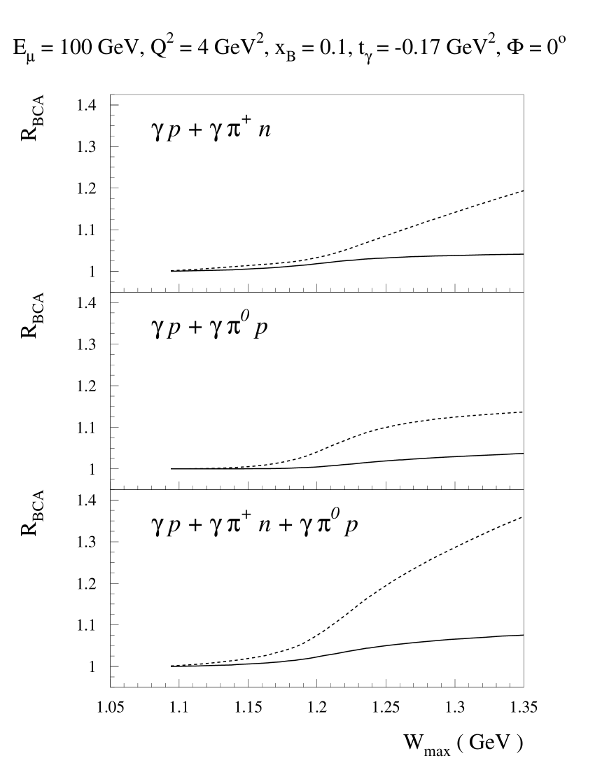
Figure 22: Correction factor according to Eq. (102) to apply to the measured BCA to extract the BCA between the ‘elastic’ processes $\mu^{\pm}p\to\mu^{\pm}\gamma p$, when the measurement is not fully exclusive. The correction factors are given for the situations where the $\gamma p$ final state is contaminated either by $\gamma\pi^{+}n$ (upper panel), by $\gamma\pi^{0}p$ (middle panel), or by both $\gamma\pi^{+}n$ and $\gamma\pi^{0}p$ (lower panel). The correction is given as function of the upper integration limit $W_{max}$ for COMPASS kinematics. The solid and dashed curves correspond with the two GPD models as described in Fig. 21.

VIII Conclusion

We have developed a model to calculate the cross section for producing an extra low energy pion in the photon electro-production reaction. Our primary goal is to provide a reasonable estimate of the contamination of the ’elastic’ process by this associated reaction when the experimental data are not fully exclusive. For the various observables which are generally considered of interest we have defined correction factors by integrating the associated reaction cross sections up to a given cutoff.

To build our model we have used the time honored soft pion technique based on current algebra and chiral symmetry. In the case of the DVCS reaction, which we always consider in the Bjorken limit, we have assumed that it was possible to first invoke the factorization theorem and then to use chiral symmetry to evaluate the matrix elements of the twist two operators involving one soft pion. Our derivation applies to the kinematical region $m_{\pi}^{2}<<-t<<Q^{2}$ of DVCS type processes, which corresponds with the kinematical range of experiments considered at JLab, HERMES and COMPASS. The order in which one applies the chiral limit ($m_{\pi}\to 0$) and the Bjorken limit ($Q^{2}\to\infty$) is a point which certainly deserves further attention, see e.g. Ref. PPS01 where new low-energy theorems were derived for the $\gamma^{*}N\to\pi N$ process at large virtualities of the photon ($Q^{2}>>\Lambda_{QCD}^{3}/m_{\pi}$). In this respect, the chiral perturbation theory approach developed in Refs. Chen01 ; Arndt02 to study the quark mass dependence of the parton distribution may be useful. For such a systematic chiral perturbation expansion to converge, one also sees that the momentum transfer $-t$ should be bound from above, and be smaller than the chiral symmetry breaking scale of order $(4\pi f_{\pi})^{2}$.

The advantage of our approach is that the GPDs necessary to calculate the associated pion production are the same as in the elastic DVCS process. So, in a relative sense, our estimate is largely independent of the details of the GPDs.

To extend our estimate to pions of higher energy we have added the P-wave production assuming it is dominated by the $\Delta(1232)$ isobar production. Here, following the approach of Ref. Fra00 we have used the large $N_{c}$ limit to relate the GPDs of the $N\rightarrow\Delta$ transition to the $N\rightarrow N$ ones. Again this minimizes the model dependence of our results.

For those experiments which do have the resolution to measure the $\gamma^{*}p\to\gamma\pi N$ process, in particular in the $\Delta(1232)$ resonance region Michel03 , our calculation provides a prediction using the large $N_{c}$ limit for the $N\rightarrow\Delta$ GPDs. The measurement of the $\gamma^{*}p\to\gamma\Delta\to\gamma\pi N$ process holds the prospect to access information on the quark distributions in the $\Delta$ resonance, which are totally unknown at present.

Generally the DVCS amplitude must be added coherently to the Bethe-Heitler amplitude. This is also true for the associated reactions and we have used the same approach to estimate the associated BH and DVCS amplitudes. For the BH amplitude this amounts to calculate the pion electro-production amplitude and this gives us a chance to rate the validity of our results by comparing to the existing data. We find that, for the integrated cross sections, our estimate are probably valid up to $W_{max}=1.35\leavevmode\nobreak\ {\rm GeV}$.

We have performed our calculations for a set of kinematical conditions which are representative of the present or planned experiments at JLab, HERMES and COMPASS. In a regime where the ADVCS process dominates the cross section, such as is the case at COMPASS, we find that the pionic contamination (integrated up to $W_{max}=1.35\leavevmode\nobreak\ {\rm GeV}$) never exceeds 10%. In a kinematical regime where the ABH process dominates, such as is typically the case at HERMES and in particular at JLab, the pionic contamination may become much larger and calls for fully exclusive experiments. In particular, it has an effect on the beam spin and beam charge asymmetries. For instance the correction to the BSA due to charged (neutral) pions in JLab kinematics can reach 30% each for an experiment which is not able to distinguish a $N$ from a $\pi N$ for a cutoff $W_{max}=1.35\leavevmode\nobreak\ {\rm GeV}$. The effect on the BSA due to the $\pi^{0}p$ and $\pi^{+}n$ production in HERMES kinematics is of the order of 10%. On the other hand the correction factor on the BCA to obtain the ‘elastic’ BCA from an experiment not able to distinguish a $N$ from a $\pi N$ can be as large as a factor 1.8 at HERMES and 1.35 at COMPASS depending on the model for the GPDs.

To summarize, for a cutoff of $W_{max}=1.35\leavevmode\nobreak\ {\rm GeV}$ the correction to the cross sections is moderate but for the BSA and BCA our calculations indicate that it is wise to consider fully exclusive experiments.

References

• (1) X. Ji, Phys. Rev. Lett. 78, 610 (1997); Phys. Rev. D 55, 7114 (1997).
• (2) A.V. Radyushkin, Phys. Lett. B 380, 417 (1996).
• (3) X. Ji, and J. Osborne, Phys. Rev. D 58, 094018 (1998).
• (4) A.V. Radyushkin, Phys. Rev. D 58, 114008 (1998).
• (5) J.C. Collins, and A. Freund, Phys. Rev. D 59, 074009 (1999).
• (6) A. Airapetian et al. (HERMES Collaboration), Phys. Rev. Lett. 87, 182001 (2001).
• (7) S. Stepanyan et al. (CLAS Collaboration), Phys. Rev. Lett. 87, 182002 (2001).
• (8) P.Y. Bertin, C.E. Hyde-Wright, and F. Sabatié, spokespersons JLab (Hall A) experiment E-00-110.
• (9) N. d’Hose, E. Burtin, P.A.M. Guichon, S. Kerhoas-Cavata, J. Marroncle and L. Mossé, Nucl. Phys. A 711, 160c (2002).
• (10) L. Favart, Nucl. Phys. A 711, 165c (2002).
• (11) M. Guidal et al., hep-ph/0304252.
• (12) L.L. Frankfurt, M. V. Polyakov, M. Strikman, and M. Vanderhaeghen, Phys. Rev. Lett. 84, 2589 (2000).
• (13) X. Ji, W. Melnitchouk, and X. Song, Phys. Rev. D 56, 1(1997).
• (14) M. Vanderhaeghen, P.A.M. Guichon, and M. Guidal, Phys. Rev. D 60, 094017 (1999).
• (15) X. Ji, J. Phys. G 24, 1181 (1998).
• (16) P.A.M. Guichon, and M. Vanderhaeghen, Prog. Part. Nucl. Phys. 41, 125 (1998).
• (17) A.V. Radyushkin, hep-ph/0101225.
• (18) K. Goeke, M.V. Polyakov and M. Vanderhaeghen, Prog. Part. Nucl. Phys. 47, 401 (2001).
• (19) V. de Alfaro, S. Fubini, G. Furlan and C. Rossetti, Nuovo Cimento 62A, 497 (1968).
• (20) G. Furlan, N. Paver and C. Verzegnassi, Springer Tracts in Modern Physics 62, 118 (1972).
• (21) S. Adler, R. Dashen, “Current algebras", Benjamin, NewYork, 1968.
• (22) R.F. Dashen and M. Weinstein, Phys.Rev. 183, 1261 (1967).
• (23) P. Langacker and H. Pagels, Phys. Rev. D8, 4595 (1973).
• (24) Y. Nambu and D. Luriè, Phys. Rev.125, 1429 (1962).
• (25) Y. Nambu and E. Shrauner, Phys. Rev. 128, 862 (1962).
• (26) H.F. Jones, M.D. Scadron, Ann. of Phys. 81, 1 (1973).
• (27) L. Tiator, D. Drechsel, O. Hanstein, S.S. Kamalov, and S.N. Yang, Nucl. Phys. A689, 205 (2001).
• (28) S. Adler, Ann. Phys. (N.Y.) 50, 189 (1968); Phys. Rev. D 12, 2644 (1975).
• (29) T. Kitagaki et al, Phys. Rev. D 42, 1331 (1990).
• (30) D. A. McPherson et al. Phys. Rev. 136, B1465 (1964).
• (31) M. MacCormick et al., Phys. Rev. C 53, 41 (1996).
• (32) J. Ahrens et al., Phys. Rev. Lett. 84, 5950 (2000).
• (33) N. Kivel, M.V. Polyakov, and M. Vanderhaeghen, Phys. Rev. D 63, 114014 (2001).
• (34) A.D. Martin, R.G. Roberts, W.J. Stirling, R.S. Thorne, Eur. Phys. J. C 23, 73 (2002).
• (35) E. Leader, A.V. Sidorov and D.B. Stamenov, Phys. Rev. D 58, 114028 (1998).
• (36) F. Ellinghaus (on behalf of the HERMES Collaboration), hep-ex/0207029.
• (37) HERMES Recoil group, Technical Design Report, DESY PRC 01-01, 2002.
• (38) P.V. Pobylitsa, M.V. Polyakov, and M. Strikman, Phys. Rev. Lett. 87, 022001 (2001).
• (39) J.-W. Chen and X. Ji, Phys. Rev. Lett. 87, 152002 (2001).
• (40) D. Arndt and M.J. Savage, Nucl. Phys. A697, 429 (2002).