Electric charge and magnetic moment of massive neutrino

Abstract

We consider the massive Dirac neutrino electric charge and magnetic moment within the context of the standard model supplied with $\mathrm{SU}(2)$-singlet right-handed neutrino in arbitrary $R_{\xi}$ gauge. Using the dimensional-regularization scheme we start with the calculations of the one-loop contributions to the neutrino electromagnetic vertex function exactly accounting for the neutrino mass. We examine the decomposition of the massive neutrino electromagnetic vertex function. It is found by means of direct calculations that the massive neutrino vertex function contains only the four form factors. Then we derive the closed integral expressions for different contributions to the neutrino electric form factor, electric charge, and magnetic moment. For several one-loop contributions to the neutrino charge and magnetic moment, that were calculated previously with mistakes by the other authors, we find the correct results. We show that the electric charge for the massive neutrino is a gauge independent and vanishing parameter in the first two orders of the expansion over the neutrino mass parameter $b=(m_{\nu}/M_{W})^{2}$. From the obtained closed two-integral expression for a massive neutrino electric form factor it is also possible to derive the neutrino charge radius. In the particular choice of the ’t Hooft-Feynman gauge we also demonstrate that the neutrino charge is zero in all orders of expansion over $b$, i.e. for arbitrary mass of neutrino. For each of the diagrams contributing to the neutrino magnetic moment, we obtain the expressions accounting for the leading (zeroth) and next-to-leading (first) order in $b$, where the gauge dependence is shown explicitly. Each of the contributions is finite and the sum of all contributions turns out to be gauge-independent. Our calculations also enable us to obtain the neutrino magnetic moment in theoretical models that differ from each other by the values of particles’ masses, including the case of a very heavy neutrino. The general expression for the massive neutrino magnetic form factor is presented.

I Introduction

The recent experimental studies of the astrophysical and terrestrial neutrino fluxes provide the convincing evidences for the non-vanishing neutrino mass and neutrino mixing Bilenky et al. (2003). These properties of neutrino are attributes of the physics beyond a scope of the standard model. An important information on the structure of the future model of interaction can be obtained in the investigation of radiative corrections to the properties of neutrino that in principle can be also verified in experiments. A critical test of a theoretical model is provided by the direct calculation of such characteristics of neutrino as its electric charge and magnetic moment. In this respect it is interesting to examine the gauge and neutrino mass dependence of these quantities.

The electric charge and magnetic moment are the most important static electromagnetic properties of a particle. Their values are determined by corresponding form factors if the external photon is on a mass shell. In spite of the fact that the electromagnetic form factors are not measurable properties of a particle at nonzero momentum transfer, there are processes where the off-shell external photons are important. The example is the radiative corrections to the fermion-fermion scattering. The fermion electromagnetic vertex function and, in particular, its representation in terms of form factors in the case of off-shell external photon has been considered in Refs. Kim (1976); Bég et al. (1978) within various gauge theories.

To the best of our knowledge, however, there is no direct one-loop calculations of the neutrino electromagnetic vertex as well as of the neutrino charge and magnetic moment which are performed within the context of the standard model in the renormalizable $R_{\xi}$ gauge and which explicitly take into account the neutrino mass. It is worth to be noted here that the massive Majorana neutrino cannot have neither magnetic nor electric dipole moment. Due to the lepton flavour non-conservation that has been confirmed in the neutrino experiments, a neutrino could have flavour-off-diagonal transition magnetic moment, which is also allowable for Majorana neutrino. The differences between the Dirac and Majorana electromagnetic properties are explained in detail in Kayser (1982).

The neutrino vertex function in the limit of small neutrino mass was considered in Ref. Lee and Shrock (1977). There are several works where the neutrino charge is calculated within the standard model using the unitary, linear $R_{\xi}$, and ’t Hooft-Feynman gauges Bardeen et al. (1972); Marciano and Sirlin (1980); Sakakibara (1981); Lucio Martínez et al. (1984). The one-loop contributions to the neutrino magnetic moment in the standard model have been also considered previously Lee and Shrock (1977); Fujikawa and Shrock (1980); Shrock (1982); Egorov et al. (1999). The vanishing of the massless neutrino charge emerges from the unbroken electromagnetic gauge invariance. The corresponding Ward identity has been derived in Refs. Denner et al. (1995); Cabral-Rosetti et al. (2000) using the background field method. In the recent studies Cabral-Rosetti et al. (2000) a computation of one-loop electroweak diagrams, which contribute to the neutrino charge and magnetic moment in the background field method and in the linear $R_{\xi}$ gauge, is presented. However, all the previous calculations of the neutrino charge have been performed under assumption of a vanishing neutrino mass. With respect to the neutrino magnetic moment, an according treatment of this quantity was also performed to the leading order in the neutrino mass that is valid for the case of neutrino being much lighter than the corresponding charged lepton, $m_{\nu_{\ell}}\ll m_{\ell}$. In addition, the results presented in Ref. Cabral-Rosetti et al. (2000) for the gauge-fixing parameter dependence of several one-loop contributions to the neutrino charge and magnetic moment are incorrect.

In this paper we consider the massive Dirac neutrino charge and magnetic form factors in the context of the standard model supplied with $\mathrm{SU}(2)$-singlet right-handed neutrino. Using the dimensional-regularization scheme, we start (Section II) with the calculations of the one-loop Feynman diagrams that contribute to the neutrino electromagnetic vertex function $\Lambda_{\mu}(q)$ in the general $R_{\xi}$ gauge. It should be noted that, contrary to the previous studies, we explicitly account for non-vanishing neutrino mass. In Section II.1 we examine the structure of the massive neutrino electromagnetic vertex function. The decomposition of a fermion vertex function in terms of the four well-known electromagnetic form factors (presented, for instance, in Refs. Kim (1976); Bég et al. (1978)) has been established using general principles such as the Lorentz and CP invariance and the hermicity. We analyze this decomposition and verify it by means of direct calculations in the case of massive neutrino within the standard model supplied with $\mathrm{SU}(2)$-singlet right-handed neutrino. Such direct calculations were never undertaken previously.

We present the general expressions for the contributions to neutrino electric form factor in Section III. Then in Section III.1 we study the neutrino electric charge and analyze neutrino mass and gauge dependence of corresponding contributions arising from different Feynman diagrams. Although there is no doubt that the neutrino electric charge within the standard model is a gauge independent and vanishing quantity, however this fact has not been yet actually demonstrated in the case of a massive neutrino. Our calculations allow us to determine the neutrino mass and gauge parameter dependence of the one-loop contributions to the neutrino charge. We also obtain a correct gauge dependence for the contributions of several diagrams to the neutrino charge that have been calculated in Ref. Cabral-Rosetti et al. (2000) with mistakes. Within the one-loop level we show that the neutrino electric charge is gauge independent and vanishing in the ”zeroth” and first order of the expansion over the neutrino mass parameter $b=\left(m_{\nu}/M_{W}\right)^{2}$. Moreover, for the particular choice of the ’t Hooft-Feynman gauge we also demonstrate that the neutrino charge is zero for arbitrary neutrino mass, i.e. in all orders of the expansion over the parameter $b$. The obtained formulae can be used for studying the massive neutrino charge radius (Section III.3).

In Section IV we consider the neutrino magnetic form factor using the one-loop contributions to the neutrino electromagnetic vertex derived in Section II. For each of the contributions to the neutrino magnetic moment we derive the integral representations that exactly account for the gauge-fixing parameters as well as for the neutrino mass and corresponding charged lepton mass parameters ($b$ and $a=\left(m_{\ell}/M_{W}\right)^{2}$). Then for each of the diagrams we perform an integration and obtain the explicitly gauge-dependent contributions to the neutrino magnetic moment accounting for the leading (zeroth) and next-to-leading (first) order in the expansion over neutrino mass parameter $b$. The sum of all the contributions turns out to be gauge parameter independent. However, our results for several contributions to the neutrino magnetic moment in the leading order in the neutrino mass disagree with those of Ref. Cabral-Rosetti et al. (2000) for the corresponding contributions. In particular, contrary to the results of Ref. Cabral-Rosetti et al. (2000), not all the contributions are gauge independent. Our calculations enable one to reproduce the correct value for the neutrino magnetic moment in any gauge including also the unitary gauge for which the results of Ref. Cabral-Rosetti et al. (2000) are incorrect. In this Section we get final expressions for the massive neutrino magnetic moment in the various ranges of neutrino, charged lepton and $W$ boson masses: $m_{\nu}\ll m_{\ell}\ll M_{W}$, $m_{\ell}\ll m_{\nu}\ll M_{W}$, and $m_{\ell}\ll M_{W}\ll m_{\nu}$. The last case amounts to a very heavy neutrino that is not excluded by the LEP data (see, e.g., Ref. Acciarri et al. (1999)). We also discuss the general formulae for the massive neutrino magnetic form factor at non-zero momentum transfer.

The conclusions are made in Section V. We also include a list of the Feynman rules (Appendix A) and the typical Feynman integrals (Appendix B) used in our calculations.

II Vertex Function of Massive Neutrino

The matrix element of the electromagnetic current between neutrino states can be presented in the form

$$\langle{\nu}(p^{\prime})|J_{\mu}^{\mathrm{EM}}|\nu(p)\rangle=\bar{u}(p^{\prime})\Lambda_{\mu}(q)u(p),$$ (1)

where the most general expression for the electromagnetic vertex function $\Lambda_{\mu}(q)$ reads

$$\Lambda_{\mu}(q)=f_{Q}(q^{2})\gamma_{\mu}+f_{M}(q^{2})i\sigma_{\mu\nu}q^{\nu}-f_{E}(q^{2})\sigma_{\mu\nu}q^{\nu}\gamma_{5}+f_{A}(q^{2})(q^{2}\gamma_{\mu}-q_{\mu}{\not q})\gamma_{5}.$$ (2)

Here $f_{Q}(q^{2})$, $f_{M}(q^{2})$, $f_{E}(q^{2})$ and $f_{A}(q^{2})$ are respectively the electric, dipole electric, dipole magnetic, and anapole neutrino form factors, $q_{\mu}=p^{\prime}_{\mu}-p_{\mu}$, $\sigma_{\mu\nu}=(i/2)[\gamma_{\mu},\gamma_{\nu}]$, $\gamma_{5}=-i\gamma^{0}\gamma^{1}\gamma^{2}\gamma^{3}$. Their values at $q^{2}=0$ determine the static electromagnetic properties of the neutrino. In the case of Dirac neutrinos, which is considered in this paper, the assumption of CP invariance combined with the hermicity of the electromagnetic current $J_{\mu}^{EM}$ implies that the electric dipole form factor vanishes. At zero momentum transfer only $f_{Q}(0)$ and $f_{M}(0)$, which are called the electric charge and the magnetic moment, respectively, contribute to the Hamiltonian $H_{\mathrm{int}}\sim J_{\mu}^{\mathrm{EM}}A^{\mu}$ that describes the neutrino interaction with external electromagnetic field $A^{\mu}$.

There is an important difference between the electromagnetic vertex function representations in the cases of massive and massless neutrino, respectively. If we consider a massless particle, from Eq. (2) it follows that the matrix element of electromagnetic current can be expressed in terms of only one form factor (see, for example, Ref. Rosado (2000))

$$\bar{u}(p^{\prime})\Lambda_{\mu}(q)u(p)=f_{D}(q^{2})\bar{u}(p^{\prime})\gamma_{\mu}(1+\gamma_{5})u(p).$$ (3)

Thus, the electric charge and anapole form factors are related to the function $f_{D}(q^{2})$ by the trivial identities

$$f_{Q}(q^{2})=f_{D}(q^{2}),\quad f_{A}(q^{2})=f_{D}(q^{2})/q^{2}.$$ (4)

However in the case of a massive particle, there is no such simple relation between the electric and anapole form factors since we cannot neglect the $q_{\mu}{\not q}\gamma_{5}$-matrix term in the anapole form factor. Moreover, the direct calculation of the massive neutrino electromagnetic form factors shows that, besides the ordinary electric charge and magnetic moment, each of the Feynman diagrams gives non-zero contribution to the term proportional to $\gamma_{\mu}\gamma_{5}$-matrix. These contributions does not vanish even at $q^{2}=0$. This problem is related to the decomposition of the massive neutrino electromagnetic vertex function. Taking into account the importance of this problem, we present the direct calculation that verifies the decomposition given by Eq. (2). Using the developed in the next section technique for studying the neutrino electric charge, we find that the sum of contributions of the complete set of Feynman diagrams to this additional additional ”form factor” is zero at $q^{2}=0$. The vanishing of the considered ”form factor” at $q^{2}\not=0$ for the particular choice of the gauge is also demonstrated in the next subsection of this paper.

We present below the one-loop calculation of the electric charge and magnetic moment of the massive neutrino within the context of the standard model supplied with $\mathrm{SU}(2)$-singlet right-handed neutrino in the general $R_{\xi}$ gauge. The one-loop contributions to the neutrino electromagnetic vertex $\Lambda_{\mu}(q)$ are given by the two types of Feynman diagrams: the proper vertices (Fig. 1-1) and the $\gamma-Z$ self-energy diagrams (Fig. 2-2). We use the Feynman rules given in Appendix A to find the contributions to the neutrino vertex function $\Lambda_{\mu}(q)$. In the dimensional- regularization scheme the contributions of the proper vertices diagrams (Fig. 1-1) can be written as

Figure 1: 1-1 proper vertices.

$$\Lambda^{(1)}_{\mu}=i{\frac{eg^{2}}{2}}\int{\frac{d^{N}k}{(2\pi)^{N}}}\left[g^{\kappa\lambda}-(1-\alpha){\frac{k^{\kappa}k^{\lambda}}{k^{2}-\alpha M_{W}^{2}}}\right]{\frac{\gamma_{\kappa}^{L}(\not{p}^{\prime}-{\not k}+m_{\ell})\gamma_{\mu}({\not p}-{\not k}+m_{\ell})\gamma_{\lambda}^{L}}{[(p^{\prime}-k)^{2}-m_{\ell}^{2}][(p-k)^{2}-m_{\ell}^{2}][k^{2}-M_{W}^{2}]}},$$ (5)

$$\Lambda^{(2)}_{\mu}=i{\frac{eg^{2}}{2M_{W}^{2}}}\int{\frac{d^{N}k}{(2\pi)^{N}}}{\frac{(m_{\nu}P_{L}-m_{\ell}P_{R})({\not p}^{\prime}-{\not k}+m_{\ell})\gamma_{\mu}({\not p}-{\not k}+m_{\ell})(m_{\ell}P_{L}-m_{\nu}P_{R})}{[(p^{\prime}-k)^{2}-m_{\ell}^{2}][(p-k)^{2}-m_{\ell}^{2}][k^{2}-\alpha M_{W}^{2}]}},$$ (6)

$$\Lambda^{(3)}_{\mu}=i{\frac{eg^{2}}{2M_{W}^{2}}}\int{\frac{d^{N}k}{(2\pi)^{N}}}(2k-p-p^{\prime})_{\mu}{\frac{(m_{\nu}P_{L}-m_{\ell}P_{R})({\not k}+m_{\ell})(m_{\ell}P_{L}-m_{\nu}P_{R})}{[(p^{\prime}-k)^{2}-\alpha M_{W}^{2}][(p-k)^{2}-\alpha M_{W}^{2}][k^{2}-m_{\ell}^{2}]}},$$ (7)

$$\Lambda^{(4)}_{\mu}=i{\frac{eg^{2}}{2}}\int{\frac{d^{N}k}{(2\pi)^{N}}}\gamma_{\kappa}^{L}({\not k}+m_{\ell})\gamma_{\lambda}^{L}\left[\delta^{\kappa}_{\beta}-(1-\alpha){\frac{(p^{\prime}-k)^{\kappa}(p^{\prime}-k)_{\beta}}{(p^{\prime}-k)^{2}-\alpha M_{W}^{2}}}\right]\times\\ \left[\delta^{\lambda}_{\gamma}-(1-\alpha){\frac{(p-k)^{\lambda}(p-k)_{\gamma}}{(p-k)^{2}-\alpha M_{W}^{2}}}\right]\times\\ {\frac{\delta^{\beta}_{\mu}(2p^{\prime}-p-k)^{\gamma}+g^{\beta\gamma}(2k-p-p^{\prime})_{\mu}+\delta^{\gamma}_{\mu}(2p-p^{\prime}-k)^{\beta}}{[(p^{\prime}-k)^{2}-M_{W}^{2}][(p-k)^{2}-M_{W}^{2}][k^{2}-m_{\ell}^{2}]}},$$ (8)

$$\Lambda^{(5)+(6)}_{\mu}=i{\frac{eg^{2}}{2}}\int{\frac{d^{N}k}{(2\pi)^{N}}}\times\\ \Big{\{}{\frac{\gamma_{\beta}^{L}({\not k}-m_{\ell})(m_{\ell}P_{L}-m_{\nu}P_{R})}{[(p^{\prime}-k)^{2}-M_{W}^{2}][(p-k)^{2}-\alpha M_{W}^{2}][k^{2}-m_{\ell}^{2}]}}\left[\delta^{\beta}_{\mu}-(1-\alpha){\frac{(p^{\prime}-k)^{\beta}(p^{\prime}-k)_{\mu}}{(p^{\prime}-k)^{2}-\alpha M_{W}^{2}}}\right]-\\ {\frac{(m_{\nu}P_{L}-m_{\ell}P_{R})({\not k}-m_{\ell})\gamma_{\beta}^{L}}{[(p^{\prime}-k)^{2}-\alpha M_{W}^{2}][(p-k)^{2}-M_{W}^{2}][k^{2}-m_{\ell}^{2}]}}\left[\delta^{\beta}_{\mu}-(1-\alpha){\frac{(p-k)^{\beta}(p-k)_{\mu}}{(p-k)^{2}-\alpha M_{W}^{2}}}\right]\Big{\}},$$ (9)

where $m_{\nu}$, $M_{W}$ and $m_{\ell}$ are the masses of neutrino, $W$ boson, and the charged isodoublet partner of the neutrino, respectively, $e$ is the proton charge, $g$ is the coupling constant of the standard model, $\theta_{W}$ is the Weinberg angle, $\alpha=1/\xi$ is the gauge parameter of $W$ boson, $P_{L,R}=(1\pm\gamma_{5})/2$ are the projection operators.

Figure 2: 2-2 The $\gamma-Z$ self-energy diagram. $f$ denotes the electron, muon, and $\tau$-lepton as well as $u$, $c$ ,$t$, $d$, $s$, and $b$ quarks.

The contributions of $\gamma-Z$ self-energy diagrams (Fig. 2-2) to the vertex $\Lambda_{\mu}(q)$ are given by

$$\Lambda_{\mu}^{(j)}(q)={\frac{g}{2\cos\theta_{W}}}\Pi_{\mu\nu}^{(j)}(q){\frac{1}{q^{2}-M_{Z}^{2}}}\left\{g^{\nu\alpha}-(1-\alpha_{Z}){\frac{q^{\nu}q^{\alpha}}{q^{2}-\alpha_{Z}M_{Z}^{2}}}\right\}\gamma_{\alpha}^{L},\quad j=7,\dots,14,$$ (10)

where

$$\Pi^{(7)}_{\mu\nu}(q)=-ieg\cos\theta_{W}\int{\frac{d^{N}k}{(2\pi)^{N}}}{\frac{1}{[(k-q)^{2}-M_{W}^{2}][k^{2}-M_{W}^{2}]}}\times\\ \left[g_{\gamma\alpha}-(1-\alpha){\frac{(k-q)_{\gamma}(k-q)_{\alpha}}{(k-q)^{2}-\alpha M_{W}^{2}}}\right]\left[g_{\beta\lambda}-(1-\alpha){\frac{k_{\beta}k_{\lambda}}{k^{2}-\alpha M_{W}^{2}}}\right]\times\\ \left[(k+q)^{\gamma}\delta^{\beta}_{\mu}+(q-2k)_{\mu}g^{\beta\gamma}+(k-2q)^{\beta}\delta^{\gamma}_{\mu}\right]\left[(k+q)^{\alpha}\delta^{\lambda}_{\nu}+(q-2k)_{\nu}g^{\alpha\lambda}+(k-2q)^{\lambda}\delta^{\alpha}_{\nu}\right],$$ (11)

$$\Pi^{(8)}_{\mu\nu}(q)=-2ieg{\frac{\sin^{2}\theta_{W}}{\cos\theta_{W}}}M_{W}^{2}\int{\frac{d^{N}k}{(2\pi)^{N}}}{\frac{1}{[(k-q)^{2}-\alpha M_{W}^{2}][k^{2}-M_{W}^{2}]}}\left[g_{\mu\nu}-(1-\alpha){\frac{k_{\mu}k_{\nu}}{k^{2}-\alpha M_{W}^{2}}}\right],$$ (12)

$$\Pi^{(9)}_{\mu\nu}(q)=ieg{\frac{\cos^{2}\theta_{W}-\sin^{2}\theta_{W}}{\cos\theta_{W}}}\int{\frac{d^{N}k}{(2\pi)^{N}}}{\frac{g_{\mu\nu}}{k^{2}-\alpha M_{W}^{2}}},$$ (13)

$$\Pi^{(10)}_{\mu\nu}(q)=-ieg\cos\theta_{W}\int{\frac{d^{N}k}{(2\pi)^{N}}}{\frac{\delta^{\alpha}_{\mu}\delta^{\beta}_{\nu}+\delta^{\beta}_{\mu}\delta^{\alpha}_{\nu}-2g^{\alpha\beta}g_{\mu\nu}}{[k^{2}-M_{W}^{2}]}}\left[g_{\alpha\beta}-(1-\alpha){\frac{k_{\alpha}k_{\beta}}{k^{2}-\alpha M_{W}^{2}}}\right],$$ (14)

$$\Pi^{(11)+(12)}_{\mu\nu}(q)=2ieg\cos\theta_{W}\int{\frac{d^{N}k}{(2\pi)^{N}}}{\frac{k_{\mu}(k-q)_{\nu}}{[(k-q)^{2}-\alpha M_{W}^{2}][k^{2}-\alpha M_{W}^{2}]}},$$ (15)

$$\Pi^{(13)}_{\mu\nu}(q)=ieg{\frac{\sin^{2}\theta_{W}-\cos^{2}\theta_{W}}{2\cos\theta_{W}}}\int{\frac{d^{N}k}{(2\pi)^{N}}}(2k-q)_{\mu}(2k-q)_{\nu}{\frac{1}{[(k-q)^{2}-\alpha M_{W}^{2}][k^{2}-\alpha M_{W}^{2}]}},$$ (16)

$$\Pi^{(14)}_{\mu\nu}(q)={\frac{ieg}{2\cos\theta_{W}}}\sum_{f}Q_{f}\int{\frac{d^{N}k}{(2\pi)^{N}}}{\frac{1}{[(k-q)^{2}-m_{f}^{2}][k^{2}-m_{f}^{2}]}}\times\\ \mathrm{Tr}\left[\gamma_{\mu}({\not k}+m_{f})\gamma_{\nu}\left\{\pm{\frac{1}{2}}-2Q_{f}\sin^{2}\theta_{W}\pm{\frac{1}{2}}\gamma_{5}\right\}({\not k}-{\not q}+m_{f})\right].$$ (17)

Here $M_{Z}$ and $\alpha_{Z}$ are respectively the mass and gauge parameter of $Z$ boson. In Eq. (17), ”$-$” and ”$+$” stand for the ”upper” ($u$, $c$, and $t$ quarks) and ”lower” (electron, muon, $\tau$-lepton as well as $d$, $s$, and $b$ quarks) components of an isodoublet, $m_{f}$ and $Q_{f}$ are the mass and electric charge (in the units of $e$) of a fermion circulating within the loop.

It is convenient to decompose each of the $\gamma-Z$ self-energy contributions at arbitrary $q^{2}$ and explicitly extract the transversal term:

$$\Pi_{\mu\nu}^{(j)}(q)=A^{(j)}(\alpha,q^{2})\left(g_{\mu\nu}-{\frac{q_{\mu}q_{\nu}}{q^{2}}}\right)+B^{(j)}(\alpha,q^{2})g_{\mu\nu},\quad j=7,\dots,14.$$ (18)

Using Eqs. (11)-(17) for the contributions of the $\gamma-Z$ self-energy diagrams in the form of the Feynman integrals as well as Eq. (18), it is possible to present the functions $A^{(j)}(\alpha,q^{2})$ and $B^{(j)}(\alpha,q^{2})$ ($j=7,\dots,14$) in the explicit form

$$A^{(7)}(\alpha,q^{2})=2\cos^{3}\theta_{W}\sin\theta_{W}M_{W}^{2}M_{Z}^{2}\widetilde{G}_{F}\tau\Big{[}\omega\left(-\frac{14}{3}+\alpha\right)+\frac{1}{6}+\frac{\alpha}{2}-\\ 2\tau\int_{0}^{1}dx(1-x^{2})^{2}\left\{\ln(1-\zeta-x(1-\alpha))-\ln(1-\zeta)\right\}+2\int_{0}^{1}dx(5x^{2}-5x-1)\ln(1-\zeta)-\\ 2\int_{0}^{1}dx(4x^{2}-3)\left\{(1-\zeta-x(1-\alpha))\ln(1-\zeta-x(1-\alpha))-(1-\zeta)\ln(1-\zeta)\right\}+\\ \frac{\tau}{2}\int_{0}^{1}dx\{2(1-\zeta-x(1-\alpha))\ln(1-\zeta-x(1-\alpha))-(1-\zeta)\ln(1-\zeta)-(\alpha-\zeta)\ln(\alpha-\zeta)\}\Big{]},$$ (19)

$$A^{(8)}(\alpha,q^{2})=-4\cos\theta_{W}\sin^{3}\theta_{W}M_{W}^{2}M_{Z}^{2}\widetilde{G}_{F}\tau\int_{0}^{1}dx\thinspace x^{2}\left\{\ln(1-\zeta-x(1-\alpha))-\ln(\alpha-\zeta)\right\},$$ (20)

$$A^{(9)}(\alpha,q^{2})=0,$$ (21)

$$A^{(10)}(\alpha,q^{2})=0,$$ (22)

$$A^{(11)+(12)}(\alpha,q^{2})=2\cos^{3}\theta_{W}\sin\theta_{W}M_{W}^{2}M_{Z}^{2}\widetilde{G}_{F}\tau\Big{[}\frac{\omega}{3}+2\int_{0}^{1}dx\thinspace x(1-x)\ln(\alpha-\zeta)\Big{]},$$ (23)

$$A^{(13)}(\alpha,q^{2})=(\sin^{2}\theta_{W}-\cos^{2}\theta_{W})\cos\theta_{W}\sin\theta_{W}M_{W}^{2}M_{Z}^{2}\widetilde{G}_{F}\tau\Big{[}-\frac{\omega}{3}-\int_{0}^{1}dx(2x-1)^{2}\ln(\alpha-\zeta)\Big{]},$$ (24)

$$A^{(14)}(\alpha,q^{2})=8\cos\theta_{W}\sin\theta_{W}M_{W}^{2}M_{Z}^{2}\widetilde{G}_{F}\tau\Big{[}\frac{\omega}{6}\left(-3-\frac{28}{3}\sin^{2}\theta_{W}\right)+\\ \sum_{f}Q_{f}\left(\pm\frac{1}{2}-2Q_{f}\sin^{2}\theta_{W}\right)\left\{\frac{1}{6}\ln\left(\frac{m_{f}}{M}\right)^{2}+\int_{0}^{1}dx\thinspace x(1-x)\ln\left(1-\right(M/m_{f}\left){}^{2}\zeta\right)\right\}\Big{]},$$ (25)

$$B^{(7)}(\alpha,q^{2})=2\cos^{3}\theta_{W}\sin\theta_{W}M_{W}^{2}M_{Z}^{2}\widetilde{G}_{F}\Big{[}\omega\left(\frac{\tau}{2}-\frac{12+3\alpha(1+\alpha)}{2}\right)+\frac{3}{4}(2+\alpha(1+\alpha))-\frac{\tau}{24}(25+3\alpha)-\\ 3\tau\int_{0}^{1}dx(2x-1)^{2}\ln(1-\zeta)-9\int_{0}^{1}dx(1-\zeta)\ln(1-\zeta)-\\ 3\tau\int_{0}^{1}dx\thinspace x^{2}\left\{(1-\zeta-x(1-\alpha))\ln(1-\zeta-x(1-\alpha))-(1-\zeta)\ln(1-\zeta)\right\}-\\ \frac{9}{2}\int_{0}^{1}dx\left\{(1-\zeta-x(1-\alpha))^{2}\ln(1-\zeta-x(1-\alpha))-(1-\zeta)^{2}\ln(1-\zeta)\right\}\Big{]},$$ (26)

$$B^{(8)}(\alpha,q^{2})=2\cos\theta_{W}\sin^{3}\theta_{W}M_{W}^{2}M_{Z}^{2}\widetilde{G}_{F}\Big{[}-\omega\frac{3+\alpha}{2}-\frac{1-\alpha}{2}-2\int_{0}^{1}dx\ln(1-\zeta-x(1-\alpha))+\\ \int_{0}^{1}dx\left\{(1-\zeta-x(1-\alpha))\ln(1-\zeta-x(1-\alpha))-(\alpha-\zeta)\ln(\alpha-\zeta)\right\}+\\ 2\tau\int_{0}^{1}dx\thinspace x^{2}\left\{\ln(1-\zeta-x(1-\alpha))-\ln(\alpha-\zeta)\right\}\Big{]},$$ (27)

$$B^{(9)}(\alpha,q^{2})=2(\cos^{2}\theta_{W}-\sin^{2}\theta_{W})\cos\theta_{W}\sin\theta_{W}M_{W}^{2}M_{Z}^{2}\widetilde{G}_{F}\Big{[}\alpha(\omega-1)+\alpha\ln\alpha\Big{]},$$ (28)

$$B^{(10)}(\alpha,q^{2})=6\cos^{3}\theta_{W}\sin\theta_{W}M_{W}^{2}M_{Z}^{2}\widetilde{G}_{F}\Big{[}\omega\frac{3+\alpha^{2}}{2}-\frac{1}{4}-\frac{5\alpha^{2}}{12}+\frac{\alpha^{2}\ln\alpha}{2}\Big{]},$$ (29)

$$B^{(11)+(12)}(\alpha,q^{2})=2\cos^{3}\theta_{W}\sin\theta_{W}M_{W}^{2}M_{Z}^{2}\widetilde{G}_{F}\Big{[}\omega\left(\alpha-\frac{\tau}{2}\right)-\alpha+\frac{\tau}{6}+\\ \int_{0}^{1}dx(\alpha-\zeta)\ln(\alpha-\zeta)-2\tau\int_{0}^{1}dx\thinspace x(1-x)\ln(\alpha-\zeta)\Big{]},$$ (30)

$$B^{(13)}(\alpha,q^{2})=2(\sin^{2}\theta_{W}-\cos^{2}\theta_{W})\cos\theta_{W}\sin\theta_{W}M_{W}^{2}M_{Z}^{2}\widetilde{G}_{F}\Big{[}\alpha(\omega-1)+\frac{\tau}{6}+\\ \int_{0}^{1}dx(\alpha-\zeta)\ln(\alpha-\zeta)+\frac{\tau}{2}\int_{0}^{1}dx(2x-1)^{2}\ln(\alpha-\zeta)\Big{]},$$ (31)

$$B^{(14)}(\alpha,q^{2})=0,$$ (32)

where

$$\widetilde{G}_{F}=\frac{G_{F}}{4\pi^{2}\sqrt{2}},\quad\omega=-{\frac{1}{\varepsilon}}-\ln(4\pi^{2})+{\mathbb{C}}-\ln\left({\frac{\lambda^{2}}{M_{W}^{2}}}\right),$$

and $G_{F}$ is the Fermi constant, $\zeta=x(1-x)\tau$, $\tau=q^{2}/M_{W}^{2}$.

In the derivation of Eqs. (19)-(32) we have used the properties of the $\gamma$ matrix algebra in $N$ dimensional space and the expressions for the characteristic loop integrals presented in Appendix B.

II.1 The decomposition of massive neutrino electromagnetic vertex function

In the direct calculations of the massive neutrino electromagnetic vertex function, taking into accounting the complete set of the Feynman diagrams, one reveals that, besides the well-known four terms, in Eq. (2) appears an additional term proportional to $\gamma_{\mu}\gamma_{5}$-matrix. Therefore we introduce the additional ”form factor” $f_{5}(q^{2})$. In this subsection we analyze this ”form factor” and show by explicit calculations that $f_{5}(q^{2})=0$ for arbitrary $q^{2}$ and for particular choices of the particles’ masses and gauge-fixing parameters.

Let us first consider the value of $f_{5}(q^{2})$ at $q^{2}=0$: $\varphi=f_{5}(q^{2}=0)$. The contributions to the ”charge” $\varphi$ of the proper vertices diagrams (Fig. 1-1) have the form:

$$\varphi^{(1)}(a,b,\alpha)={\frac{eG_{F}}{4\pi^{2}\sqrt{2}}}M_{W}^{2}\bigg{\{}\omega{\frac{\alpha}{2}}+1+{\frac{1-\alpha}{12}}+\int_{0}^{1}dz(1-z)\ln D-\\ \int_{0}^{1}dz(1-z)(a-bz^{2}){\frac{1}{D}}+{\frac{b}{2}}\int_{0}^{1}dz(1-z)^{3}(a-bz^{2})\left[{\frac{1}{D}_{\alpha}}-{\frac{1}{D}}\right]-\\ {\frac{1}{2}}\int_{0}^{1}dz(1-z)(a-b+6bz(1-z))\left[\ln D_{\alpha}-\ln D\right]+3\int_{0}^{1}dz(1-z)\left[D_{\alpha}\ln D_{\alpha}-D\ln D\right]\bigg{\}},$$ (33)

$$\varphi^{(2)}(a,b,\alpha)={\frac{eG_{F}}{4\pi^{2}\sqrt{2}}}M_{W}^{2}\bigg{\{}{\frac{a-b}{2}}\left({\frac{\omega}{2}}+{\frac{1}{2}}+\int_{0}^{1}dz(1-z)\ln D_{\alpha}\right)-\\ {\frac{1}{2}}\int_{0}^{1}dz(1-z)(a^{2}-abz^{2}+b^{2}z^{2}-ab){\frac{1}{D_{\alpha}}}\bigg{\}},$$ (34)

$$\varphi^{(3)}(a,b,\alpha)={\frac{eG_{F}}{4\pi^{2}\sqrt{2}}}M_{W}^{2}{\frac{a-b}{2}}\left(-{\frac{\omega}{2}}-\int_{0}^{1}dz\thinspace z\ln D_{\alpha}\right),$$ (35)

$$\varphi^{(4)}(a,b,\alpha)={\frac{eG_{F}}{4\pi^{2}\sqrt{2}}}M_{W}^{2}\bigg{\{}-\omega{\frac{3}{4}}(1+\alpha)-1-3\int_{0}^{1}dz\thinspace z\ln D+b\int_{0}^{1}dz\thinspace z^{2}(1-z){\frac{1}{D}}-\\ {\frac{9}{2}}\int_{0}^{1}dz\int_{0}^{z}dy\left[(D_{\alpha}+y(1-\alpha))\ln(D_{\alpha}+y(1-\alpha))-D\ln D\right]-\\ b^{2}\int_{0}^{1}dz\int_{0}^{z}dy(1-z)^{2}(z(1-z)-2y)\left[{\frac{1}{D_{\alpha}+y(1-\alpha))}}-{\frac{1}{D}}\right]-\\ {\frac{b}{2}}\int_{0}^{1}dz\int_{0}^{z}dy(7-18z+11z^{2})\left[\ln(D_{\alpha}+y(1-\alpha))-\ln D\right]\bigg{\}},$$ (36)

$$\varphi^{(5)+(6)}(a,b,\alpha)={\frac{eG_{F}}{4\pi^{2}\sqrt{2}}}M_{W}^{2}\bigg{\{}\int_{0}^{1}dz\int_{0}^{z}dy(a-bz){\frac{1}{D_{\alpha}+y(1-\alpha)}}-\\ {\frac{a-b}{2}}\int_{0}^{1}dz\int_{0}^{z}dy\left[\ln(D_{\alpha}+y(1-\alpha))-\ln D_{\alpha}\right]\bigg{\}},$$ (37)

where

$$a=\left(\frac{m_{\ell}}{M_{W}}\right)^{2}\thickspace\text{and}\thickspace b=\left(\frac{m_{\nu}}{M_{W}}\right)^{2}$$ (38)

are the charged lepton and neutrino mass parameters, respectively, $D_{\alpha}=a+(\alpha-a)z-bz(1-z)$ and $D=D_{\alpha=1}=a+(1-a)z-bz(1-z)$.

In Eqs. (33)-(37) we assume the mass parameters $a$ and $b$ as well as the gauge parameter $\alpha$ to be arbitrary. We have calculated the integrals in Eqs. (33)-(37), however the results, being expressed in elementary functions, are rather cumbersome. Therefore we also perform corresponding integrations in the first two terms of expansion over the neutrino mass parameter $b$ for arbitrary values of the charged lepton mass parameter $a$ and the gauge-fixing parameter $\alpha$. In this case the sum of the proper vertices diagrams contributed to the ”charge” $\varphi$ can be written as

$$\varphi^{(\mathrm{prop.vert.})}(a,b,\alpha)={\frac{eG_{F}}{4\pi^{2}\sqrt{2}}}M_{W}^{2}\sum_{i=1}^{6}\{\bar{\varphi}^{(i)}_{0}(a,\alpha)+b\bar{\varphi}^{(i)}_{1}(a,\alpha)+\mathcal{O}(b^{2})\}.$$ (39)

The contributions of the $\gamma-Z$ self-energy diagrams (Fig. 2-2) to the ”charge” $\varphi$ coincides with those to the neutrino electric charge $Q^{(\gamma-Z)}$ and thus are given by Eq. (70) (the details of the neutrino electric charge calculations can be found in Section III.1). We have calculated the functions $\bar{\varphi}^{(i)}_{0}(a,\alpha)$ and $\bar{\varphi}^{(i)}_{1}(a,\alpha)$ and found out that the sum of all the contributions $\bar{\varphi}^{(i)}_{0}(a,\alpha)$ exactly cancels the contribution of the $\gamma-Z$ self-energy diagrams. This our result corresponds to the case of a massless particle. Therefore the ”charge” $\varphi$ of a massless neutrino is zero. Then, summing the contributions $\bar{\varphi}^{(i)}_{1}(a,\alpha)$ we reveal that the value of the ”charge” $\varphi$ is also zero in the next order of the expansion over the neutrino mass parameter $b$.

Now let us consider the value of the ”form factor” $f_{5}(q^{2})$ at non-zero momentum transfer. In the subsequent calculations we have to fix the gauge in order to simplify the formulae. We set $\alpha_{Z}=\infty$ and $\alpha=1$ that corresponds to the unitary gauge for $Z$ boson and the ’t Hooft-Feynman gauge for $W$ boson. However, we do not restrict ourselves considering either light neutrino or light charged lepton: the mass parameters $a$ and $b$ are arbitrary in all our calculations. In this case the function $B(q^{2})$ in the decomposition of the $\gamma-Z$ self-energy diagrams [see Eq. (18)] takes on the form

$$B(q^{2})=\sum_{j=7}^{14}B^{(j)}(q^{2})=2\cos\theta_{W}\sin\theta_{W}M_{W}^{2}M_{Z}^{2}\widetilde{G}_{F}(-2\omega+g_{c}(\tau)\cos^{2}\theta_{W}+g_{s}(\tau)\sin^{2}\theta_{W}),$$ (40)

where

$$g_{c}(\tau) =-\frac{7}{6}\tau-\frac{7\tau}{2}\int_{0}^{1}dx(6x^{2}-6x+1)\ln(1-\zeta)-9\int_{0}^{1}dx\ln(1-\zeta),$$

$$g_{s}(\tau) =\frac{\tau}{6}+\frac{\tau}{2}\int_{0}^{1}dx(6x^{2}-6x+1)\ln(1-\zeta)-\int_{0}^{1}dx\ln(1-\zeta).$$

We note that $g_{s}(0)=g_{c}(0)=0$. To show that $g_{s}(\tau)=g_{c}(\tau)$ for any value of $\tau$ we consider their difference $g(\tau)=g_{s}(\tau)-g_{c}(\tau)$. The function $g(\tau)$ can be represented as follows

$$g(\tau)=\frac{4}{3}\tau+8\int_{0}^{1}dx\ln(1-\zeta)+4\tau\int_{0}^{1}dx(6x^{2}-6x+1)\ln(1-\zeta).$$

Expanding $\ln(1-\zeta)$ in the formal series

$$\ln(1-\zeta)=-\sum_{k=0}^{\infty}\frac{\tau^{k}}{k}x^{k}(1-x)^{k},$$

and performing the integration with the help of the formula

$$\int_{0}^{1}dx\thinspace x^{l}(1-x)^{s}=\frac{(l+1)!(s+1)!}{(l+s+2)!},$$ (41)

we receive that $g(\tau)=0$ for any value of $\tau$. Thus, the expression for $B(q^{2})$ can be represented in the form

$$B(q^{2})=2\cos\theta_{W}\sin\theta_{W}M_{W}^{2}M_{Z}^{2}\widetilde{G}_{F}(-2\omega+g_{s}(\tau)).$$

It is interesting to note that, in contrast to Eq. (40), in this expression the dependence on $\cos^{2}\theta_{W}$ and $\sin^{2}\theta_{W}$ is absent. We have also verified that the analogous property of the function $B(q^{2})$ remains valid in the case of an arbitrary gauge.

The $\gamma-Z$ self-energy diagrams contribute to the $f_{5}(q^{2})$ ”form factor” according to the formula

$$f_{5}^{(\gamma-Z)}(q^{2})=-\frac{g}{4M_{Z}^{2}\cos^{2}\theta_{W}}B(q^{2}).$$

Now we turn to the contributions of the proper vertices diagrams (shown in Fig. 1-1) to the $f_{5}(q^{2})$ ”form factor” at arbitrary $q^{2}$:

$$f_{5}^{(\mathrm{prop.vert.})}(q^{2})=\sum_{i=1}^{6}f_{5}^{(i)}(q^{2})=\\ \frac{eG_{F}}{4\pi^{2}\sqrt{2}}M_{W}^{2}\bigg{\{}-\omega+\int_{0}^{1}dz\int_{0}^{z}dy\ln(D^{\prime}-\tau y(z-y))-3\int_{0}^{1}dz\int_{0}^{z}dy\ln(D-\tau y(z-y))+\\ \frac{a-b}{2}\left(\int_{0}^{1}dz\int_{0}^{z}dy\ln(D^{\prime}-\tau y(z-y))-\int_{0}^{1}dz\int_{0}^{z}dy\ln(D-\tau y(z-y))+\frac{1}{2}\right)+\\ \left(1+\frac{a-b}{2}\right)\int_{0}^{1}dz\int_{0}^{z}dy\frac{1}{D^{\prime}-\tau y(z-y)}\bigg{[}-(a-b(1-z)^{2})+\tau\left(\frac{1}{2}z(1-z)+y(z-y)\right)\bigg{]}+\\ \int_{0}^{1}dz\int_{0}^{z}dy\frac{1}{D-\tau y(z-y)}\times\\ \bigg{[}a-bz^{2}+\tau\left(3y(z-y)-\frac{1}{4}z-\frac{1}{2}z^{2}+\frac{1}{2}y-\frac{1}{4}(a-b)z^{2}+(a-b)y(z-y)\right)\bigg{]}\bigg{\}},$$ (42)

where $D^{\prime}=1+(a-1)z-bz(1-z)$. Eq. (42) can be analyzed in the same manner as we have treated the function $g(\tau)$. For instance, let us present the calculations of one of the integrals in Eq. (42)

$$I(\tau)=\int_{0}^{1}dz\int_{0}^{z}dy(a-bz^{2})\frac{1}{D-\tau y(z-y)}.$$ (43)

We again expand the integrand in Eq. (43) in the formal series

$$\frac{1}{D-\tau y(z-y)}=\frac{1}{D}\sum_{k=0}^{\infty}\left(\frac{\tau}{D}\right)^{k}y^{k}(z-y)^{k}.$$

Then, we carry out the integration over the variable $y$ using Eq. (41). The obtained result should be transformed according to the identity

$$\int_{0}^{1}dz\frac{z^{l}}{D^{k+1}}(a-bz^{2})=\frac{1}{k}+\frac{k-l-1}{k}\int_{0}^{1}dz\frac{z^{l}}{D^{k}},\quad k\geq 1,\quad l\geq 0,$$

which can be proven by means of partial integration. Finally, we get the following expression for the function $I(\tau)$:

$$I(\tau)=\sum_{k=1}^{\infty}\frac{\tau^{k}}{k}\frac{(k!)^{2}}{(2k+1)!}-\sum_{k=1}^{\infty}\frac{k+2}{k}\frac{(k!)^{2}}{(2k+1)!}\tau^{k}\int_{0}^{1}dz\frac{z^{2k+1}}{D^{k}}.$$ (44)

Note that the first term in Eq. (44) does not depend on the charged lepton and neutrino mass parameters, $a$ and $b$. It is this term that cancels the corresponding contribution of the $\gamma-Z$ self-energy diagrams. The subsequent analysis of the remaining contributions of the proper vertices diagrams can be performed in the same manner as we have done it for the function $I(\tau)$. Finally, we obtain that

$$f_{5}(q^{2})=f_{5}^{(\gamma-Z)}(q^{2})+f_{5}^{(\mathrm{prop.vert.})}(q^{2})=0$$

for any value of $q^{2}$ and for arbitrary charged lepton $a$ and neutrino $b$ mass parameters. It should be noted that the decomposition of the fermion electromagnetic vertex function in terms of the four form factors was established previously with the use of only general principles such as the Lorentz invariance and hermicity of the electromagnetic current operator. We have demonstrated the validity of this decomposition by means of the direct calculations of the corresponding Feynman diagrams.

III Neutrino Electric Form Factor

In this section we study the massive neutrino electric form factor. Using the results of the previous section for different contributions to the neutrino vertex $\Lambda_{\mu}(q)$ we extract in Eqs. (5)-(17) the coefficients proportional to $\gamma_{\mu}$-matrix that are, according to the decomposition (2), the corresponding contributions to the neutrino electric form factor $f_{Q}(q^{2})$.

First of all we consider the contributions of the one-loop proper vertices [Fig. 1-1] to the neutrino electric form factor. Using the well known mass shell identity

$$\bar{u}(p^{\prime})(p^{\prime}_{\mu}+p_{\mu})u(p)=\bar{u}(p^{\prime})(2m_{\nu}\gamma_{\mu}-i\sigma_{\mu\nu}q^{\nu})u(p),$$

and carrying out an integration over the virtual momenta within the dimensional-regularization scheme (see for more details Appendix B) we derive the exact expressions for the contributions from the considered diagrams to the massive neutrino electric form factor in terms of the definite integrals

$$f_{Q}^{(\mathrm{prop.vert.})}(q^{2})={\frac{eG_{F}}{4\pi^{2}\sqrt{2}}}M_{W}^{2}\sum_{i=1}^{6}\bar{f}_{Q}^{(i)}(q^{2}),$$

where

$$\bar{f}^{(1)}_{Q}(q^{2})=\omega\frac{\alpha}{2}+1+\frac{1-\alpha}{12}+\int_{0}^{1}dz\int_{0}^{z}dy\ln\mathfrak{D}_{1}-\int_{0}^{1}dz\int_{0}^{z}dy\big{(}a+b(1-z)^{2}+\tau(1-z+y(z-y))\big{)}\frac{1}{\mathfrak{D}_{1}}+\\ \frac{1}{2}\int_{0}^{1}dz\int_{0}^{z}dy\big{(}bz^{2}(a+b(1-z)^{2})+a\tau y(z-y)+\\ b\tau(2zy(z-y)(1-z)+5y(z-y)-z^{2}(1-z))+\tau^{2}y(z-y)(1-z+yz-y^{2})\big{)}\left[\frac{1}{\mathfrak{D}_{1}(\alpha)}-\frac{1}{\mathfrak{D}_{1}}\right]-\\ \frac{1}{2}\int_{0}^{1}dz\int_{0}^{z}dy\left(a+b+6bz(1-z)+\tau(1-3z+6y(z-y))\right)\left[\ln\mathfrak{D}_{1}(\alpha)-\ln\mathfrak{D}_{1}\right],$$ (45)

$$\bar{f}^{(2)}_{Q}(q^{2})=\frac{a+b}{2}\left(\frac{\omega}{2}+\frac{1}{2}+\int_{0}^{1}dz\int_{0}^{z}dy\ln\mathfrak{D}_{1}(\alpha)\right)-\\ \frac{1}{2}\int_{0}^{1}dz\int_{0}^{z}dy\big{(}a^{2}+abz^{2}+b^{2}z^{2}-4abz+ab+(a+b)\tau y(z-y)\big{)}\frac{1}{\mathfrak{D}_{1}(\alpha)},$$ (46)

$$\bar{f}^{(3)}_{Q}(q^{2})=\frac{a+b}{2}\left(-\frac{\omega}{2}-\int_{0}^{1}dz\int_{0}^{z}dy\ln\mathfrak{D}_{2}(\alpha)\right)+b\int_{0}^{1}dz\int_{0}^{z}dy\big{(}3az-az^{2}-2a+bz(1-z)\big{)}\frac{1}{\mathfrak{D}_{2}(\alpha)},$$ (47)

$$\bar{f}^{(4)}_{Q}(q^{2})=-\omega\frac{3}{4}(1+\alpha)-1-3\int_{0}^{1}dz\int_{0}^{z}dy\ln\mathfrak{D}_{2}+\int_{0}^{1}dz\int_{0}^{z}dy\big{(}3bz(1-z)-\tau(z-y(z-y))\big{)}\frac{1}{\mathfrak{D}_{2}}-\\ \frac{9}{2}\int_{0}^{1}dz\int_{0}^{z}dy\left[(\mathfrak{D}_{2}(\alpha)+y(1-\alpha))\ln(\mathfrak{D}_{2}(\alpha)+y(1-\alpha))-\mathfrak{D}_{2}\ln\mathfrak{D}_{2}\right]-\\ \int_{0}^{1}dz\int_{0}^{z}dy\big{(}2b^{2}(1-z)^{2}(z(1-z)-y)-b\tau(y(z-y)(5z-3z^{2}-3y)+z(1-z)^{2}-y(2-y-y^{2}))-\\ \tau^{2}y(z-y)(1-z+yz+y+y^{2})\big{)}\left[\frac{1}{\mathfrak{D}_{2}(\alpha)+y(1-\alpha))}-\frac{1}{\mathfrak{D}_{2}}\right]+\\ \frac{1}{2}\int_{0}^{1}dz\int_{0}^{z}dy\big{(}3b(1-z^{2})+\tau(4-6(z-y)+11y(z-y))\big{)}\left[\ln(\mathfrak{D}_{2}(\alpha)+y(1-\alpha))-\ln\mathfrak{D}_{2}\right]-\\ \frac{b\tau}{2}\int_{0}^{1}dz\int_{0}^{z}dy\big{(}bz(1-3z+z^{2}+z^{3})-\tau y(z-y)(z+z^{2}-2y)\big{)}\left[\frac{1}{\mathfrak{D}_{2}}+\frac{1}{\mathfrak{D}_{2}(\alpha)}-\frac{2}{\mathfrak{D}_{2}(\alpha)+y(1-\alpha)}\right]+\\ \frac{\tau}{4}\int_{0}^{1}dz\int_{0}^{z}dy\big{(}b(9-13z+4z^{2})-2\tau y(z-y)\big{)}\left[\ln\mathfrak{D}_{2}+\ln\mathfrak{D}_{2}(\alpha)-2\ln(\mathfrak{D}_{2}(\alpha)+y(1-\alpha))\right]+\\ \frac{3\tau}{4}\int_{0}^{1}dz\int_{0}^{z}dy\left[\mathfrak{D}_{2}\ln\mathfrak{D}_{2}+\mathfrak{D}_{2}(\alpha)\ln\mathfrak{D}_{2}(\alpha)-2(\mathfrak{D}_{2}(\alpha)+y(1-\alpha))\ln(\mathfrak{D}_{2}(\alpha)+y(1-\alpha))\right],$$ (48)

$$\bar{f}^{(5)+(6)}_{Q}(q^{2})=\int_{0}^{1}dz\int_{0}^{z}dy(a-bz)\frac{1}{\mathfrak{D}_{2}(\alpha)+y(1-\alpha)}-\\ b\int_{0}^{1}dz\int_{0}^{z}dy(1-z)\big{(}(1-z)(a-bz)-\tau y(z-y)\big{)}\left[\frac{1}{\mathfrak{D}_{2}(\alpha)+y(1-\alpha)}-\frac{1}{\mathfrak{D}_{2}(\alpha)}\right]-\\ \frac{1}{2}\int_{0}^{1}dz\int_{0}^{z}dy(a+5b-6bz)\left[\ln(\mathfrak{D}_{2}(\alpha)+y(1-\alpha))-\ln\mathfrak{D}_{2}(\alpha)\right].$$ (49)

Here

$$\mathfrak{D}_{1}(\alpha) =\alpha+(a-\alpha)z-bz(1-z)+\tau y(z-y), \mathfrak{D}_{1} =\mathfrak{D}_{1}(\alpha=1)=1+(a-1)z-bz(1-z)+\tau y(z-y),$$

$$\mathfrak{D}_{2}(\alpha) =a+(\alpha-a)z-bz(1-z)+\tau y(z-y), \mathfrak{D}_{2} =\mathfrak{D}_{2}(\alpha=1)=a+(1-a)z-bz(1-z)+\tau y(z-y).$$

Note that the values of the mass parameters of the charged lepton ($a$) and neutrino ($b$) are taken into account explicitly in Eqs. (45)-(49). The gauge parameter $\alpha$ and $q^{2}$ are arbitrary in these formulae.

The contributions of the $\gamma-Z$ self-energy diagrams (Fig. 2-2) to the electric form factor can be obtained using Eqs. (10) and (18). Thus, one obtains

$$f_{Q}^{(j)}(q^{2})=\frac{g}{4\cos\theta_{W}}\frac{A^{(j)}(\alpha,q^{2})+B^{(j)}(\alpha,q^{2})}{q^{2}-M_{Z}^{2}},\quad j=7,\dots,14.$$ (50)

Using explicit form of the functions $A^{(j)}(\alpha,q^{2})$ [Eqs. (19)-(25)] and $B^{(j)}(\alpha,q^{2})$ [Eqs. (26)-(32)] as well as Eq. (50), one can also derive the expressions for the contributions of the $\gamma-Z$ self-energy diagrams at arbitrary values of the gauge parameter $\alpha$ and $q^{2}\not=0$.

III.1 Neutrino Electric Charge in Arbitrary Gauge

In this section we consider the neutrino electric charge. At zero momentum transfer the sum of the contributions to the electric form factor determines the neutrino charge, $f_{Q}(0)=Q$. Our goal is to find its total value for the massive neutrino

$$Q=\sum_{i=1}^{6}Q^{(i)}(a,b,\alpha)+\sum_{j=7}^{14}Q^{(j)}(a,b,\alpha)$$

and to study the mass ($a$ and $b$) and gauge-fixing ($\alpha$ and $\alpha_{Z}$) parameters dependence of the contributions from the different Feynman diagrams depicted in Figs. 1-1 and 2-2.

First we consider the one-loop contributions to the neutrino charge which arise from the proper vertices diagrams in Fig. 1-1. Using of the more general formulae for the electric neutrino form factor Eqs. (45)-(49), we obtain the exact expressions for the contributions from the considered diagrams to the massive neutrino charge in terms of the definite integrals:

$$Q^{(1)}(a,b,\alpha)={\frac{eG_{F}}{4\pi^{2}\sqrt{2}}}M_{W}^{2}\bigg{\{}\omega{\frac{\alpha}{2}}+1+{\frac{1-\alpha}{12}}+\int_{0}^{1}dz(1-z)\ln D-\\ \int_{0}^{1}dz(1-z)(a+bz^{2}){\frac{1}{D}}+{\frac{b}{2}}\int_{0}^{1}dz(1-z)^{3}(a+bz^{2})\left[{\frac{1}{D}_{\alpha}}-{\frac{1}{D}}\right]-\\ {\frac{1}{2}}\int_{0}^{1}dz(1-z)(a+b+6bz(1-z))\left[\ln D_{\alpha}-\ln D\right]+3\int_{0}^{1}dz(1-z)\left[D_{\alpha}\ln D_{\alpha}-D\ln D\right]\bigg{\}},$$ (51)

$$Q^{(2)}(a,b,\alpha)={\frac{eG_{F}}{4\pi^{2}\sqrt{2}}}M_{W}^{2}\bigg{\{}{\frac{a+b}{2}}\Big{(}{\frac{\omega}{2}}+{\frac{1}{2}}+\int_{0}^{1}dz(1-z)\ln D_{\alpha}\Big{)}-\\ {\frac{1}{2}}\int_{0}^{1}dz(1-z)(a^{2}+abz^{2}+b^{2}z^{2}-4abz+ab){\frac{1}{D_{\alpha}}}\bigg{\}},$$ (52)

$$Q^{(3)}(a,b,\alpha)={\frac{eG_{F}}{4\pi^{2}\sqrt{2}}}M_{W}^{2}\bigg{\{}{\frac{a+b}{2}}\Big{(}-{\frac{\omega}{2}}-\int_{0}^{1}dz\thinspace z\ln D_{\alpha}\Big{)}+b\int_{0}^{1}dz{\kern 3.0pt}z{\kern 3.0pt}(3az-az^{2}-2a+bz(1-z)){\frac{1}{D_{\alpha}}}\bigg{\}},$$ (53)

$$Q^{(4)}(a,b,\alpha)={\frac{eG_{F}}{4\pi^{2}\sqrt{2}}}M_{W}^{2}\bigg{\{}-\omega{\frac{3}{4}}(1+\alpha)-1-3\int_{0}^{1}dz\thinspace z\ln D+3b\int_{0}^{1}dz\thinspace z^{2}(1-z){\frac{1}{D}}-\\ {\frac{9}{2}}\int_{0}^{1}dz\int_{0}^{z}dy\left[(D_{\alpha}+y(1-\alpha))\ln(D_{\alpha}+y(1-\alpha))-D\ln D\right]-\\ 2b^{2}\int_{0}^{1}dz\int_{0}^{z}dy(1-z)^{2}(z(1-z)-y)\left[{\frac{1}{D_{\alpha}+y(1-\alpha))}}-{\frac{1}{D}}\right]+\\ {\frac{3}{2}}b\int_{0}^{1}dz\int_{0}^{z}dy(1-z^{2})\left[\ln(D_{\alpha}+y(1-\alpha))-\ln D\right]\bigg{\}},$$ (54)

$$Q^{(5)+(6)}(a,b,\alpha)={\frac{eG_{F}}{4\pi^{2}\sqrt{2}}}M_{W}^{2}\bigg{\{}\int_{0}^{1}dz\int_{0}^{z}dy(a-bz){\frac{1}{D_{\alpha}+y(1-\alpha)}}-\\ b\int_{0}^{1}dz\int_{0}^{z}dy(1-z)^{2}(a-bz)\left[{\frac{1}{D_{\alpha}+y(1-\alpha)}}-{\frac{1}{D_{\alpha}}}\right]-\\ {\frac{1}{2}}\int_{0}^{1}dz\int_{0}^{z}dy(a+5b-6bz)\left[\ln(D_{\alpha}+y(1-\alpha))-\ln D_{\alpha}\right]\bigg{\}}.$$ (55)

The integral expressions of Eqs. (51)-(55) for different proper vertices contributions to the neutrino charge exactly account for the charged lepton and neutrino mass parameters, $a$ and $b$, and also for the gauge-fixing parameter $\alpha$. We have calculated the integrals in Eqs. (51)-(55), however the results, being expressed in elementary functions, are rather cumbersome. Therefore, we also perform corresponding integrations in the first two terms of expansion over the neutrino mass parameter $b$ for arbitrary values of the charged lepton mass parameter $a$ and the gauge-fixing parameter $\alpha$. In this case the sum of the proper vertices diagrams to the neutrino electric charge can be written as

$$Q^{(\mathrm{prop.vert.})}(a,b,\alpha)={\frac{eG_{F}}{4\pi^{2}\sqrt{2}}}M_{W}^{2}\sum_{i=1}^{6}\{q^{(i)}_{0}(a,\alpha)+bq^{(i)}_{1}(a,\alpha)+\mathcal{O}(b^{2})\}.$$ (56)

For $q^{(i)}_{0}(a,\alpha)$ we obtain

$$q^{(1)}_{0}(a,\alpha)=\omega{\frac{\alpha}{2}}-{\frac{1}{4(1-a)^{2}(\alpha-a)^{2}}}\big{(}-3{a}^{2}+4{a}^{2}\alpha\ln a-5{a}^{2}\alpha+2{\alpha}^{3}+3{a}^{3}-3{a}^{3}\ln a-2{\alpha}^{3}\ln\alpha+\\ {\alpha}^{2}a\ln\alpha+2{a}^{2}{\alpha}^{3}-3{a}^{3}{\alpha}^{2}+\alpha{a}^{4}+6{a}^{2}{\alpha}^{2}+6a\alpha-3{\alpha}^{2}-4{\alpha}^{3}a-2{a}^{3}\alpha+4{\alpha}^{3}a\ln\alpha-2{a}^{4}\alpha\ln a-\\ 2{\alpha}^{3}{a}^{2}\ln\alpha+4\alpha{a}^{3}\ln a-6{a}^{2}{\alpha}^{2}\ln a+{\alpha}^{2}{a}^{3}\ln\alpha-2{\alpha}^{2}{a}^{2}\ln\alpha+3{a}^{3}{\alpha}^{2}\ln a\big{)},$$ (57)

$$q^{(2)}_{0}(a,\alpha)=\omega{\frac{a}{4}}+{\frac{a}{8(\alpha-a)^{2}}}\big{(}2{\alpha}^{2}\ln\alpha+4a\alpha-4a\alpha\ln\alpha-{\alpha}^{2}+2{a}^{2}\ln a-3{a}^{2}\big{)},$$ (58)

$$q^{(3)}_{0}(a,\alpha)=-\omega{\frac{a}{4}}-{\frac{a}{8(\alpha-a)^{2}}}\big{(}2{\alpha}^{2}\ln\alpha+4a\alpha-4a\alpha\ln\alpha-{\alpha}^{2}+2{a}^{2}\ln a-3{a}^{2}\big{)},$$ (59)

$$q^{(4)}_{0}(a,\alpha)=-\omega{\frac{3}{4}}(1+\alpha)-{\frac{1}{8(1-a)^{2}(\alpha-a)(1-\alpha)}}\big{(}{\alpha}^{2}a-4{a}^{2}-6{\alpha}^{3}\ln\alpha-6{a}^{3}\ln a-\\ 11{a}^{2}\alpha+5{\alpha}^{3}+5{a}^{3}+5{a}^{2}{\alpha}^{3}-5{a}^{3}{\alpha}^{2}+10{a}^{2}{\alpha}^{2}+10a\alpha-6{\alpha}^{2}-10{\alpha}^{3}a-\\ 6{\alpha}^{3}{a}^{2}\ln\alpha-12{a}^{2}{\alpha}^{2}\ln a+12{a}^{2}\alpha\ln a+12{\alpha}^{3}a\ln\alpha+6{a}^{3}{\alpha}^{2}\ln a+\alpha-a\big{)},$$ (60)

$$q^{(5)+(6)}_{0}(a,\alpha)={\frac{a}{4(\alpha-a)^{2}(1-a)(1-\alpha)}}\big{(}2a\alpha\ln\alpha+{a}^{2}\alpha-{\alpha}^{3}+4a\alpha\ln a-{a}^{2}{\alpha}^{2}-a\alpha+{\alpha}^{2}+{\alpha}^{3}a-\\ 3{\alpha}^{2}\ln\alpha+{a}^{2}{\alpha}^{2}\ln a+2{a}^{2}\alpha\ln a+4{\alpha}^{2}a\ln\alpha-{\alpha}^{2}{a}^{2}\ln\alpha-4a{\alpha}^{2}\ln a-2{a}^{2}\alpha\ln\alpha-3{a}^{2}\ln a\big{)}.$$ (61)

Each of the coefficients $q^{(i)}_{0}(a,\alpha)$, if considered separately, depends on the gauge-fixing parameter $\alpha$ and all of them [except for $q^{(5)}_{0}(a,\alpha)$ and $q^{(6)}_{0}(a,\alpha)$] are divergent. Note that, according to the expansion given by Eq. (56), the sum

$$\sum_{i=1}^{6}q^{(i)}_{0}(a,\alpha)$$

determines the proper vertex contribution to the charge in the limit of the massless neutrino.

It should also be noted that the two diagrams of Fig. 1 and 1 are convergent for every value of the gauge-fixing parameter $\alpha$. One can check this statement using Eq. (9). Indeed, these diagrams have the superficial degree of divergence equal to $-1$ and hence converge Wei (1996a). Therefore the according contributions to the electric charge must be finite as it is also shown by Eqs. (55) and (61). Here we find a discrepancy with the corresponding results of Ref. Cabral-Rosetti et al. (2000) where the massless neutrino charge is calculated and the contributions of these two diagrams contain the ultraviolet divergencies.

The next order over the neutrino mass parameter $b$ of the proper vertex diagrams’ contributions to the neutrino charge can be obtained if one expands the integrands in Eqs. (51)-(55), keeps the terms proportional to $b$, and then carries out the integration. Taking into account that the functions $D$ and $D_{\alpha}$ also depend on $b$, we find that

$$\sum_{i=1}^{6}q^{(i)}_{1}(a,\alpha)=0.$$ (62)

Thus, due to the fact that, as it is shown below in this section, the $\gamma-Z$ self-energy contribution does not depend on the neutrino mass, it follows that the neutrino charge term proportional to the neutrino mass parameter $b$ is zero.

Now let us turn to the $\gamma-Z$ self-energy contributions to the neutrino electric charge. The corresponding Feynman diagrams are depicted in Fig. 2-2. Using Eq. (18), which presents the decomposition of the functions $\Pi_{\mu\nu}^{(j)}(q)$, as well as the explicit form of the functions $A^{(j)}(\alpha,q^{2})$ [Eqs. (19)-(25)], we find that

$$A^{(j)}(\alpha,q^{2}=0)=0.$$

Therefore only the terms proportional to $B^{(j)}(\alpha,0)$ are responsible for the neutrino electric charge in the $\gamma-Z$ self-energy Feynman diagrams and we have

$$Q^{(\gamma-Z)}(\alpha)=\sum_{j=7}^{14}Q^{(j)}(\alpha)=-{\frac{g}{4M_{Z}^{2}\cos\theta_{W}}}\sum_{j=7}^{14}B^{(j)}(\alpha,0).$$

For each of the contributions $Q^{(j)}(\alpha)$ ($j=7,\dots,14$) from Eq. (50) we obtain

$$Q^{(7)}(\alpha)={\frac{eG_{F}}{4\pi^{2}\sqrt{2}}}M_{W}^{2}\cos^{2}\theta_{W}\bigg{\{}\omega\left[3+{\frac{3}{4}}\alpha(1+\alpha)\right]-1-{\frac{5\alpha}{8}}-{\frac{5\alpha^{2}}{8}}-{\frac{3\alpha^{3}}{4}}{\frac{\ln\alpha}{(1-\alpha)}}\bigg{\}},$$ (63)

$$Q^{(8)}(\alpha)={\frac{eG_{F}}{4\pi^{2}\sqrt{2}}}M_{W}^{2}\sin^{2}\theta_{W}\left\{\omega{\frac{3+\alpha}{4}}-{\frac{5+\alpha}{8}}-{\frac{\alpha}{2}}\left(1+{\frac{\alpha}{2}}\right){\frac{\ln\alpha}{(1-\alpha)}}\right\},$$ (64)

$$Q^{(9)}(\alpha)={\frac{eG_{F}}{4\pi^{2}\sqrt{2}}}M_{W}^{2}(\cos^{2}\theta_{W}-\sin^{2}\theta_{W}){\frac{1}{2}}\left\{-\omega\alpha+\alpha-\alpha\ln\alpha\right\},$$ (65)

$$Q^{(10)}(\alpha)={\frac{eG_{F}}{4\pi^{2}\sqrt{2}}}M_{W}^{2}\cos^{2}\theta_{W}\left\{-{\frac{3}{4}}\omega(3+\alpha^{2})+{\frac{3}{8}}+{\frac{5\alpha^{2}}{8}}-{\frac{3}{4}}\alpha^{2}\ln\alpha\right\},$$ (66)

$$Q^{(11)+(12)}(\alpha)={\frac{eG_{F}}{4\pi^{2}\sqrt{2}}}M_{W}^{2}\cos^{2}\theta_{W}{\frac{1}{2}}\left\{-\omega\alpha+\alpha-\alpha\ln\alpha\right\},$$ (67)

$$Q^{(13)}(\alpha)={\frac{eG_{F}}{4\pi^{2}\sqrt{2}}}M_{W}^{2}(\sin^{2}\theta_{W}-\cos^{2}\theta_{W}){\frac{1}{2}}\left\{-\omega\alpha+\alpha-\alpha\ln\alpha\right\},$$ (68)

$$Q^{(14)}(\alpha)=0.$$ (69)

It is worth to mention that each of the contributions $Q^{(j)}(\alpha)$ turns out to be independent on the neutrino ($m_{\nu}$) and charged lepton ($m_{\ell}$) masses. There is also no dependence on the masses $m_{f}$ of the virtual fermions that circulate in the $\gamma-Z$ self-energy diagrams because of the properties of the $\gamma$-matrix algebra specified in Appendix B. The dependence on the gauge-fixing parameter $\alpha_{Z}$ also cancels out within each of the contributions. Note that prior the integrations in Eqs. (11)-(17) is carried out the $\alpha_{Z}$ dependence drops out of each of the electric form factor contributions to the vertex function at arbitrary momentum transfer $q^{2}$.

Finally, for the sum of all $\gamma-Z$ self-energy contributions to the neutrino electric charge we have

$$Q^{(\gamma-Z)}(\alpha)={\frac{eG_{F}}{4\pi^{2}\sqrt{2}}}M_{W}^{2}\left\{{\frac{3+\alpha}{4}}\omega-{\frac{5+\alpha}{8}}-{\frac{\alpha\ln\alpha}{2(1-\alpha)}}\left(1+{\frac{\alpha}{2}}\right)\right\}.$$ (70)

Some remarks should be made with respect to the divergent parts in Eqs. (57)-(60) and (70). The sum of all the coefficients in $\omega$ terms is zero, i.e. the electric charge of a massive neutrino vanishes for every number of dimensions $N$. The same property of the electric charge of a massless neutrino was determined in Ref. Lucio Martínez et al. (1984).

Now we can complete investigation of the neutrino charge in the zeroth order of the expansion over the neutrino mass parameter $b$ summing together the contributions from the proper vertices given by Eqs. (56)-(61),

$$Q^{(\mathrm{prop.vert.})}(a,0,\alpha)={\frac{eG_{F}}{4\pi^{2}\sqrt{2}}}M_{W}^{2}\sum_{i=1}^{6}q^{(i)}_{0}(a,\alpha),$$ (71)

and $Q^{(\gamma-Z)}(\alpha)$ given by Eq. (70).

As a result we obtain that the neutrino electric charge in the zeroth order in the neutrino mass vanishes for every gauge in agreement with the final results of Refs. Cabral-Rosetti et al. (2000); Lucio Martínez et al. (1984), where the calculations of the neutrino electric charge have been performed in the limit of vanishing neutrino mass.

III.2 Neutrino Electric Charge in the ’t Hooft-Feynman Gauge

Within the ’t Hooft-Feynman gauge it is possible to show explicitly that at the one-loop level the neutrino electric charge is zero for arbitrary mass of neutrino. The gauge-fixing parameter $\alpha=1$ in this gauge. Summing up the contributions of all relevant diagrams [Eqs. (51)-(55) and (70)] we receive the exact expression for the neutrino charge at arbitrary values of the charged lepton and neutrino mass parameters, $a$ and $b$, while $\alpha=1$:

$$Q(a,b,\alpha=1)={\frac{eG_{F}}{4\pi^{2}\sqrt{2}}}M_{W}^{2}\bigg{\{}{\frac{1}{2}}\int_{0}^{1}dz[a(-(a+2)+z(a+4))+\\ ab(-1+z+z^{2}-z^{3})+2bz^{2}(1-2z)+b^{2}z^{2}(1-z)]{\frac{1}{D}}+\\ \int_{0}^{1}dz(1-4z)\ln D+{\frac{a+b}{2}}\left({\frac{1}{2}}+\int_{0}^{1}dz(1-2z)\ln D\right)\bigg{\}}.$$ (72)

To analyze Eq. (72) we use the formulae

$$\int_{0}^{1}dz\ln D=-1+\int_{0}^{1}dz(a-bz^{2}){\frac{1}{D}},\quad\int_{0}^{1}dz\thinspace z\ln D=-{\frac{1}{4}}+{\frac{1}{2}}\int_{0}^{1}dz\thinspace z(a-bz^{2}){\frac{1}{D}},$$ (73)

that can be proven by means of partial integration. Substituting Eq. (73) into Eq. (72) we obtain that the neutrino electric charge vanishes for arbitrary neutrino mass in the considered gauge.

III.3 Neutrino Charge Radius

Using the closed expressions for the contributions to the neutrino electric form factor obtained above in this Section, it is possible also to derive the neutrino charge radius. Accounting for the next-to-leading term in the $q^{2}$-expansion of the contributions in Eqs. (45)-(49) and (50),

$$f_{Q}(q^{2})=f_{Q}(0)+q^{2}\frac{df_{Q}}{dq^{2}}(0)+\dotsb,$$

one can obtain the value of the massive neutrino charge radius as

$$\langle r_{\nu}^{2}\rangle=-6\frac{df_{Q}}{dq^{2}}(0)$$

and study its dependencies on the gauge and mass parameters. Here we should like to note that the problem of the massless neutrino charge radius has been discussed in details in Lucio et al. (1985); Bernabéu et al. (2000).

IV Neutrino Magnetic Moment

According to the general decomposition of the neutrino electromagnetic vertex function $\Lambda_{\mu}(q)$ given by Eq. (2), the neutrino dipole magnetic form factor $f_{M}(q^{2})$ is the coefficient in the term proportional to $i\sigma_{\mu\nu}q^{\nu}$. In this section we first determine $f_{M}(q^{2})$ and then calculate at $q^{2}=0$ the neutrino magnetic moment accounting for the two mass parameters ($a$ and $b$) and for the gauge-fixing parameter ($\alpha$) as well,

$$\mu(a,b,\alpha)=f_{M}(q^{2}=0).$$ (74)

Note that the Feynman diagrams in Fig. 2-2 do not contribute to the neutrino magnetic moment. Thus, the total one-loop value for the neutrino magnetic moment is given by

$$\mu(a,b,\alpha)=\sum_{i=1}^{6}\mu^{(i)}(a,b,\alpha),$$ (75)

where $\mu^{(i)}(a,b,\alpha)$ are the contributions to the magnetic moment from the corresponding diagrams shown in Fig. 1-1.

We treat the neutrino magnetic moment in the similar way as we have analyzed the neutrino electric charge. Using Eqs. (5)-(9) for each of the contributions to the neutrino magnetic moment we receive

$$\mu^{(1)}(a,b,\alpha)={\frac{eG_{F}}{4\pi^{2}\sqrt{2}}}m_{\nu}\bigg{\{}\int_{0}^{1}dzz(1-z^{2}){\frac{1}{D}}-{\frac{1}{2}}\int_{0}^{1}dz(1-z)^{3}(a-bz)\left[{\frac{1}{D}_{\alpha}}-{\frac{1}{D}}\right]-\\ {\frac{1}{2}}\int_{0}^{1}dz(1-z)(1-3z)\left[\ln D_{\alpha}-\ln D\right]\bigg{\}},$$ (76)

$$\mu^{(2)}(a,b,\alpha)={\frac{eG_{F}}{4\pi^{2}\sqrt{2}}}m_{\nu}{\frac{1}{2}}\int_{0}^{1}dz(1-z)(-3az+az^{2}+2a-bz(1-z)){\frac{1}{D_{\alpha}}},$$ (77)

$$\mu^{(3)}(a,b,\alpha)={\frac{eG_{F}}{4\pi^{2}\sqrt{2}}}m_{\nu}{\frac{1}{2}}\int_{0}^{1}dz\thinspace z(-3az+az^{2}+2a-bz(1-z)){\frac{1}{D_{\alpha}}},$$ (78)

$$\mu^{(4)}(a,b,\alpha)={\frac{eG_{F}}{4\pi^{2}\sqrt{2}}}m_{\nu}\bigg{\{}{\frac{1}{2}}\int_{0}^{1}dz\thinspace z^{2}(1+2z){\frac{1}{D}}+\\ {\frac{b}{2}}\int_{0}^{1}dz\int_{0}^{z}dy(1-z)^{2}(z(1-z)-2y)\left[{\frac{1}{D_{\alpha}+y(1-\alpha)}}-{\frac{1}{D}}\right]+\\ {\frac{1}{2}}\int_{0}^{1}dz\int_{0}^{z}dy(-2+9z-4z^{2}-6y)\left[\ln(D_{\alpha}+y(1-\alpha))-\ln D\right]\bigg{\}},$$ (79)

$$\mu^{(5)+(6)}(a,b,\alpha)={\frac{eG_{F}}{4\pi^{2}\sqrt{2}}}m_{\nu}\bigg{\{}\int_{0}^{1}dz\int_{0}^{z}dy\thinspace y{\frac{1}{D_{\alpha}+y(1-\alpha)}}+\\ {\frac{1}{2}}\int_{0}^{1}dz\int_{0}^{z}dy(1-z)^{2}(a-bz)\left[{\frac{1}{D_{\alpha}+y(1-\alpha)}}-{\frac{1}{D_{\alpha}}}\right]+\\ {\frac{1}{2}}\int_{0}^{1}dz\int_{0}^{z}dy(2-3z)\left[\ln(D_{\alpha}+y(1-\alpha))-\ln D_{\alpha}\right]\bigg{\}}.$$ (80)

It should be noted that these formulae exactly account for dependencies on the neutrino and charged lepton mass parameters ($a$ and $b$) and the gauge-fixing parameter ($\alpha$).

To proceed further with the analytical calculations we expand the contributions to the neutrino magnetic moment [Eqs. (76)-(80)] over the neutrino mass parameter $b$ and consider the first two terms. Then from Eq. (75) we obtain

$$\mu(a,b,\alpha)={\frac{eG_{F}}{4\pi^{2}\sqrt{2}}}m_{\nu}\sum_{i=1}^{6}\{\bar{\mu}_{0}^{(i)}(a,\alpha)+b\bar{\mu}_{1}^{(i)}(a,\alpha)+\mathcal{O}(b^{2})\}.$$ (81)

For each of the coefficients $\bar{\mu}_{0}^{(i)}(a,\alpha)$ we have found the exact expressions in terms of algebraic functions, however they are again rather cumbersome. Therefore, let us consider more compact expressions for $\bar{\mu}_{0}^{(i)}(a,\alpha)$ that can be obtained in expansion over the charged lepton mass parameter $a$. Thus, accounting for the terms up to the second order in $a$ we derive for the coefficients $\bar{\mu}_{0}^{(i)}(a,\alpha)$

$$\bar{\mu}_{0}^{(1)}(a,\alpha)={\frac{2}{3}}+{\frac{10-3\alpha+6\ln a-6\ln\alpha}{6\alpha}}a+\mathcal{O}(a^{2}),$$ (82)

$$\bar{\mu}_{0}^{(2)}(a,\alpha)=-{\frac{5+3\ln a-3\ln\alpha}{3\alpha}}a+\mathcal{O}(a^{2}),$$ (83)

$$\bar{\mu}_{0}^{(3)}(a,\alpha)={\frac{5a}{12\alpha}}+\mathcal{O}(a^{2}),$$ (84)

$$\bar{\mu}_{0}^{(4)}(a,\alpha)={\frac{2-7\alpha-3\alpha\ln\alpha+5\alpha^{2}}{6(1-\alpha)^{2}}}-{\frac{9-12\alpha+\ln\alpha+5\alpha\ln\alpha+3\alpha^{2}}{12(1-\alpha)^{2}}}a+\mathcal{O}(a^{2}),$$ (85)

$$\bar{\mu}_{0}^{(5)+(6)}(a,\alpha)={\frac{1-\alpha+\alpha\ln\alpha}{2(1-\alpha)^{2}}}-{\frac{5-16\alpha-\alpha\ln\alpha+11\alpha^{2}-5\alpha^{2}\ln\alpha}{12\alpha(1-\alpha)^{2}}}a+\mathcal{O}(a^{2}).$$ (86)

Eqs. (82)-(86) together with Eq. (81) yield a value of the magnetic moment in the limit $b\to 0$ that corresponds to the case of a light neutrino. We may compare our $\bar{\mu}_{0}^{(i)}(a,\alpha)$ calculations with the results of Ref. Cabral-Rosetti et al. (2000). Our results for the contributions $\mu_{0}^{(4)}(a,\alpha)$, $\mu_{0}^{(5)}(a,\alpha)$, and $\mu_{0}^{(6)}(a,\alpha)$ disagree with those of the above cited paper. The Feynman diagrams corresponding to the contributions $i=5$, $6$ contain the unphysical charged scalar boson. This boson contributions should disappear in the unitary gauge when the gauge parameter $\alpha=\infty$. Thus, the contributions to the magnetic moment from these two diagrams must vanish in the limit $\alpha\rightarrow\infty$. This is exactly what we get from Eq. (86). However, the similar expression from Ref. Cabral-Rosetti et al. (2000) does not depend on the gauge parameter at all. An argument in favor of our results can be also obtained if one considers the value of the neutrino magnetic moment within the unitary gauge. Indeed, it is easy to show that using the results of Ref. Cabral-Rosetti et al. (2000) it is not possible to get the right value for the neutrino magnetic moment within this gauge. In the unitary gauge, only the diagrams shown in Fig. 1 and 1 contribute to the neutrino magnetic moment. The results for these two contributions, that can be obtained using the corresponding formulae presented in Cabral-Rosetti et al. (2000), are

$$\mu_{0}^{(1)}={\frac{eG_{F}}{4\pi^{2}\sqrt{2}}}m_{\nu}\left\{{\frac{2}{3}}-{\frac{a}{2}}+\mathcal{O}(a^{2})\right\},$$ (87)

$$\mu_{0}^{(4)}={\frac{eG_{F}}{4\pi^{2}\sqrt{2}}}m_{\nu}\left\{{\frac{7}{12}}+\mathcal{O}(a^{2})\right\}.$$ (88)

The sum of the leading terms in Eqs. (87) and (88) differs from the well known result for the neutrino magnetic moment calculation (see, for example, Ref. Lee and Shrock (1977)):

$$\mu=\frac{3eG_{F}m_{\nu}}{8\pi^{2}\sqrt{2}}.$$

This fact points out that the contributions of the three diagrams shown in Fig. 1-1 are calculated in Cabral-Rosetti et al. (2000) with incorrect gauge-fixing parameter $\alpha$ dependence. Our calculation shows that to the leading order in $m_{\nu}$ each of these three contributions of the diagrams in Fig. 1-1 are gauge-fixing parameter dependent. Note that calculations performed in Cabral-Rosetti et al. (2000) provide the correct results only within the ’t Hooft-Feynman gauge.

Let us now consider the value of the neutrino magnetic moment in the ”zeroth” order in the expansion over the neutrino mass parameter $b$ taking into account all the contributions. The sum of the coefficients (82)-(86) is found to be independent on the gauge parameter $\alpha$. The straightforward calculation of the neutrino magnetic moment in the limit $b\to 0$ yields

$$\mu_{0}(a,\alpha)={\frac{eG_{F}}{4\pi^{2}\sqrt{2}}}m_{\nu}{\frac{3}{4(1-a)^{3}}}(2-7a+6a^{2}-2a^{2}\ln a-a^{3})$$ (89)

that is in agreement with Ref. Cabral-Rosetti et al. (2000).

Considering the next-order over the neutrino mass parameter $b$ contribution to the magnetic moment, we find out that the sum of the corresponding contributions of Eqs. (76)-(80) to the coefficient $\bar{\mu}_{1}(a,\alpha)$ is given by

$$\bar{\mu}_{1}(a,\alpha)=\sum_{i=1}^{6}\bar{\mu}^{(i)}_{1}(a,\alpha)={\frac{1}{12(1-a)^{5}}}(5-26a+6a\ln a-36a^{2}-60a^{2}\ln a+58a^{3}-18a^{3}\ln a-a^{4}).$$ (90)

Thus, we explicitly show by Eqs. (89) and (90) that in the one-loop level and to the second order in the expansion over the neutrino mass parameter $b$ the neutrino magnetic moment is a gauge-independent quantity.

The obtained Eqs. (76)-(80) also enable us to consider the magnetic moment of a rather heavy neutrino since the mass parameters $a$ and $b$ are arbitrary in these equations. Let the neutrino mass $m_{\nu}$ be much greater than the charged lepton mass $m_{\ell}$ (this case amounts to $b\gg a$). Approaching the limit $a\to 0$ in Eqs. (89)-(90), while keeping $b$ constant, for the neutrino magnetic moment we receive

$$\mu={\frac{3eG_{F}}{8\pi^{2}\sqrt{2}}}m_{\nu}\left\{1+{\frac{5}{18}}b+\dotsb\right\}.$$ (91)

The recent LEP data require that the number of light neutrinos coupled to $Z$ boson is exactly three. Any additional neutrinos must be heavier than $80\thinspace\text{GeV}$ (see, e.g., Ref. Acciarri et al. (1999)). Using our formulas Eqs. (76)-(80) for a massive Dirac neutrino magnetic moment we can also examine the case of a very heavy neutrino. Let us consider the case of neutrino mass being even greater than $W$ boson mass. To examine this situation we should fix the gauge parameter $\alpha$ in Eqs. (76)-(80) for simplicity of the computations. In what follows we set $\alpha=1$ that corresponds to the ’t Hooft-Feynman gauge. Thus, for the sum of all the contributions to the magnetic moment we obtain the expression

$$\bar{\mu}=\delta_{\ell}\int_{0}^{1}dz\frac{1}{\mathcal{D}}-(1-2\delta_{W}+3\delta_{\ell})\frac{1}{2}\int_{0}^{1}dz\thinspace z\frac{1}{\mathcal{D}}+(1+2\delta_{W}+\delta_{\ell})\frac{1}{2}\int_{0}^{1}dz\thinspace z^{2}\frac{1}{\mathcal{D}},$$ (92)

$$\mathcal{D}=z^{2}-z(1-\delta_{W}+\delta_{\ell})+\delta_{\ell},$$

where we redefined our mass parameters and introduced the two new quantities: $\delta_{W}=1/b=(M_{W}/m_{\nu})^{2}$ and $\delta_{\ell}=a/b=(m_{\ell}/m_{\nu})^{2}$. The case of the super heavy neutrino corresponds to the values of the new mass parameters in the range $\delta_{\ell}\ll\delta_{W}\ll 1$.

One can prove by means of the direct calculation that

$$\lim_{\delta_{W}\to 0}\delta_{W}\mathfrak{I}_{n}=0,\quad\text{and}\quad\lim_{\delta_{\ell}\to 0}\delta_{\ell}\mathfrak{I}_{n}=0,\quad n=0,\dots,2,$$ (93)

where

$$\mathfrak{I}_{n}=\int_{0}^{1}dzz^{n}\frac{1}{\mathcal{D}}.$$ (94)

Using Eqs. (93) and (94), we find that the function $\bar{\mu}$ in Eq. (92) is equal to $1/2$ that corresponds to the magnetic moment

$$\mu={\frac{eG_{F}}{8\pi^{2}\sqrt{2}}}m_{\nu}.$$ (95)

Eq. (95) presents the magnetic moment of a heavy neutrino with the mass much greater than $W$ boson mass.

At the end of this section let us compare the calculation of the neutrino magnetic moment in the unitary and $R_{\xi}$ gauges. The calculations performed within these gauges, as it was mentioned in Ref. Fujikawa et al. (1972), are formally equivalent, i.e. the two Feynman amplitudes become equal if we approach the limit $\alpha\to\infty$ prior corresponding loop integrals are carried out. The diagrams involving unphysical scalar bosons must disappear in the unitary gauge. Therefore, in such diagrams the limit $\alpha\to\infty$ and the integration over virtual momenta must be commuting procedures. We directly verified this statement for particular case of the calculation of the massive neutrino magnetic moment. Indeed, on the basis of either exact formulae (76)-(80) or the expansions given by Eqs. (82)-(86), we find out that the contributions of the diagrams depicted in Fig. 1, 1, 1, and 1, which involve the scalar boson, vanish in the limit $\alpha\to\infty$.

IV.1 Neutrino Magnetic Form Factor at Non-zero Momentum Transfer

In this subsection we study the neutrino magnetic form factor at non-zero momentum transfer in arbitrary $R_{\xi}$ gauge as well as for arbitrary charged lepton and neutrino mass parameters ($a$ and $b$). The $\gamma-Z$ self-energy diagrams shown in Fig. 2-2 also do not contribute to the magnetic form factor at $q^{2}\not=0$. Therefore, the total one-loop value for the neutrino magnetic form factor is given by

$$f_{M}(q^{2})=\frac{eG_{F}}{4\pi^{2}\sqrt{2}}m_{\nu}\sum_{i=1}^{6}\bar{f}_{M}^{(i)}(q^{2}),$$

where $\bar{f}_{M}^{(i)}(q^{2})$ are the contributions to the magnetic moment from the corresponding diagrams shown in Fig. 1-1. For the coefficients $\bar{f}_{M}^{(i)}(q^{2})$ we have

$$\bar{f}_{M}^{(1)}(q^{2})=\int_{0}^{1}dz\int_{0}^{z}dy(2-3z+z^{2})\frac{1}{D_{1}}-\\ \frac{1}{2}\int_{0}^{1}dz\int_{0}^{z}dy(az^{2}-bz^{2}(1-z)-ty(z-y)(2-z))\left[\frac{1}{D_{1}(\alpha)}-\frac{1}{D_{1}}\right]+\\ \frac{1}{2}\int_{0}^{1}dz\int_{0}^{z}dy(2-3z)\left[\ln D_{1}(\alpha)-\ln D_{1}\right],$$ (96)

$$\bar{f}_{M}^{(2)}(q^{2})=\frac{1}{2}\int_{0}^{1}dz\int_{0}^{z}dy\thinspace z(a+az-b(1-z))\frac{1}{D_{1}(\alpha)},$$ (97)

$$\bar{f}_{M}^{(3)}(q^{2})=\frac{1}{2}\int_{0}^{1}dz\int_{0}^{z}dy(2a-3az+az^{2}-bz(1-z))\frac{1}{D_{2}(\alpha)},$$ (98)

$$\bar{f}_{M}^{(4)}(q^{2})=\frac{1}{2}\int_{0}^{1}dz\int_{0}^{z}dy\thinspace z(1+2z)\frac{1}{D_{2}}+\\ \frac{1}{2}\int_{0}^{1}dz\int_{0}^{z}dy(b(1-z)^{2}(z(1-z)-2y)-ty(z-y)(2y-3z+z^{2})-2ty)\left[\frac{1}{D_{2}(\alpha)+y(1-\alpha)}-\frac{1}{D_{2}}\right]+\\ \frac{1}{2}\int_{0}^{1}dz\int_{0}^{z}dy(-2+9z-4z^{2}-6y)\left[\ln\left(D_{2}(\alpha)+y(1-\alpha)\right)-\ln D_{2}\right]-\\ \frac{t}{4}\int_{0}^{1}dz\int_{0}^{z}dy(bz(1-3z+z^{2}+z^{3})-ty(z-y)(2-z-z^{2}))\left[\frac{1}{D_{2}}+\frac{1}{D_{2}(\alpha)}-\frac{2}{D_{2}(\alpha)+y(1-\alpha)}\right]+\\ \frac{t}{8}\int_{0}^{1}dz\int_{0}^{z}dy(8-13z+3z^{2})\left[\ln D_{2}+\ln D_{2}(\alpha)-2\ln\left(D_{2}(\alpha)+y(1-\alpha)\right)\right],$$ (99)

$$\bar{f}_{M}^{(5)+(6)}(q^{2})=\int_{0}^{1}dz\int_{0}^{z}dy\thinspace y\frac{1}{D_{2}(\alpha)+y(1-\alpha)}+\\ \frac{1}{2}\int_{0}^{1}dz\int_{0}^{z}dy((a-bz)(1-z)^{2}+ty(z-y)(1-z))\left[\frac{1}{D_{2}(\alpha)+y(1-\alpha)}-\frac{1}{D_{2}(\alpha)}\right]+\\ \frac{1}{2}\int_{0}^{1}dz\int_{0}^{z}dy(2-3z)\left[\ln\left(D_{2}(\alpha)+y(1-\alpha)\right)-\ln D_{2}(\alpha)\right],$$ (100)

where

$$D_{1}(\alpha) =\alpha+(a-\alpha)z-bz(1-z)+ty(z-y), D_{1}=D_{1}(\alpha=1) =1+(a-1)z-bz(1-z)+ty(z-y),$$

$$D_{2}(\alpha) =a+(\alpha-a)z-bz(1-z)+ty(z-y), D_{2}=D_{2}(\alpha=1) =a+(1-a)z-bz(1-z)+ty(z-y),$$

and $t=-q^{2}/M_{W}^{2}$.

We discuss below the large positive $t$ behavior of the integrals in the expressions of the proper vertices contributions to $f_{M}(q^{2})$. For example, let us consider the following integral at $t\to+\infty$:

$$J(t)=t\int_{0}^{z}dy\frac{y}{D_{2}(\alpha)}=\int_{0}^{z}dy\frac{y}{(y-y_{2})(y_{1}-y)},$$ (101)

where

$$y_{1}=z+\frac{D}{zt}+\dotsb,\quad y_{2}=-\frac{D_{\alpha}}{zt}+\dotsb.$$ (102)

Performing the integrations we readily find that

$$J(t)\to\ln t-\ln D.$$ (103)

In Eq. (103) we dropped the terms like $1/t$ and $(\ln t)/t$ which are negligible for large positive $t$. The remaining integrals are evaluated in a similar way. Finally, we find that

$$\bar{f}_{M}(t)=\sum_{i=1}^{6}\bar{f}^{(i)}_{M}(t)\to 0,\thickspace\text{if}\thickspace t\to+\infty.$$

The behavior of the magnetic form factor at large negative $q^{2}$, described above, is consistent with the general Weinberg theorem Wei (1996b). However, the case of the massive neutrino magnetic form factor has never been discussed previously.

It should be noted that in derivation of Eqs. (101)-(103) we assumed that $\alpha<\infty$. Therefore, our result that $\bar{f}_{M}(t)\to 0$ at $t\to+\infty$ is valid in any gauge except the unitary one. The value of $\bar{f}_{M}(t\to+\infty)$ may not be equal to zero if we at first set $\alpha=\infty$ and then approach the limit $t\to+\infty$. The analysis of the large negative $q^{2}$ behavior of magnetic form factor within the Weinberg-Salam model in the unitary gauge is given, for instance, in Ref. Fujikawa et al. (1972).

Using the explicit formulae for the massive neutrino magnetic form factor for arbitrary gauge parameter $\alpha$ [Eqs. (96)-(100)] we present in Fig. 3 the behavior of the function $\bar{f}_{M}(t)$ for different gauges and a wide range of $t$: $0\leq t\leq 5\times 10^{-4}$.

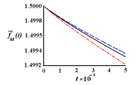
Figure 3: The massive neutrino magnetic form factor versus squared transverse momentum in different gauges. The dashed line corresponds to $\alpha=100$, the solid line to the t’Hooft-Feynman gauge ($\alpha=1$), and the dash-dotted line to $\alpha=0.1$

It can be seen that the magnetic form factor becomes gauge independent at $t=0$ that amounts to the case of on-shell photon. The value $f_{M}(t=0)$ is equal to the neutrino magnetic moment, and Fig. 3 shows gauge independence of this quantity in agreement with our exact calculations performed above.

V Conclusion

We have considered the massive neutrino electric charge and magnetic moment within the context of the standard model supplied with $\mathrm{SU}(2)$-singlet right-handed neutrino in general $R_{\xi}$ gauge. Using the dimensional-regularization scheme, we have calculated the one-loop contributions to the neutrino electromagnetic vertex function taking exactly into account the neutrino mass. We have presented the results of our calculations of different contributions to the neutrino electric charge and magnetic moment as the closed integral expressions. It has allowed us to determine the dependencies of these contributions on the neutrino and corresponding charged lepton masses as well as on the gauge-fixing parameters. The integral expressions for the neutrino electric charge and magnetic moment obtained in this work contain at most two definite integrals which, in principle, can be performed and expressed in terms of elementary functions. However, the results are quite cumbersome and therefore we have presented them as the expansion over the neutrino mass parameter $b$. For several diagrams, which contribute to the neutrino charge and magnetic moment and which have been calculated in Ref. Cabral-Rosetti et al. (2000) with mistakes, we have found the correct results.

We have found the general expressions for the contributions to neutrino electric form factor. These formulae have been derived in general $R_{\xi}$ gauge and at arbitrary value of $q^{2}$. We have shown that the electric charge of a massive neutrino is a gauge independent and vanishing parameter in the first two orders of the expansion over the neutrino mass parameter $b$. In the particular choice of the ’t Hooft-Feynman gauge we have also demonstrated that the neutrino charge is zero in all orders of expansion over $b$, i.e. for arbitrary mass of neutrino. In the previously published works devoted to the calculation of the neutrino electric charge the case of massless neutrino was studied within the Georgi-Glashow (see Ref. Fujikawa et al. (1972)) and Weinberg-Salam (see Refs. Bardeen et al. (1972); Marciano and Sirlin (1980); Sakakibara (1981); Lucio Martínez et al. (1984)) models. However, it is clear that the massless particle must be electrically neutral. Although there is no doubt that the massive neutrino electric charge must be also zero, however it has not been yet shown how it actually happens for corresponding Feynman diagrams.

There are other reasons to prove by the direct calculations that the value of the massive neutrino electric charge is zero. For example, this problem is important in consideration of the neutrino spin oscillations. In the series of our works Egorov et al. (2000); Lobanov and Studenikin (2001); Dvornikov and Studenikin (2002); Lobanov and Studenikin (2003) we have elaborated the quasi-classical approach for the description of the neutrino spin oscillations in arbitrary external electromagnetic field. An essential point in that studies has been the zero charge of the massive neutrino. In this paper we have substantiated this assumption.

From the obtained closed two-integral expression for the massive neutrino electric form factor it is also possible to derive the neutrino charge radius.

The structure of the massive neutrino electromagnetic vertex function have been examined in this work. We have directly verified the decomposition of the neutrino vertex function. It has been found out that the value of the additional ”form factor” $f_{5}(q^{2})$, which is proportional to $\gamma_{\mu}\gamma_{5}$ matrix, at $q^{2}=0$ is zero in the first two orders of the expansion over the neutrino mass parameter $b$ and for arbitrary gauge parameter $\alpha$. The vanishing of the additional ”form factor” $f_{5}(q^{2})$ in the particular gauge ($\alpha_{Z}=\infty$ and $\alpha_{W}=1$) but for the arbitrary charged lepton $a$ and neutrino $b$ mass parameters as well as for arbitrary $q^{2}$ has also been demonstrated. Such direct calculations have never been carried out before.

For each of the diagrams contributing to the neutrino magnetic moment, we have obtained the expressions accounting for the leading (zeroth) and next-to-leading (first) orders in the neutrino mass parameter $b$ with the gauge dependence shown explicitly. Each of the contributions is finite and the sum of all contributions turns out to be gauge-independent. Our calculations also enable us to get the neutrino magnetic moment in the following ranges of the neutrino, charged lepton, and $W$ boson masses: $m_{\nu}\ll m_{\ell}\ll M_{W}$, $m_{\ell}\ll m_{\nu}\ll M_{W}$, and $m_{\ell}\ll M_{W}\ll m_{\nu}$, which span almost all the cases presently discussed within different theoretical models. We have also presented the general formulae for the massive neutrino magnetic form factor at arbitrary $q^{2}$.

As for the behavior of the neutrino magnetic form factor at $q^{2}{\not=}0$, we have found that the function $f_{M}(q^{2})$ essentially depends on the gauge fixing parameter $\alpha$ at $q^{2}{\not=}0$. The magnetic form factor may depend on the gauge parameter at $q^{2}{\not=}0$ since it is not a measurable property of a particle and, therefore, may not be invariant under the gauge group transformations. The consideration of the gauge parameter dependence of the neutrino magnetic form factor as well as its asymptotic behavior at large negative $q^{2}$ in the limit $b\to 0$ within the Weinberg-Salam model is presented in Ref. Fujikawa et al. (1972). The transition magnetic moment of the Dirac neutrinos coupled with the light fermion $f$ ($m_{f}\approx m_{\nu}$) and with the light scalar boson $\phi$ ($m_{\phi}\ll m_{\nu}-m_{f}$) through the Yukawa interaction $\bar{\nu}f\phi$ is discussed in Ref. Frère et al. (1997). The transition magnetic moment dependence on $q^{2}$ is also considered there. The analysis of the neutrino magnetic moment is presented in Ref. Czakon et al. (1999) for various versions of the left-right symmetric models. The results of our massive neutrino magnetic moment calculations can be applied to the treatment of the magnetic moment (including the transitional magnetic moment) within the left-right symmetric model.

Although we have not studied the neutrino anapole form factor in this paper, this particular problem (which we discuss in DvoStuUP) is also important since, for instance, the anapole moment (the value of the anapole form factor at $q^{2}=0$) is the only static electromagnetic property of a Majorana neutrino (see, for instance, Refs. Kayser (1982); Dubovik and Kuznetsov (1998)). It should be noted that even a massless particle can posses the anapole moment, unlike the magnetic moment. Some resent papers are worth mentioning in this respect (see Bukina et al. (1998); Rosado (2000) and references therein). However, the investigation of the neutrino anapole moment faces serious difficulties such as its observability and gauge dependence.

Appendix A Feynman Rules

In this Appendix we present the full list of the Feynman rules Aoki et al. (1982) necessary for the calculation of the massive neutrino electromagnetic vertex. In the $R_{\xi}$ gauge the propagators for the vector bosons, $W$ and $Z$, an unphysical charged scalar boson, $\chi$, as well as charged ghosts, $c$ and $\bar{c}$, are presented in the following form

$$D_{\mu\nu}^{(W)}(k) =\frac{1}{k^{2}-M_{W}^{2}+i\epsilon}\left[g_{\mu\nu}-(1-\alpha)\frac{k_{\mu}k_{\nu}}{k^{2}-\alpha M_{W}^{2}+i\epsilon}\right],$$

$$D_{\mu\nu}^{(Z)}(k) =\frac{1}{k^{2}-M_{Z}^{2}+i\epsilon}\left[g_{\mu\nu}-(1-\alpha_{Z})\frac{k_{\mu}k_{\nu}}{k^{2}-\alpha_{Z}M_{Z}^{2}+i\epsilon}\right],$$

$$D^{(\chi)}(k)=\frac{1}{\alpha M_{W}^{2}-k^{2}-i\epsilon},\quad D^{(c)}(k)=D^{(\overline{c})}(k)=\frac{1}{\alpha M_{W}^{2}-k^{2}-i\epsilon}.$$

The fermion propagator has the standard form

$$S(k)=\frac{{\not k}+m_{n}}{m_{n}^{2}-k^{2}-i\epsilon},$$

where $n$ denotes the type of a fermion.

All vertices can be divided into several classes. We append below the corresponding graphs and Feynman rules for each of these classes.

(a) $g\cos\theta_{W}\{(k-p)^{\gamma}g^{\alpha\beta}+$ $(p-q)^{\alpha}g^{\beta\gamma}+(q-k)^{\beta}g^{\gamma\alpha}\}$

(b) $e\{(k-p)^{\gamma}g^{\alpha\beta}+$ $(p-q)^{\alpha}g^{\beta\gamma}+(q-k)^{\beta}g^{\gamma\alpha}\}$

Figure 4: 4(a)-4(b) vector boson triplex vertices.

(a) $eg\cos\theta_{W}\times$ $\{g^{\alpha\gamma}g^{\beta\delta}+g^{\alpha\delta}g^{\beta\gamma}-2g^{\alpha\beta}g^{\gamma\delta}\}$

Figure 5: 5(a) vector boson quadruple vertex.

(a) $(g/\sqrt{2})\gamma_{\alpha}^{L}$

(b) $(g/\sqrt{2})\gamma_{\alpha}^{L}$

(c) $eQ_{n}\gamma_{\alpha}^{L}$, $n=i$, $I$

(d) $(g/2\cos\theta_{W})\gamma_{\alpha}\times$ $\big{(}1/2-2Q_{I}\sin^{2}\theta_{W}+\gamma_{5}/2\big{)}$

(e) $-(g/2\cos\theta_{W})\gamma_{\alpha}\times$ $\big{(}1/2+2Q_{i}\sin^{2}\theta_{W}+\gamma_{5}/2\big{)}$

Figure 6: 6(a)-6(e) one vector boson and two fermions vertices.

(a) $-(g/2\cos\theta_{W})\times$ $\cos 2\theta_{W}(p-q)_{\alpha}$

(b) $-e(p-q)_{\alpha}$

Figure 7: 7(a)-7(b) one vector boson and two scalar bosons vertices.

(a) $ig\sin^{2}\theta_{W}M_{Z}g_{\alpha\beta}$

(b) $-ieM_{W}g_{\alpha\beta}$

(c) $-ig\sin^{2}\theta_{W}M_{Z}g_{\alpha\beta}$

(d) $ieM_{W}g_{\alpha\beta}$

Figure 8: 8(a)-8(d) two vector bosons and one scalar boson vertices.

(a) $-i(g/\sqrt{2}M_{W})\times$ $(m_{i}P_{R}-m_{I}P_{L})$

(b) $-i(g/\sqrt{2}M_{W})\times$ $(m_{I}P_{R}-m_{i}P_{L})$

Figure 9: 9(a)-9(b) one scalar boson and two fermions vertices.

(a) $-g\cos\theta_{W}p_{\alpha}$

(b) $g\cos\theta_{W}p_{\alpha}$

(c) $-ep_{\alpha}$

(d) $ep_{\alpha}$

Figure 10: 10(a)-10(d) one vector boson and two charged ghosts vertices.

(a) $eg\thinspace g_{\alpha\beta}\times$ $\cos 2\theta_{W}/\cos\theta_{W}$

Figure 11: 11(a) two vector bosons and two scalar bosons vertex.

All the momenta of particles associated with vertices are taken to flow in. $Q_{i,I}$ represent electromagnetic charges of the fields $\psi_{i,I}$ in the units of $e$. $\psi_{i,I}$ representing the three generations of leptons and quarks correspond to usual ”up” (all types of neutrinos as well as $u$, $c$ and $t$ quarks; $I_{3}=+1/2$) and ”down” (all types of leptons as well as $d$, $s$ and $b$ quarks; $I_{3}=-1/2$) components of an isodoublet, respectively, $I_{3}$ is the third component of the isospin.

The arrow on a line indicates the direction of the flow of a certain quantum number: the charge for $W^{\pm}$, $\chi^{\pm}$, the fermion number for $\psi$, the ghost number for $c$, $\overline{c}$. The symbol $\oplus$ or $\ominus$ at the charged ghost lines stands for the sign of the charge carried by the arrow.

Appendix B Feynman integrals

In our calculation of Feynman integrals over virtual momenta we use dimensional-regularization scheme with the following natural properties of $\gamma$-matrix algebra:

$$\{\gamma_{\mu},\gamma_{5}\}=0,\quad\{\gamma_{\mu},\gamma_{\nu}\}=2g_{\mu\nu},\quad g^{\mu\nu}g_{\mu\nu}=N,$$

where $N=4-2\varepsilon$ is the number of dimensions.

The dimensional regularization of the loop integrals in the Euclidian space is performed in the following way:

$$\frac{1}{(2\pi)^{4}}\int d^{4}k\to\frac{1}{(2\pi)^{N}}\int d^{N}k\equiv\frac{\lambda^{2\varepsilon}}{(2\pi)^{N}}\int\limits_{\Omega(N)}d\bm{\Omega}\int\limits_{0}^{\infty}k^{N-1}dk,$$

where $\Omega(N)=2\pi^{N/2}/\Gamma(N/2)$ is the area of a unit sphere in $N$ dimensions. The dependence of an arbitrary positive parameter $\lambda$, which has the mass dimensionality, is introduced to provide the total dimensionality of an integral. The general technique for calculation of various loop integrals in the dimensional regularization scheme can be found, for example, in Ref. Bogoliubov and Shirkov (1980). It should be, however, rather helpful to include here some of the typical loop integrals which one encounters while calculating the electromagnetic vertex function,

$$F_{L}^{(0)}={\frac{i}{\pi^{2}}}\int d^{N}k{\frac{1}{(k^{2}+X)^{L}}}=-\left({\frac{\lambda^{2}i^{2}}{\pi}}\right)^{\varepsilon}{\frac{\Gamma(L-2+\varepsilon)}{\Gamma(L)}}{\frac{1}{X^{L-2+\varepsilon}}},$$

$$F_{1}^{(0)}=X\left[{\frac{1}{\varepsilon}}-\ln\left(-{\frac{\pi X}{\lambda^{2}}}\right)-{\mathbb{C}}+1\right],\quad F_{2}^{(0)}=-{\frac{1}{\varepsilon}}+\ln\left(-{\frac{\pi X}{\lambda^{2}}}\right)+{\mathbb{C}},$$

$$F_{3}^{(0)}=-{\frac{1}{2X}},\quad F_{4}^{(0)}=-{\frac{1}{6X^{2}}},\quad F_{5}^{(0)}=-{\frac{1}{12X^{3}}},$$

$$F_{L}^{(1)}={\frac{i}{\pi^{2}}}\int d^{N}k{\frac{k^{2}}{(k^{2}+X)^{L}}}=\left({\frac{\lambda^{2}i^{2}}{\pi}}\right)^{\varepsilon}{\frac{\Gamma(L-3+\varepsilon)}{\Gamma(L)}}{\frac{\varepsilon-2}{X^{L-3+\varepsilon}}},$$

$$F_{2}^{(1)}=2X\left[{\frac{1}{\varepsilon}}-\ln\left(-{\frac{\pi X}{\lambda^{2}}}\right)-{\mathbb{C}}+{\frac{1}{2}}\right],\quad F_{3}^{(1)}=-{\frac{1}{\varepsilon}}+\ln\left(-{\frac{\pi X}{\lambda^{2}}}\right)+{\mathbb{C}}+{\frac{1}{2}},$$

$$F_{4}^{(1)}=-{\frac{1}{3X}},\quad F_{5}^{(1)}=-{\frac{1}{12X^{2}}},$$

$$F_{L}^{(2)}={\frac{i}{\pi^{2}}}\int d^{N}k{\frac{(k^{2})^{2}}{(k^{2}+X)^{L}}}=-\left({\frac{\lambda^{2}i^{2}}{\pi}}\right)^{\varepsilon}{\frac{\Gamma(L-4+\varepsilon)}{\Gamma(L)}}{\frac{(\varepsilon-2)(\varepsilon-3)}{X^{L-4+\varepsilon}}},$$

$$F_{3}^{(2)}=3X\left[{\frac{1}{\varepsilon}}-\ln\left(-{\frac{\pi X}{\lambda^{2}}}\right)-{\mathbb{C}}+{\frac{1}{6}}\right],\quad F_{4}^{(2)}=-{\frac{1}{\varepsilon}}+\ln\left(-{\frac{\pi X}{\lambda^{2}}}\right)+{\mathbb{C}}+{\frac{5}{6}},$$

$$F_{5}^{(2)}=-{\frac{1}{4X}},$$

where $\mathbb{C}\approx 0.5772157$ is the Euler constant.

References

• Bilenky et al. (2003) S. M. Bilenky, C. Giunti, J. A. Grifols, and E. Masso, Phys. Rep. 379, 69 (2003), eprint hep-ph/0211462.
• Kim (1976) J. E. Kim, Phys. Rev. D 14, 3000 (1976).
• Bég et al. (1978) M. A. B. Bég, W. J. Marciano, and M. Ruderman, Phys. Rev. D 17, 1395 (1978).
• Kayser (1982) B. Kayser, Phys. Rev. D 26, 1662 (1982).
• Lee and Shrock (1977) B. W. Lee and R. E. Shrock, Phys. Rev. D 16, 1444 (1977).
• Bardeen et al. (1972) W. Bardeen, R. Gastmans, and B. Lautrup, Nucl. Phys. B 46, 319 (1972).
• Marciano and Sirlin (1980) W. J. Marciano and A. Sirlin, Phys. Rev. D 22, 2695 (1980).
• Sakakibara (1981) S. Sakakibara, Phys. Rev. D 24, 1149 (1981).
• Lucio Martínez et al. (1984) J. L. Lucio Martínez, A. Rosado, and A. Zepeda, Phys. Rev. D 29, 1539 (1984).
• Fujikawa and Shrock (1980) K. Fujikawa and R. E. Shrock, Phys. Rev. Lett. 45, 963 (1980).
• Shrock (1982) R. E. Shrock, Nucl. Phys. B 206, 359 (1982).
• Egorov et al. (1999) A. M. Egorov, A. E. Lobanov, and A. I. Studenikin, in New Worlds in Astroparticle Physics, edited by A. M. Mourão, M. Pimento, and P. M. Sá (World Scientific, Singapore, 1999), p. 153, eprint hep-ph/9902417.
• Denner et al. (1995) A. Denner, G. Weiglein, and S. Dittmaier, Nucl. Phys. B 440, 95 (1995).
• Cabral-Rosetti et al. (2000) L. G. Cabral-Rosetti, J. Bernabéu, J. Vidal, and A. Zepeda, Eur. Phys. J. C 12, 633 (2000), eprint hep-ph/9907249.
• Acciarri et al. (1999) M. Acciarri et al., Phys. Lett. B 461, 397 (1999), eprint hep-ex/9909006.
• Rosado (2000) A. Rosado, Phys. Rev. D 61, 013001 (2000).
• Wei (1996a) p. 500, in Weinberg (1996) (1996a).
• Lucio et al. (1985) J. L. Lucio, A. Rosado, and A. Zepeda, Phys. Rev. D 31, 1091 (1985).
• Bernabéu et al. (2000) J. Bernabéu, L. G. Cabral-Rosetti, J. Papavassiliou, and J. Vidal, Phys. Rev. D 62, 113012 (2000), eprint hep-ph/0008114.
• Fujikawa et al. (1972) K. Fujikawa, B. W. Lee, and A. I. Sanda, Phys. Rev. D 6, 2923 (1972).
• Wei (1996b) pp. 505–507, in Weinberg (1996) (1996b).
• Egorov et al. (2000) A. Egorov, A. Lobanov, and A. Studenikin, Phys. Lett. B 491, 137 (2000), eprint hep-ph/9910476.
• Lobanov and Studenikin (2001) A. E. Lobanov and A. I. Studenikin, Phys. Lett. B 515, 94 (2001), eprint hep-ph/0106101.
• Dvornikov and Studenikin (2002) M. Dvornikov and A. Studenikin, J. High Energy Phys. 09, 016 (2002), eprint hep-ph/0202113.
• Lobanov and Studenikin (2003) A. Lobanov and A. Studenikin, Phys. Lett. B 564, 27 (2003), eprint hep-ph/0212393.
• Frère et al. (1997) J.-M. Frère, R. B. Nevzorov, and M. I. Vysotsky, Phys. Lett. B 394, 127 (1997), eprint hep-ph/9608266.
• Czakon et al. (1999) M. Czakon, J. Gluza, and M. Zralek, Phys. Rev. D 59, 013010 (1999), eprint hep-ph/9811477.
• Dubovik and Kuznetsov (1998) V. Dubovik and V. Kuznetsov, Int. J. Mod. Phys. A 13, 5257 (1998), eprint hep-ph/9606258.
• Bukina et al. (1998) E. Bukina, V. Dubovik, and V. Kuznetsov, Phys. At. Nucl. 61, 1035 (1998), Yad. Fiz. 61, 1129 (1998).
• Aoki et al. (1982) K. Aoki, Z. Hioki, R. Kawabe, M. Konuma, and T. Muta, Suppl. to the Progr. Theor. Phys. 73, 1 (1982).
• Bogoliubov and Shirkov (1980) N. N. Bogoliubov and D. V. Shirkov, Introduction to theory of quantized fields (Wiley, New York, 1980), 3rd ed.
• Weinberg (1996) S. Weinberg, The quantum theory of fields (Cambridge University Press, 1996), vol. 1, 2nd ed.