Simple Atoms, Quantum Electrodynamics
and Fundamental Constants

Abstract

This review is devoted to precision physics of simple atoms. The atoms can essentially be described in the framework of quantum electrodynamics (QED), however, the energy levels are also affected by the effects of the strong interaction due to the nuclear structure. We pay special attention to QED tests based on studies of simple atoms and consider the influence of nuclear structure on energy levels. Each calculation requires some values of relevant fundamental constants. We discuss the accurate determination of the constants such as the Rydberg constant, the fine structure constant and masses of electron, proton and muon etc.

1 Introduction

Simple atoms offer an opportunity for high accuracy calculations within the framework of quantum electrodynamics (QED) of bound states. Such atoms also possess a simple spectrum and some of their transitions can be measured with high precision. Twenty, thirty years ago most of the values which are of interest for the comparison of theory and experiment were known experimentally with a higher accuracy than from theoretical calculations. After a significant theoretical progress in the development of bound state QED, the situation has reversed. A review of the theory of light hydrogen-like atoms can be found in report , while recent advances in experiment and theory have been summarized in the Proceedings of the International Conference on Precision Physics of Simple Atomic Systems (2000) book .

Presently, most limitations for a comparison come directly or indirectly from the experiment. Examples of a direct experimental limitation are the $1s-2s$ transition and the $1s$ hyperfine structure in positronium, whose values are known theoretically better than experimentally. An indirect experimental limitation is a limitation of the precision of a theoretical calculation when the uncertainty of such calculation is due to the inaccuracy of fundamental constants (e.g. of the muon-to-electron mass ratio needed to calculate the $1s$ hyperfine interval in muonium) or of the effects of strong interactions (like e.g. the proton structure for the Lamb shift and $1s$ hyperfine splitting in the hydrogen atom). The knowledge of fundamental constants and hadronic effects is limited by the experiment and that provides experimental limitations on theory.

This is not our first brief review on simple atoms (see e.g. icap ; limits ) and to avoid any essential overlap with previous papers, we mainly consider here the most recent progress in the precision physics of hydrogen-like atoms since the publication of the Proceedings book . In particular, we discuss

• Lamb shift in the hydrogen atom;

• hyperfine structure in hydrogen, deuterium and helium ion;

• hyperfine structure in muonium and positronium;

• $g$ factor of a bound electron.

We consider problems related to the accuracy of QED calculations, hadronic effects and fundamental constants.

These atomic properties are of particular interest because of their applications beyond atomic physics. Understanding of the Lamb shift in hydrogen is important for an accurate determination of the Rydberg constant $Ry$ and the proton charge radius. The hyperfine structure in hydrogen, helium-ion and positronium allows, under some conditions, to perform an accurate test of bound state QED and in particular to study some higher-order corrections which are also important for calculating the muonium hyperfine interval. The latter is a source for the determination of the fine structure constant $\alpha$ and muon-to-electron mass ratio. The study of the $g$ factor of a bound electron lead to the most accurate determination of the proton-to-electron mass ratio, which is also of interest because of a highly accurate determination of the fine structure constant.

2 Rydberg Constant and Lamb Shift in Hydrogen

About fifty years ago it was discovered that in contrast to the spectrum predicted by the Dirac equation, there are some effects in hydrogen atom which split the $2s_{1/2}$ and $2p_{1/2}$ levels. Their splitting known as the Lamb shift (see Fig. 1) was successfully explained by quantum electrodynamics. The QED effects lead to a tiny shift of energy levels and for thirty years this shift was studied by means of microwave spectroscopy (see e.g. hinds ; pipkin ) measuring either directly the splitting of the $2s_{1/2}$ and $2p_{1/2}$ levels or a bigger splitting of the $2p_{3/2}$ and $2s_{1/2}$ levels (fine structure) where the QED effects are responsible for approximately 10% of the fine-structure interval.

Figure 1: Spectrum of the hydrogen atom (not to scale). The hyperfine structure is neglected. The label rf stands for radiofrequency intervals, while uv is for ultraviolet transitions

The recent success of two-photon Doppler-free spectroscopy twophot opens another way to study QED effects directed by high-resolution spectroscopy of gross-structure transitions. Such a transition between energy levels with different values of the principal quantum number $n$ is determined by the Coulomb-Schrödinger formula

$$E(nl)=-\frac{(Z\alpha)^{2}mc^{2}}{2n^{2}}\;,$$ (1)

where $Z$ is the nuclear charge in units of the proton charge, $m$ is the electron mass, $c$ is the speed of light, and $\alpha$ is the fine structure constant. For any interpretation in terms of QED effects one has to determine a value of the Rydberg constant

$$Ry=\frac{\alpha^{2}mc}{2h}\;,$$ (2)

where $h$ is the Planck constant. Another problem in the interpretation of optical measurements of the hydrogen spectrum is the existence of a few levels which are significantly affected by the QED effects. In contrast to radiofrequency measurements, where the $2s-2p$ splitting was studied, optical measurements have been performed with several transitions involving $1s$, $2s$, $3s$ etc. It has to be noted that the theory of the Lamb shift for levels with $l\neq 0$ is relatively simple, while theoretical calculations for $s$ states lead to several serious complifications. The problem of the involvement of few $s$ levels has been solved by introducing an auxiliary difference del1

$$\Delta(n)=E_{L}(1s)-n^{3}E_{L}(ns)\;,$$ (3)

for which theory is significantly simpler and more clear than for each of the $s$ states separately.

Combining theoretical results for the difference del2 with measured frequencies of two or more transitions one can extract a value of the Rydberg constant and of the Lamb shift in the hydrogen atom. The most recent progress in determination of the Rydberg constant is presented in Fig. 2 (see twophot ; codata for references).

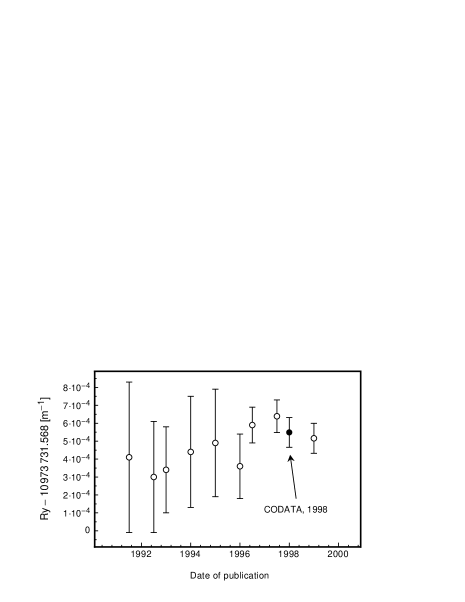
Figure 2: Progress in the determination of the Rydberg constant by two-photon Doppler-free spectroscopy of hydrogen and deuterium. The label CODATA, 1998 stands for the recommended value of the Rydberg constant ($Ry=10\,973\,731.568\,549(83)\;$m^-1 [10])

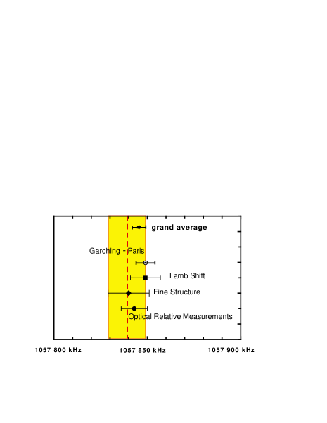
Figure 3: Measurement of the Lamb shift in hydrogen atom. Theory is presented according to [11]. The most accurate value comes from comparison of the $1s-2s$ transition at MPQ (Garching) and the $2s-ns/d$ at LKB (Paris), where $n=8,10,12$. Three results are shown: for the average values extracted from direct Lamb shift measurements, measurements of the fine structure and a comparison of two optical transitions within a single experiment. The filled part is for the theory

Presently the optical determination twophot ; limits of the Lamb shift in the hydrogen atom dominates over the microwave measurements hinds ; pipkin . The extracted value of the Lamb shift has an uncertainty of 3 ppm. That ought to be compared with the uncertainty of QED calculations (2 ppm) rp and the uncertainty of the contributions of the nuclear effects. The latter has a simple form

$$\Delta E_{\rm charge~{}radius}(nl)=\frac{2(Z\alpha)^{4}mc^{2}}{3n^{3}}\,\left(\frac{mcR_{p}}{\hbar}\right)^{2}\,\delta_{l0}\;.$$ (4)

To calculate this correction one has to know the proton rms charge radius $R_{p}$ with sufficient accuracy. Unfortunately, it is not known well enough rp ; icap and leads to an uncertainty of 10 ppm for the calculation of the Lamb shift. It is likely that a result for $R_{p}$ from the electron-proton elastic scattering mainz cannot be improved much, but it seems to be possible to significantly improve the accuracy of the determination of the proton charge radius from the Lamb-shift experiment on muonic hydrogen, which is now in progress at PSI psi .

3 Hyperfine Structure and Nuclear Effects

A similar problem of interference of nuclear structure and QED effects exists for the $1s$ and $2s$ hyperfine structure in hydrogen, deuterium, tritium and helium-3 ion. The magnitude of nuclear effects entering theoretical calculations is at the level from 30 to 200 ppm (depending on the atom) and their understanding is unfortunately very poor rp ; khr ; d21 . We summarize the data in Tables 1 and 2 (see d21 for detail).

Atom,	$E_{\rm HFS}({\rm exp})$	Ref.	$E_{\rm HFS}({\rm QED})$	$\Delta E({\rm Nucl})$
state	[kHz]		[kHz]	[ppm]
Hydrogen, $1s$	1 420 405.751 768(1)	cjp2000 ; exph1s	1 420 452	- 33
Deuterium, $1s$	327 384.352 522(2)	expd1s	327 339	138
Tritium, $1s$	1 516 701.470 773(8)	mathur	1 516 760	- 36
3He+ ion, $1s$	- 8 665 649.867(10)	exphe1s	- 8 667 494	- 213
Hydrogen, $2s$	177 556.860(15)	2shydr+ ; 2shydr	177 562.7	-32
Hydrogen, $2s$	177 556.785(29)	rothery		- 33
Hydrogen, $2s$	177 556.860(50)	exph2s		- 32
Deuterium, $2s$	40 924.439(20)	expd2s	40 918.81	137
3He+ ion, $2s$	- 1083 354.980 7(88)	prior	- 1083 585.3	- 213
3He+ ion, $2s$	- 1083 354.99(20)	exphe2s		- 213

Table 1: Hyperfine structure in light hydrogen-like atoms: QED and nuclear contributions $\Delta E({\rm Nucl})$. The numerical results are presented for the frequency $E/h$

The leading term (so-called Fermi energy $E_{F}$) is a result of the nonrelativistic interaction of the Dirac magnetic moment of electron with the actual nuclear magnetic moment. The leading QED contribution is related to the anomalous magnetic moment and simply rescales the result ($E_{F}\to E_{F}\cdot(1+a_{e})$). The result of the QED calculations presented in Table 1 is of the form

$$E_{\rm HFS}({\rm QED})=E_{F}\cdot(1+a_{e})+\Delta E({\rm QED})\;,$$ (5)

where the last term which arises from bound-state QED effects for the $1s$ state is given by

$$\Delta E_{1s}({\rm QED})=E_{F} \times \left\{\frac{3}{2}(Z\alpha)^{2}+\alpha(Z\alpha)\left(\ln 2-\frac{5}{2}\right)\right.$$ (6)

$$+ {\alpha(Z\alpha)^{2}\over\pi}\left[-\frac{2}{3}\ln{1\over(Z\alpha)^{2}}\left(\ln{\frac{1}{(Z\alpha)^{2}}}\right.\right.$$ (7)

$$+ \left.4\ln 2-\frac{281}{240}\right)+17.122\,339\ldots$$ (8)

$$- \left.\left.\frac{8}{15}\ln{2}+\frac{34}{225}\right]+0.7718(4)\,\frac{\alpha^{2}(Z\alpha)}{\pi}\right\}\,.$$ (9)

This term is in fact smaller than the nuclear corrections as it is shown in Table 2 (see d21 for detail). A result for the $2s$ state is of the same form with slightly different coeffitients d21 .

Atom	$\Delta E({\rm QED})$	$\Delta E({\rm Nucl})$
	[ppm]	[ppm]
Hydrogen	23	- 33
Deuterium	23	138
Tritium	23	- 36
3He+ ion	108	- 213

Table 2: Comparison of bound QED and nuclear corrections to the $1s$ hyperfine interval. The QED term $\Delta E({\rm QED})$ contains only bound-state corrections and the contribution of the anomalous magnetic moment of electron is excluded. The nuclear contribution $\Delta E({\rm Nucl})$ has been found via comparison of experimental results with pure QED values (see Table 1)

From Table 1 one can learn that in relative units the effects of nuclear structure are about the same for the $1s$ and $2s$ intervals (33 ppm for hydrogen, 138 ppm for deuterium and 213 ppm for helium-3 ion). A reason for that is the factorized form of the nuclear contributions in leading approximation (cf. (4))

$$\Delta E({\rm Nucl})=A({\rm Nucl})\times\big{|}\Psi_{nl}({\bf r}=0)\big{|}^{2}\;$$ (10)

i.e. a product of the nuclear-structure parameter $A({\rm Nucl})$ and a the wave function at the origin

$$\big{|}\Psi_{nl}({\bf r}=0)\big{|}^{2}=\frac{1}{\pi}\left(\frac{(Z\alpha)m_{R}c}{n\hbar}\right)^{3}\delta_{l0}\;,$$ (11)

which is a result of a pure atomic problem (a nonrelativistic electron bound by the Coulomb field). The nuclear parameter $A({\rm Nucl})$ depends on the nucleus (proton, deutron etc.) and effect (hyperfine structure, Lamb shift) under study, but does not depend on the atomic state.

Two parameters can be changed in the wave function:

• the principle quantum number $n=1,2$ for the $1s$ and $2s$ states;

• the reduced mass of a bound particle for conventional (electronic) atoms ($m_{R}\simeq m_{e}$) and muonic atoms ($m_{R}\simeq m_{\mu}$).

The latter option was mentioned when considering determination of the proton charge radius via the measurement of the Lamb shift in muonic hydrogen psi . In the next section we consider the former option, comparison of the $1s$ and $2s$ hyperfine interval in hydrogen, deuterium and ion ³He⁺.

4 Hyperfine Structure of the $2s$ State in Hydrogen, Deuterium and Helium-3 Ion

Our consideration of the $2s$ hyperfine interval is based on a study of the specific difference

$$D_{21}=8\cdot E_{\rm HFS}(2s)-E_{\rm HFS}(1s)\;,$$ (12)

where any contribution which has a form of (10) should vanish.

Contribution	Hydrogen	Deuterium	3He+ ion
	[kHz]	[kHz]	[kHz]
$D_{21}({\rm QED3})$	48.937	11.305 6	-1 189.252
$D_{21}({\rm QED4})$	0.018(3)	0.004 3(5)	-1.137(53)
$D_{21}({\rm nucl})$	-0.002	0.002 6(2)	0.317(36)
$D_{21}({\rm theo})$	48.953(3)	11.312 5(5)	-1 190.072(63)

Table 3: Theory of the specific difference $D_{21}=8E_{\rm HFS}(2s)-E_{\rm HFS}(1s)$ in light hydrogen-like atoms (see [15] for detail). The numerical results are presented for the frequency $D_{21}/h$

The difference (12) has been studied theoretically in several papers long ago zwanziger ; sternheim ; pmohr . A recent study sgkH2s shown that some higher-order QED and nuclear corrections have to be taken into account for a proper comparison of theory and experiment. The theory has been substantially improved d21 ; yero2001 and it is summarized in Table 3. The new issues here are most of the fourth-order QED contributions ($D_{21}({\rm QED4})$) of the order $\alpha(Z\alpha)^{3}$, $\alpha^{2}(Z\alpha)^{4}$, $\alpha(Z\alpha)^{2}{m/M}$ and $(Z\alpha)^{3}{m/M}$ (all are in units of the $1s$ hyperfine interval) and nuclear corrections ($D_{21}({\rm nucl})$). The QED corrections up to the third order ($D_{21}({\rm QED3})$) and the fourth-order contribution of the order $(Z\alpha)^{4}$ have been known for a while zwanziger ; sternheim ; pmohr ; 17breit .

Figure 4: Level scheme for an optical measurement of the hyperfine structure (hfs) in the hydrogen atom (not to scale) [22]. The label rf stands here for radiofrequency intervals, while uv is for ultraviolet transitions

For all the atoms in Table 3 the hyperfine splitting in the ground state was measured more accurately than for the $2s$ state. All experimental results but one were obtained by direct measurements of microwave transitions for the $1s$ and $2s$ hyperfine intervals. However, the most recent result for the hydrogen atom has been obtained by means of laser spectroscopy and measured transitions lie in the ultraviolet range 2shydr+ ; 2shydr . The hydrogen level scheme is depicted in Fig. 4. The measured transitions were the singlet-singlet ($F=0$) and triplet-triplet ($F=1$) two-photon $1s-2s$ ultraviolet transitions. The eventual uncertainty of the hyperfine structure is to 6 parts in $10^{15}$ of the measured $1s-2s$ interval. The optical result in Table 1 is a preliminary one and the data analysis is still in progress.

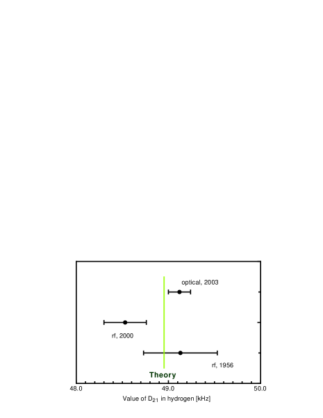
Figure 5: Present status of measurements of $D_{21}$ in the hydrogen atom. The results are labeled with the date of the measurement of the $2s$ hyperfine structure. See Table 1 for references

The comparison of theory and experiment for hydrogen and helium-3 ion is summarized in Figs. 5 and 6.

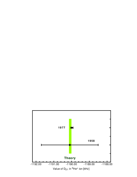
Figure 6: Present status of measurements of $D_{21}$ in the helium ion ³He⁺. See Table 1 for references

5 Hyperfine Structure in Muonium and Positronium

Another possibility to eliminate nuclear structure effects is based on studies of nucleon-free atoms. Such an atomic system is to be formed of two leptons. Two atoms of the sort have been produced and studied for a while with high accuracy, namely, muonium and positronium.

• Muonium is a bound system of a positive muon and electron. It can be produced with the help of accelerators. The muon lifetime is $2.2\cdot 10^{-6}$ sec. The most accurately measured transition is the $1s$ hyperfine structure. The two-photon $1s-2s$ transition was also under study. A detailed review of muonium physics can be found in jungmann .

• Positronium can be produced at accelerators or using radioactive positron sources. The lifetime of positronium depends on its state. The lifetime for the $1s$ state of parapositronium (it annihilates mainly into two photons) is $1.25\cdot 10^{-10}$ sec, while orthopositronium in the $1s$ state has a lifetime of $1.4\cdot 10^{-7}$ s because of three-photon decays. A list of accurately measured quantities contains the $1s$ hyperfine splitting, the $1s-2s$ interval, $2s-2p$ fine structure intervals for the triplet $1s$ state and each of the four $2p$ states, the lifetime of the $1s$ state of para- and orthopositronium and several branchings of their decays. A detailed review of positronium physics can be found in conti .

Term	Fractional	$\Delta E$
	contribution	[kHz]
$E_{F}$	1.000 000 000	4.459 031.83(50)(3)
$a_{e}$	0.001 159 652	5 170.926(1)
QED2	- 0.000 195 815	- 873.147
QED3	- 0.000 005 923	- 26.410
QED4	- 0.000 000 123(49)	- 0.551(218)
Hadronic	0.000 000 054(1)	0.240(4)
Weak	- 0.000 000 015	- 0.065
Total	1.000 957 830(49)	4 463 302.68(51)(3)(22)

Table 4: Theory of the $1s$ hyperfine splitting in muonium. The numerical results are presented for the frequency $E/h$. The calculations [36] have been performed for $\alpha^{-1}=137.035\,999\,58(52)$ [37] and $\mu_{\mu}/\mu_{p}=3.183\,345\,17(36)$ which was obtained from the analysis of the data on Breit-Rabi levels in muonium [38,39] (see Sect. 6) and precession of the free muon [40]. The numerical results are presented for the frequency $E/h$

Term	Fractional	$\Delta E$
	contribution	[MHz]
$E_{F}$	1.000 000 0	204 386.6
QED1	- 0.004 919 6	-1 005.5
QED2	0.000 057 7	11.8
QED3	- 0.000 006 1(22)	- 1.2(5)
Total	0.995 132 1(22)	203 391.7(5)

Table 5: Theory of the $1s$ hyperfine interval in positronium. The numerical results are presented for the frequency $E/h$. The calculation of the second order terms was completed in [41], the leading logarithmic contributions were found in [42], while next-to-leading logarithmic terms in [43]. The uncertainty is presented following [44]

Here we discuss only the hyperfine structure of the ground state in muonium and positronium. The theoretical status is presented in Tables 4 and 5. The theoretical uncertainty for the hyperfine interval in positronium is determined only by the inaccuracy of the estimation of the higher-order QED effects. The uncertainty budget in the case of muonium is more complicated. The biggest source is the calculation of the Fermi energy, the accuracy of which is limited by the knowledge of the muon magnetic moment or muon mass. It is essentially the same because the $g$ factor of the free muon is known well enough redin . The uncertainty related to QED is determined by the fourth-order corrections for muonium ($\Delta E(QED4)$) and the third-order corrections for positronium ($\Delta E(QED3)$). These corrections are related to essentially the same diagrams (as well as the $D_{21}(QED4)$ contribution in the previous section). The muonium uncertainty is due to the calculation of the recoil corrections of the order of $\alpha(Z\alpha)^{2}m/M$ log1 ; log2 and $(Z\alpha)^{3}m/M$, which are related to the third-order contributions log1 for positronium since $m=M$.

The muonium calculation is not completely free of hadronic contributions. They are discussed in detail in hamu1 ; hamu2 ; hamu3 and their calculation is summarized in Fig. 7. They are small enough but their understanding is very important because of the intensive muon sources expected in future sources which might allow to increase dramatically the accuracy of muonium experiments.

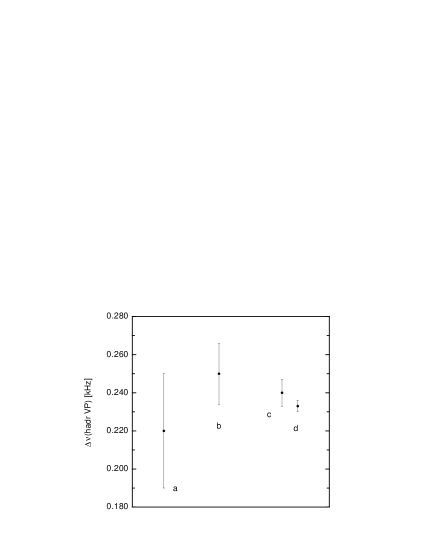
Figure 7: Hadronic contributions to HFS in muonium. The results are taken: $a$ from [50], $b$ from [51], $c$ from [52] and $d$ from [36,47]

A comparison of theory versus experiment for muonium is presented in the summary of this paper. Present experimental data for positronium together with the theoretical result are depicted in Fig. 8.

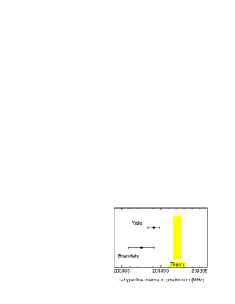
Figure 8: Positronium hyperfine structure. The Yale experiment was performed in 1984 [53] and the Brandeis one in 1975 [54]

6 $g$ Factor of Bound Electron and Muon in Muonium

Not only the spectrum of simple atoms can be studied with high accuracy. Other quantities are accessible to high precision measurements as well among them the atomic magnetic moment. The interaction of an atom with a weak homogeneous magnetic field can be expressed in terms of an effective Hamiltonian. For muonium such a Hamiltonian has the form

$${\cal H}={e\hbar\over 2m_{e}}g^{\prime}_{e}\,\bigl{(}{\bf s}_{e}\cdot{\bf B}\bigr{)}-{e\hbar\over 2m_{N}}g^{\prime}_{\mu}\,\bigl{(}{\bf s}_{\mu}\cdot{\bf B}\bigr{)}+\Delta E_{\rm HFS}\,\bigl{(}{\bf s}_{e}\cdot{\bf s}_{\mu}\bigr{)}\;,$$ (13)

where ${\bf s}_{e(\mu)}$ stands for spin of electron (muon), and $g^{\prime}_{e(\mu)}$ for the $g$ factor of a bound electron (muon) in the muonium atom. The bound $g$ factors are now known up to the fourth-order corrections zee including the term of the order $\alpha^{4}$, $\alpha^{3}m_{e}/m_{\mu}$ and $\alpha^{2}m_{e}/m_{\mu}$ and thus the relative uncertainty is essentially better than $10^{-8}$. In particular, the result for the bound muon $g$ factor reads zee

$$g_{\mu}^{\prime}=g_{\mu}^{(0)}\cdot\biggl{\{} 1 -{\alpha(Z\alpha)\over 3}\left[1-{3\over 2}{m_{e}\over m_{\mu}}\right]$$ (14)

$$- {\alpha(Z\alpha)(1+Z)\over 2}\left({m_{e}\over m_{\mu}}\right)^{2}+{\alpha^{2}(Z\alpha)\over{12\pi}}{m_{e}\over m_{\mu}}-{97\over 108}\,\alpha(Z\alpha)^{3}\biggr{\}},$$ (15)

where $g_{\mu}^{(0)}=2\cdot(1+a_{\mu})$ is the $g$ factor of a free muon. Equation (13) has been applied MuExp ; MuExp1 to determine the muon magnetic moment and muon mass by measuring the splitting of sublevels in the hyperfine structure of the $1s$ state in muonium in a homogeneous magnetic field. Their dependence on the magnetic field is given by the well known Breit-Rabi formula (see e.g. bethe ). Since the magnetic field was calibrated via spin precession of the proton, the muon magnetic moment was measured in units of the proton magnetic moment, and muon-to-electron mass ratio was derived as

$$\frac{m_{\mu}}{m_{e}}=\frac{\mu_{\mu}}{\mu_{p}}\,\frac{\mu_{p}}{\mu_{B}}\,\frac{1}{1+a_{\mu}}\;.$$ (16)

Results on the muon mass extracted from the Breit-Rabi formula are among the most accurate (see Fig. 9). A more precise value can only be derived from the muonium hyperfine structure after comparison of the experimental result with theoretical calculations. However, the latter is of less interest, since the most important application of the precise value of the muon-to-electron mass is to use it as an input for calculations of the muonium hyperfine structure while testing QED or determining the fine structure constants $\alpha$. The adjusted CODATA result in Fig. 9 was extracted from the muonium hyperfine structure studies and in addition used some overoptimistic estimation of the theoretical uncertainty (see hamu1 for detail).

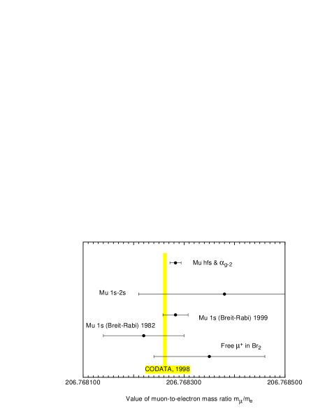
Figure 9: The muon-to-electron mass ratio. The most accurate result obtained from comparison of the measured hyperfine interval in muonium [38] to the theoretical calculation [36] performed with $\alpha_{g-2}^{-1}=137.035\,999\,58(52)$ [37]. The results derived from the Breit-Rabi sublevels are related to two experiments performed at LAMPF in 1982 [39] and 1999 [38]. The others are taken from the measurement of the $1s-2s$ interval in muonium [57], precession of a free muon in bromine [40] and from the CODATA adjustment [10]

7 $g$ Factor of a Bound Electron in a Hydrogen-Like Ion with Spinless Nucleus

In the case of an atom with a conventional nucleus (hydrogen, deuterium etc.) another notation is used and the expression for the Hamiltonian similar to eq. (13) can be applied. It can be used to test QED theory as well as to determine the electron-to-proton mass ratio. We underline that in contrast to most other tests it is possible to do both simultaneously because of a possibility to perform experiments with different ions.

The theoretical expression for the $g$ factor of a bound electron can be presented in the form icap ; sgkH2 ; pla

$$g^{\prime}_{e}=2\cdot\bigl{(}1+a_{e}+b\bigr{)}\;,$$ (17)

where the anomalous magnetic moment of a free electron $a_{e}=0.001\,159\,652\,2$ trap ; codata is known with good enough accuracy and $b$ is the bound correction. The summary of the calculation of the bound corrections is presented in Table 6. The uncertainty of unknown two-loop contributions is taken from gjetp . The calculation of the one-loop self-energy is different for different atoms. For lighter elements (helium, beryllium), it is obtained from zee based on fitting data of beier , while for heavier ions we use the results of oneloop . The other results are taken from gjetp (for the one-loop vacuum polarization), pla (for the nuclear correction and the electric part of the light-by-light scattering (Wichmann-Kroll) contribution), plb2002 (for the magnetic part of the light-by-light scattering contribution) and recoil2 (for the recoil effects).

Ion	$g$
4He+	2.002 177 406 7(1)
10Be3+	2.001 751 574 5(4)
12C5+	2.001 041 590 1(4)
16O7+	2.000 047 020 1(8)
18O7+	2.000 047 021 3(8)

Table 6: The bound electron $g$ factor in low-$Z$ hydrogen-like ions with spinless nucleus

Before comparing theory and experiment, let us shortly describe some details of the experiment. To determine a quantity like the $g$ factor, one needs to measure some frequency at some known magnetic field $B$. It is clear that there is no way to directly determine magnetic field with a high accuracy. The conventional way is to measure two frequencies and to compare them. The frequencies measured in the GSI-Mainz experiment werth are the ion cyclotron frequency

$${\omega_{c}}=\frac{{(Z-1)e}}{M_{i}}B$$ (18)

and the Larmor spin precession frequency for a hydrogen-like ion with spinless nucleus

$${\omega_{L}}={g_{b}}\,\frac{{e}}{2m_{e}}B\;,$$ (19)

where $M_{i}$ is the ion mass.

Combining them, one can obtain a result for the $g$ factor of a bound electron

$$\frac{g_{b}}{2}={\bigl{(}Z-1\bigr{)}}\,\frac{m_{e}}{M_{i}}\,\frac{\omega_{L}}{\omega_{c}}\;$$ (20)

or an electron-to-ion mass ratio

$$\frac{m_{e}}{M_{i}}=\frac{1}{Z-1}\,\frac{g_{b}}{2}\,\frac{\omega_{c}}{\omega_{L}}\;.$$ (21)

Today the most accurate value of ${m_{e}}/{M_{i}}$ (without using experiments on the bound $g$ factor) is based on a measurement of $m_{e}/m_{p}$ realized in Penning trap farnham with a fractional uncertainty of 2 ppm. The accuracy of measurements of $\omega_{c}$ and $\omega_{L}$ as well as the calculation of $g_{b}$ (as shown in sgkH2 ) are essentially better. That means that it is preferable to apply (21) to determine the electron-to-ion mass ratio me . Applying the theoretical value for the $g$ factor of the bound electron and using experimental results for $\omega_{c}$ and $\omega_{L}$ in hydrogen-like carbon werth and some auxiliary data related to the proton and ion masses, from codata , we arrive at the following values

$$\frac{m_{p}}{m_{e}}=1\,836.152\,673\,1(10)$$ (22)

and

$$m_{e}=0.000\,548\,579\,909\,29(31)~{}{\rm u}\;,$$ (23)

which differ slightly from those in me . The present status of the determination of the electron-to-proton mass ratio is summarized in Fig. 10.

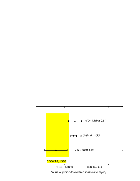
Figure 10: The proton-to-electron mass ratio. The theory of the bound $g$ factor is taken from Table 6, while the experimental data on the $g$ factor in carbon and oxygen are from [68,69]. The Penning trap result from University of Washington is from [66]

In sgkH2 it was also suggested in addition to the determination of the electron mass to check theory by comparing the $g$ factor for two different ions. In such a case the uncertainty related to ${m_{e}}/{M_{i}}$ in (20) vanishes. Comparing the results for carbon werth and oxygen werthcjp , we find

$$g(^{12}{\rm C}^{5+})/g(^{16}{\rm O}^{7+})=1.000\,497\,273\,3(9)$$ (24)

to be compared to the experimental ratio

$$g(^{12}{\rm C}^{5+})/g(^{16}{\rm O}^{7+})=1.000\,497\,273\,1(15)\,.$$ (25)

Theory appears to be in fair agreement with experiment. In particular, this means that we have a reasonable estimate of uncalculated higher-order terms. Note, however, that for metrological applications it is preferable to study lower $Z$ ions (hydrogen-like helium (${}^{4}{\rm He}^{+}$) and beryllium (${}^{10}{\rm Be}^{3+}$)) to eliminate these higher-order terms.

8 The Fine Structure Constant

The fine structure constant plays a basic role in QED tests. In atomic and particle physics there are several ways to determine its value. The results are summarized in Fig. 11. One method based on the muonium hyperfine interval was briefly discussed in Sect. 5. A value of the fine structure constant can also be extracted from the neutral-helium fine structure helium ; heliumexp and from the comparison of theory alphag2 and experiment trap for the anomalous magnetic moment of electron ($\alpha_{g-2}$). The latter value has been the most accurate one for a while and there was a long search for another competitive value. The second value ($\alpha_{Cs}$) on the list of the most precise results for the fine structure constant is a result from recoil spectroscopy chu .

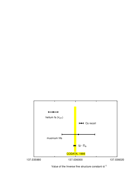
Figure 11: The fine structure constant from atomic physics and QED

We would like to briefly consider the use and the importance of the recoil result for the determination of the fine structure constant. Absorbing and emitting a photon, an atom can gain some kinetic energy which can be determined as a shift of the emitted frequency in respect to the absorbed one ($\delta f$). A measurement of the frequency with high accuracy is the goal of the photon recoil experiment chu . Combining the absorbed frequency and the shifted one, it is possible to determine a value of atomic mass (in chu that was caesium) in frequency units, i.e. a value of $M_{a}c^{2}/h$. That may be compared to the Rydberg constant $Ry=\alpha^{2}m_{e}c/2h$. The atomic mass is known very well in atomic units (or in units of the proton mass) Rain , while the determination of electron mass in proper units is more complicated because of a different order of magnitude of the mass. The biggest uncertainty of the recoil photon value of $\alpha_{\rm Cs}$ comes now from the experiment chu , while the electron mass is the second source.

The success of $\alpha_{\rm Cs}$ determination was ascribed to the fact that $\alpha_{g-2}$ is a QED value being derived with the help of QED theory of the anomalous magnetic moment of electron, while the photon recoil result is free of QED. We would like to emphasize that the situation is not so simple and involvement of QED is not so important. It is more important that the uncertainty of $\alpha_{g-2}$ originates from understanding of the electron behaviour in the Penning trap and it dominates any QED uncertainty. For this reason, the value of $\alpha_{Cs}$ from $m_{p}/m_{e}$ in the Penning trap farnham obtained by the same group as the one that determined the value of the anomalous magnetic moment of electron trap , can actually be correlated with $\alpha_{g-2}$. The result

$$\alpha_{\rm Cs}^{-1}=137.036\,0002\,8(10)$$ (26)

presented in Fig. 11 is obtained using $m_{p}/m_{e}$ from (22). The value of the proton-to-electron mass ratio found this way is free of the problems with an electron in the Penning trap, but some QED is involved. However, it is easy to realize that the QED uncertainty for the $g$ factor of a bound electron and for the anomalous magnetic moment of a free electron are very different. The bound theory deals with simple Feynman diagrams but in Coulomb field and in particular to improve theory of the bound $g$ factor, we need a better understanding of Coulomb effects for “simple” two-loop QED diagrams. In contrast, for the free electron no Coulomb field is involved, but a problem arises because of the four-loop diagrams. There is no correlation between these two calculations.

9 Summary

To summarize QED tests related to hyperfine structure, we present in Table 7 the data related to hyperfine structure of the $1s$ state in positronium and muonium and to the $D_{21}$ value in hydrogen, deuterium and helium-3 ion. The theory agrees with the experiment very well.

Atom	Experiment	Theory	$\Delta/\sigma$	$\sigma/E_{F}$
	[kHz]	[kHz]		[ppm]
Hydrogen, $D_{21}$	49.13(15), 2shydr+ ; 2shydr	48.953(3)	1.2	0.10
Hydrogen, $D_{21}$	48.53(23), rothery		-1.8	0.16
Hydrogen, $D_{21}$	49.13(40), exph2s		0.4	0.28
Deuterium, $D_{21}$	11.16(16), expd2s	11.312 5(5)	-1.0	0.49
3He+ ion, $D_{21}$	-1 189.979(71), prior	-1 190.072(63)	1.0	0.01
3He+, $D_{21}$	-1 190.1(16), exphe2s		0.0	0.18
Muonium, $1s$	4 463 302.78(5)	4 463 302.88(55)	-0.18	0.11
Positronium, $1s$	203 389 100(740)	203 391 700(500)	-2.9	4.4
Positronium, $1s$	203 397 500(1600)		-2.5	8.2

Table 7: Comparison of experiment and theory of hyperfine structure in hydrogen-like atoms. The numerical results are presented for the frequency $E/h$. In the $D_{21}$ case the reference is given only for the $2s$ hyperfine interval

The precision physics of light simple atoms provides us with an opportunity to check higher-order effects of the perturbation theory. The highest-order terms important for comparison of theory and experiment are collected in Table 8. The uncertainty of the $g$ factor of the bound electron in carbon and oxygen is related to $\alpha^{2}(Z\alpha)^{4}m$ corrections in energy units, while for calcium the crucial order is $\alpha^{2}(Z\alpha)^{6}m$.

Some of the corrections presented in Table 8 are completely known, some not. Many of them and in particular $\alpha(Z\alpha)^{6}m^{2}/M^{3}$ and $(Z\alpha)^{7}m^{2}/M^{3}$ for the hyperfine structure in muonium and helium ion, $\alpha^{2}(Z\alpha)^{6}m$ for the Lamb shift in hydrogen and helium ion, $\alpha^{7}m$ for positronium have been known in a so-called logarithmic approximation. In other words, only the terms with the highest power of “big” logarithms (e.g. $\ln(1/Z\alpha)\sim\ln(M/m)\sim 5$ in muonium) have been calculated. This program started for non-relativistic systems in log1 and was developed in log2 ; del1 ; pk2 ; sgkH2s ; d21 . By now even some non-leading logarithmic terms have been evaluated by several groups logps ; morelogs . It seems that we have reached some numerical limit related to the logarithmic contribution and the calculation of the non-logarithmic terms will be much more complicated than anything else done before.

Value	Order
Hydrogen, deuterium (gross structure)	$\alpha(Z\alpha)^{7}m$, $\alpha^{2}(Z\alpha)^{6}m$
Hydrogen, deuterium (fine structure)	$\alpha(Z\alpha)^{7}m$, $\alpha^{2}(Z\alpha)^{6}m$
Hydrogen, deuterium (Lamb shift)	$\alpha(Z\alpha)^{7}m$, $\alpha^{2}(Z\alpha)^{6}m$
3He+ ion ($2s$ HFS)	$\alpha(Z\alpha)^{7}m^{2}/M$,$\alpha(Z\alpha)^{6}m^{3}/M^{2}$,
	$\alpha^{2}(Z\alpha)^{6}m^{2}/M$, $(Z\alpha)^{7}m^{3}/M^{2}$
4He+ ion (Lamb shift)	$\alpha(Z\alpha)^{7}m$, $\alpha^{2}(Z\alpha)^{6}m$
N6+ ion (fine structure)	$\alpha(Z\alpha)^{7}m$, $\alpha^{2}(Z\alpha)^{6}m$
Muonium ($1s$ HFS)	$(Z\alpha)^{7}m^{3}/M^{2}$, $\alpha(Z\alpha)^{6}m^{3}/M^{2}$,
	$\alpha(Z\alpha)^{7}m^{2}/M$
Positronium ($1s$ HFS)	$\alpha^{7}m$
Positronium (gross structure)	$\alpha^{7}m$
Positronium (fine structure)	$\alpha^{7}m$
Para-positronium (decay rate)	$\alpha^{7}m$
Ortho-positronium (decay rate)	$\alpha^{8}m$
Para-positronium ($4\gamma$ branching)	$\alpha^{8}m$
Ortho-positronium ($5\gamma$ branching)	$\alpha^{8}m$

Table 8: Comparison of QED theory and experiment: crucial orders of magnitude (see [2] for detail). Relativistic units in which $c=1$ are used in the Table

Twenty years ago, when I joined the QED team at Mendeleev Institute and started working on theory of simple atoms, experiment for most QED tests was considerably better than theory. Since that time several groups and independent scientists from Canada, Germany, Poland, Russia, Sweden and USA have been working in the field and moved theory to a dominant position. Today we are looking forward to obtaining new experimental results to provide us with exciting data.

At the moment the ball is on the experimental side and the situation looks as if theorists should just wait. The theoretical progress may slow down because of no apparent strong motivation, but that would be very unfortunate. It is understood that some experimental progress is possible in near future with the experimental accuracy surpassing the theoretical one. And it is clear that it is extremely difficult to improve precision of theory significantly and we, theorists, have to start our work on this improvement now.

References

- (1) M. I. Eides, H. Grotch and V. A Shelyuto, Phys. Rep. 342, 63 (2001)
- (2) S. G. Karshenboim, F. S. Pavone, F. Bassani, M. Inguscio and T. W. Hänsch: Hydrogen atom: Precision physics of simple atomic systems (Springer, Berlin, Heidelberg, 2001)
- (3) S. G. Karshenboim: In Atomic Physics 17 (AIP conference proceedings 551) Ed. by E. Arimondo et al. (AIP, 2001), p. 238
- (4) S. G. Karshenboim: In Laser Physics at the Limits, ed. by H. Figger, D. Meschede and C. Zimmermann (Springer-Verlag, Berlin, Heidelberg, 2001), p. 165
- (5) E. A. Hinds: In The Spectrum of Atomic Hydrogen: Advances. Ed. by. G. W. Series. (World Scientific, Singapore, 1988), p. 243
- (6) F.M. Pipkin: In Quantum Electrodynamics. Ed. by T. Kinoshita (World Scientific, Singapore, 1990), p. 479
- (7) F. Biraben, T.W. Hänsch, M. Fischer, M. Niering, R. Holzwarth, J. Reichert, Th. Udem, M. Weitz, B. de Beauvoir, C. Schwob, L. Jozefowski, L. Hilico, F. Nez, L. Julien, O. Acef, J.-J. Zondy, and A. Clairon: In book , p. 17
- (8) S. G. Karshenboim: JETP 79, 230 (1994)
- (9) S. G. Karshenboim: Z. Phys. D 39, 109 (1997)
- (10) P. J. Mohr and B. N. Taylor: Rev. Mod. Phys. 72, 351 (2000)
- (11) S. G. Karshenboim: Can. J. Phys. 77, 241 (1999)
- (12) G. G. Simon, Ch. Schmitt, F. Borkowski and V. H. Walther: Nucl. Phys. A 333, 381 (1980)
- (13) R. Pohl, F. Biraben, C.A.N. Conde, C. Donche-Gay, T.W. Hänsch, F. J. Hartmann, P. Hauser, V. W. Hughes, O. Huot, P. Indelicato, P. Knowles, F. Kottmann, Y.-W. Liu, V. E. Markushin, F. Mulhauser, F. Nez, C. Petitjean, P. Rabinowitz, J.M.F. dos Santos, L. A. Schaller, H. Schneuwly, W. Schott, D. Taqqu, and J.F.C.A. Veloso: In book , p. 454
- (14) I. B. Khriplovich, A. I. Milstein, and S. S. Petrosyan: Phys. Lett. B 366, 13 (1996), JETP 82, 616 (1996)
- (15) S. G. Karshenboim and V. G. Ivanov: Phys. Lett. B 524, 259 (2002); Euro. Phys. J. D 19, 13 (2002)
- (16) S. G. Karshenboim: Can. J. Phys. 78, 639 (2000)
-
(17)
H. Hellwig, R.F.C. Vessot, M. W. Levine, P. W. Zitzewitz, D. W. Allan, and D. J. Glaze: IEEE Trans. IM 19, 200 (1970);
P. W. Zitzewitz, E. E. Uzgiris, and N. F. Ramsey: Rev. Sci. Instr. 41, 81 (1970);
D. Morris: Metrologia 7, 162 (1971);
L. Essen, R. W. Donaldson, E. G. Hope and M. J. Bangham: Metrologia 9, 128 (1973);
J. Vanier and R. Larouche: Metrologia 14, 31 (1976);
Y. M. Cheng, Y. L. Hua, C. B. Chen, J. H. Gao and W. Shen: IEEE Trans. IM 29, 316 (1980);
P. Petit, M. Desaintfuscien and C. Audoin: Metrologia 16, 7 (1980) - (18) D. J. Wineland and N. F. Ramsey: Phys. Rev. 5, 821 (1972)
- (19) B. S. Mathur, S. B. Crampton, D. Kleppner and N. F. Ramsey: Phys. Rev. 158, 14 (1967)
- (20) H. A. Schluessler, E. N. Forton and H. G. Dehmelt: Phys. Rev. 187, 5 (1969)
- (21) M. Fischer, N. Kolachevsky, S. G. Karshenboim and T.W. Hänsch: eprint physics/0305073
- (22) M. Fischer, N. Kolachevsky, S. G. Karshenboim and T.W. Hänsch: Can. J. Phys. 80, 1225 (2002)
- (23) N. E. Rothery and E. A. Hessels: Phys. Rev. A 61, 044501 (2000)
- (24) J. W. Heberle, H. A. Reich and P. Kush: Phys. Rev. 101, 612 (1956)
- (25) H. A. Reich, J. W. Heberle, and P. Kush: Phys. Rev. 104, 1585 (1956)
- (26) M. H. Prior and E.C. Wang: Phys. Rev. A 16, 6 (1977)
- (27) R. Novick and D. E. Commins: Phys. Rev. 111, 822 (1958)
- (28) D. Zwanziger: Phys. Rev. 121, 1128 (1961)
- (29) M. Sternheim: Phys. Rev. 130, 211 (1963)
- (30) P. Mohr: unpublished. Quoted according to prior
- (31) S. G. Karshenboim: In book , p. 335
- (32) V. A. Yerokhin and V. M. Shabaev: Phys. Rev. A 64, 012506 (2001)
- (33) G. Breit: Phys. Rev. 35, 1477 (1930)
- (34) K. Jungmann: In book , p. 81
- (35) R. S. Conti, R. S. Vallery, D. W. Gidley, J. J. Engbrecht, M. Skalsey, and P.W. Zitzewitz: In book , p. 103
- (36) A. Czarnecki, S. I. Eidelman and S. G. Karshenboim: Phys. Rev. D65, 053004 (2002)
-
(37)
V. W. Hughes and T. Kinoshita: Rev. Mod. Phys. 71 (1999) S133;
T. Kinoshita: In book , p. 157 - (38) W. Liu, M. G. Boshier, S. Dhawan, O. van Dyck, P. Egan, X. Fei, M. G. Perdekamp, V. W. Hughes, M. Janousch, K. Jungmann, D. Kawall, F. G. Mariam, C. Pillai, R. Prigl, G. zu Putlitz, I. Reinhard, W. Schwarz, P. A. Thompson, and K. A. Woodle: Phys. Rev. Lett. 82, 711 (1999)
- (39) F. G. Mariam, W. Beer, P. R. Bolton, P. O. Egan, C. J. Gardner, V. W. Hughes, D. C. Lu, P. A. Souder, H. Orth, J. Vetter, U. Moser, and G. zu Putlitz: Phys. Rev. Lett. 49 (1982) 993
- (40) E. Klempt, R. Schulze, H. Wolf, M. Camani, F. Gygax, W. Rüegg, A. Schenck, and H. Schilling: Phys. Rev. D 25 (1982) 652
-
(41)
G. S. Adkins, R. N. Fell, and P. Mitrikov: 79, 3383 (1997);
A. H. Hoang, P. Labelle, and S. M. Zebarjad: 79, 3387 (1997) - (42) S. G. Karshenboim: JETP 76, 541 (1993)
-
(43)
K. Melnikov and A. Yelkhovsky: Phys. Rev. Lett. 86 (2001) 1498;
R. Hill: Phys. Rev. Lett. 86 (2001) 3280;
B. Kniehl and A. A. Penin: Phys. Rev. Lett. 85, 5094 (2000) - (44) S. G. Karshenboim: Appl. Surf. Sci. 194, 307 (2002)
-
(45)
G. W. Bennett, B. Bousquet, H. N. Brown, G. Bunce, R. M. Carey, P. Cushman, G. T. Danby, P. T. Debevec, M. Deile, H. Deng, W. Deninger, S. K. Dhawan, V. P. Druzhinin, L. Duong, E. Efstathiadis, F. J. M. Farley, G. V. Fedotovich, S. Giron, F. E. Gray, D. Grigoriev, M. Grosse-Perdekamp, A. Grossmann, M. F. Hare, D. W. Hertzog, X. Huang, V. W. Hughes, M. Iwasaki, K. Jungmann, D. Kawall, B. I. Khazin, J. Kindem, F. Krienen, I. Kronkvist, A. Lam, R. Larsen, Y. Y. Lee, I. Logashenko, R. McNabb, W. Meng, J. Mi, J. P. Miller, W. M. Morse, D. Nikas, C. J. G. Onderwater, Y. Orlov, C. S. Özben, J. M. Paley, Q. Peng, C. C. Polly, J. Pretz, R. Prigl, G. zu Putlitz, T. Qian, S. I. Redin, O. Rind, B. L. Roberts, N. Ryskulov, P. Shagin, Y. K. Semertzidis, Yu. M. Shatunov, E. P. Sichtermann, E. Solodov, M. Sossong, A. Steinmetz, L. R. Sulak, A. Trofimov, D. Urner, P. von Walter, D. Warburton, and A. Yamamoto:
Phys. Rev. Lett. 89, 101804 (2002);
S. Redin, R. M. Carey, E. Efstathiadis, M. F. Hare, X. Huang, F. Krinen, A. Lam, J. P. Miller, J. Paley, Q. Peng, O. Rind, B. L. Roberts, L. R. Sulak, A. Trofimov, G. W. Bennett, H. N. Brown, G. Bunce, G. T. Danby, R. Larsen, Y. Y. Lee, W. Meng, J. Mi, W. M. Morse, D. Nikas, C. Ozben, R. Prigl, Y. K. Semertzidis, D. Warburton, V. P. Druzhinin, G. V. Fedotovich, D. Grigoriev, B. I. Khazin, I. B. Logashenko, N. M. Ryskulov, Yu. M. Shatunov, E. P. Solodov, Yu. F. Orlov, D. Winn, A. Grossmann, K. Jungmann, G. zu Putlitz, P. von Walter, P. T. Debevec, W. Deninger, F. Gray, D. W. Hertzog, C. J. G. Onderwater, C. Polly, S. Sedykh, M. Sossong, D. Urner, A. Yamamoto, B. Bousquet, P. Cushman, L. Duong, S. Giron, J. Kindem, I. Kronkvist, R. McNabb, T. Qian, P. Shagin, C. Timmermans, D. Zimmerman, M. Iwasaki, M. Kawamura, M. Deile, H. Deng, S. K. Dhawan, F. J. M. Farley, M. Grosse-Perdekamp, V. W. Hughes, D. Kawall, J. Pretz, E. P. Sichtermann, and A. Steinmetz: Can. J. Phys. 80, 1355 (2002);
S. Redin, G. W. Bennett, B. Bousquet, H. N. Brown, G. Bunce, R. M. Carey, P. Cushman, G. T. Danby, P. T. Debevec, M. Deile, H. Deng, W. Deninger, S. K. Dhawan, V. P. Druzhinin, L. Duong, E. Efstathiadis, F. J. M. Farley, G. V. Fedotovich, S. Giron, F. Gray, D. Grigoriev, M. Grosse-Perdekamp, A. Grossmann, M. F. Hare, D. W. Hertzog, X. Huang, V. W. Hughes, M. Iwasaki, K. Jungmann, D. Kawall, M. Kawamura, B. I. Khazin, J. Kindem, F. Krinen, I. Kronkvist, A. Lam, R. Larsen, Y. Y. Lee, I. B. Logashenko, R. McNabb, W. Meng, J. Mi, J. P. Miller, W. M. Morse, D. Nikas, C. J. G. Onderwater, Yu. F. Orlov, C. Ozben, J. Paley, Q. Peng, J. Pretz, R. Prigl, G. zu Putlitz, T. Qian, O. Rind, B. L. Roberts, N. M. Ryskulov, P. Shagin, S. Sedykh, Y. K. Semertzidis, Yu. M. Shatunov, E. P. Solodov, E. P. Sichtermann, M. Sossong, A. Steinmetz, L. R. Sulak, C. Timmermans, A. Trofimov, D. Urner, P. von Walter, D. Warburton, D. Winn, A. Yamamoto, and D. Zimmerman: In This book - (46) S. G. Karshenboim: Z. Phys. D 36, 11 (1996)
- (47) S. G. Karshenboim and V. A. Shelyuto: Phys. Lett. B 517, 32 (2001)
- (48) S. I. Eidelman, S. G. Karshenboim and V. A. Shelyuto: Can. J. Phys. 80, 1297 (2002)
-
(49)
S. Geer: Phys. Rev. D 57, 6989 (1998); D 59, 039903 (E) (1998);
B. Autin, A. Blondel and J. Ellis (eds.): Prospective study of muon storage rings at CERN, Report CERN-99-02 - (50) J. R. Sapirstein, E. A. Terray, and D. R. Yennie: Phys. Rev. D 29, 2290 (1984)
- (51) A. Karimkhodzhaev and R. N. Faustov: Sov. J. Nucl. Phys. 53, 626 (1991)
- (52) R. N. Faustov, A. Karimkhodzhaev and A. P. Martynenko: Phys. Rev. A 59, 2498 (1999)
- (53) M. W. Ritter, P. O. Egan, V. W. Hughes and K. A. Woodle: Phys. Rev. A 30, 1331 (1984)
-
(54)
A. P. Mills, Jr., and G. H. Bearman: Phys. Rev. Lett. 34, 246 (1975);
A. P. Mills, Jr.: Phys. Rev. A 27, 262 (1983) - (55) S. G. Karshenboim and V. G. Ivanov: Can. J. Phys. 80, 1305 (2002)
- (56) H. A. Bethe and E. E. Salpeter: Quantum Mechanics of One- and Two-electon Atoms (Plenum, NY, 1977)
- (57) F. Maas, B. Braun, H. Geerds, K. Jungmann, B. E. Matthias, G. zu Putlitz, I. Reinhard, W. Schwarz, L. Williams, L. Zhang, P. E. G. Baird, P. G. H. Sandars, G. Woodman, G. H. Eaton, P. Matousek, T. Toner, M. Towrie, J. R. M. Barr, A. I. Ferguson, M. A. Persaud, E. Riis, D. Berkeland, M. Boshier and V. W. Hughes: Phys. Lett. A 187, 247 (1994)
- (58) S. G. Karshenboim: In book , p. 651
- (59) S. G. Karshenboim: Phys. Lett. A 266, 380 (2000)
- (60) R.S. Van Dyck Jr., P. B. Schwinberg, and H. G. Dehmelt: Phys. Rev. Lett. 59, 26 (1987)
- (61) S. G. Karshenboim, V. G. Ivanov and V. M. Shabaev: JETP 93, 477 (2001); Can. J. Phys. 79, 81 (2001)
- (62) T. Beier, I. Lindgren, H. Persson, S. Salomonson, and P. Sunnergren: Phys. Rev. A 62, 032510 (2000), Hyp. Int. 127, 339 (2000)
- (63) V. A. Yerokhin, P. Indelicato and V. M. Shabaev: Phys. Rev. Lett. 89, 143001 (2002)
- (64) S. G. Karshenboim and A. I. Milstein: Physics Letters B 549, 321 (2002)
- (65) V. M. Shabaev and V. A. Yerokhin: Phys. Rev. Lett. 88, 091801 (2002)
- (66) D. L. Farnham, R. S. Van Dyck, Jr., and P. B. Schwinberg: Phys. Rev. Lett. 75, 3598 (1995)
- (67) T. Beier, H. Häffner, N. Hermanspahn, S. G. Karshenboim, H.-J. Kluge, W. Quint, S. Stahl, J. Verdú, and G. Werth: Phys. Rev. Lett. 88, 011603 (2002)
-
(68)
H. Häffner, T. Beier, N. Hermanspahn, H.-J. Kluge, W. Quint, S. Stahl, J. Verdú, and G. Werth: Phys. Rev. Lett. 85, 5308 (2000);
G. Werth, H. Häffner, N. Hermanspahn, H.-J. Kluge, W. Quint, and J. Verdú: In book , p. 204 -
(69)
J. L. Verdú, S. Djekic, T. Valenzuela, H. Häffner, W. Quint, H. J. Kluge, and G. Werth: Can. J. Phys. 80, 1233 (2002);
G. Werth: private communication -
(70)
G. W. F. Drake: Can. J. Phys. 80, 1195 (2002);
K. Pachucki and J. Sapirstein: J. Phys. B: At. Mol. Opt. Phys. 35, 1783 (2002) - (71) M. C. George, L. D. Lombardi, and E. A. Hessels: Phys. Rev. Lett. 87, 173002 (2001)
- (72) A. Wicht, J. M. Hensley, E. Sarajlic, and S. Chu: In Proceedings of the 6th Symposium Frequency Standards and Metrology, ed. by P. Gill (World Sci., 2002) p.193
- (73) S. Rainville, J.K. Thompson, and D.E. Pritchard: Can. J. Phys. 80, 1329 (2002), In This book
-
(74)
K. Pachucki and S. G. Karshenboim: Phys. Rev. A 60, 2792 (1999);
K. Melnikov and A. Yelkhovsky: Phys. Lett. B 458, 143 (1999) - (75) K. Pachucki: Phys. Rev. A 63, 042053 (2001)