Exclusive two $\rho^{0}$-mesons production in $\gamma\gamma^{*}$ collision

Abstract

We give a theoretical description of the L3 Collaboration data on the cross-section of the exclusive two $\rho$-mesons production in $\gamma\gamma^{*}$ collision with large photon virtuality. These data prove the scaling behaviour of the leading twist generalized distribution amplitude of vector mesons. They thus prove the relevance of a partonic description of the exclusive process $\gamma\gamma^{*}\to\rho^{0}\rho^{0}$ at $Q^{2}\geq 1.2\,{\rm GeV^{2}}$ and $W\leq 3.0\,{\rm GeV}.$

I Introduction

Two-photon collisions provide a tool to study a variety of fundamental aspects of QCD and have long been a subject of great interest (cf, e.g., Terazawa ; Bud ; photon-conf and references therein). A peculiar facet of this interesting domain is exclusive two hadron production in the region where one initial photon is highly virtual (its virtuality being denoted as $-Q^{2}$) but the overall energy (or invariant mass of the two hadrons) is small DGPT . This process factorizes MRG ; Freund into a perturbatively calculable, short-distance dominated scattering $\gamma^{*}\gamma\to q\bar{q}$ or $\gamma^{*}\gamma\to gg$, and non-perturbative matrix elements measuring the transitions $q\bar{q}\to AB$ and $gg\to AB$. These matrix elements have been called generalized distribution amplitudes (GDAs) to emphasize their close connection to the distribution amplitudes introduced many years ago in the QCD description of exclusive hard processes LepageBrodsky .

In this paper, we focus on the process $\gamma\gamma^{*}\to\rho^{0}\rho^{0}$ which has recently been observed at LEP in the right kinematical domain L3Coll . We calculate the differential cross-section of the considered processes as a function of $Q^{2}$ and compare it to the experimental data.

II Kinematics

The reaction which we study here is:

$$e(k)+e(l)\to$$ (1)

$$e(k^{\prime})+e(l^{\prime})+\rho^{0}(p_{1})+\rho^{0}(p_{2})$$

where the initial electron $e(k)$ radiates a hard virtual photon with momentum $q=k-k^{\prime}$ ; in other words, the square of virtual photon momentum $q^{2}=-Q^{2}$ is very large. This means that the scattered electron $e(k^{\prime})$ is tagged. To describe reaction (1), it is useful to consider, at the same time, the sub-process of reaction (1) :

$$e(k)+\gamma(q^{\prime})\to e(k^{\prime})+\rho^{0}(p_{1})+\rho^{0}(p_{2}).$$ (2)

Regarding the other photon momentum $q^{\prime}=l-l^{\prime}$, we assume that, firstly, its momentum is collinear to the electron momentum $l$ and, secondly, that $q^{\prime\,2}$ is approximately equal to zero, which is a usual approximation when the second lepton is untagged.

Let us now pass to a short discussion of kinematics in the $\gamma\gamma^{*}$ center of mass system. We adopt the $z$ axis directed along the three-dimensional vector ${\bf q}$, and the $\rho$-meson momenta are in the $(x,z)$-plane. So, we write for momenta in the c.m. system :

$$q=(q_{0},\,0,\,0,\,{\bf q}),$$

$$p_{1}=(p_{1}^{0},\,{\bf p}_{1}{\rm sin}\theta,\,0,\,{\bf p}_{1}{\rm cos}\theta)$$ (3)

Also, we need to write down the Mandelstam $S$-variables for the electron-positron (1) and electron-photon (2) collisions:

$$S_{ee}=(k+l)^{2},\quad S_{e\gamma}=(k+q^{\prime})^{2}.$$ (4)

Neglecting the lepton masses, these variables can be rewritten as

$$S_{ee}\approx 2(k\cdot l),\quad S_{e\gamma}\approx 2(k\cdot q^{\prime})=x_{2}S_{ee},$$ (5)

where the fraction $x_{2}$ defined as $q_{0}^{\prime}=x_{2}l_{0}$ is introduced (see, for instance Diehl00 ).

III Parameterization of $\rho$-matrix elements and their properties

Let us first introduce the basis light-cone vectors. We adopt a light-cone basis consisting of two light-like vectors $p$ and $n$ of mass dimension $1$ and $-1$, respectively. In other words, they obey the following conditions :

$$p^{2}=n^{2}=0,\quad(p\cdot n)=1.$$ (6)

In this basis, the $\rho$-mesons momenta $p_{1}$ and $p_{2}$ can be written as

$$p_{1}^{\mu}=\frac{1+\tilde{\zeta}}{2}p^{\mu}+\frac{1-\tilde{\zeta}}{2}\frac{W^{2}}{2}n^{\mu}-\frac{\Delta_{T}^{\mu}}{2},$$

$$p_{2}^{\mu}=\frac{1-\tilde{\zeta}}{2}p^{\mu}+\frac{1+\tilde{\zeta}}{2}\frac{W^{2}}{2}n^{\mu}+\frac{\Delta_{T}^{\mu}}{2}$$ (7)

As usual, we introduce the sum and difference of hadronic momenta:

$$\Delta^{\mu}=p_{2}^{\mu}-p_{1}^{\mu},\quad P^{\mu}=p_{2}^{\mu}+p_{1}^{\mu}.$$ (8)

The skewedness parameter $\tilde{\zeta}$ is defined by

$$\Delta\cdot n=-\tilde{\zeta}P\cdot n,$$ (9)

or

$$\frac{1+\tilde{\zeta}}{2}=\frac{1+\beta\cos{\theta}}{2},\beta=\sqrt{1-\frac{4m_{\rho}^{2}}{W^{2}}}.$$ (10)

Notice that the relation between our definition and definition in, for instance, Diehl00 reads

$$\frac{1+\tilde{\zeta}}{2}=\zeta.$$ (11)

Within this frame the transverse component of the transfer momentum $\Delta_{T}=(0,{\bf\Delta}_{T},0)$ is given by

$$\Delta_{T}^{2}=-{\bf\Delta}_{T}^{2}=\biggl{(}W^{2}-4m_{\rho}^{2}\biggr{)}\sin^{2}{\theta}.$$ (12)

We now come to the parameterization of the relevant matrix elements. Keeping the terms of leading twist $2$, the vector and axial correlators can be written as (see, for instance, BCDP , where the crossed case of the generalized parton distributions in a spin-$1$ particles is considered):

$$\langle p_{1},\lambda_{1};p_{2},\lambda_{2}|\bar{\psi}(0)\gamma_{\mu}\psi(\lambda n)|0\rangle\stackrel{{\scriptstyle{\cal F}}}{{=}}$$ (13)

$$p_{\mu}\sum_{i}e_{1}^{\alpha}e_{2}^{\beta}V^{(i)}_{\alpha\beta}(p_{1},p_{2},n)H^{\rho\rho,\,V}_{i}(y,\tilde{\zeta},W^{2}),$$

$$\langle p_{1},\lambda_{1};p_{2},\lambda_{2}|\bar{\psi}(0)\gamma_{5}\gamma_{\mu}\psi(\lambda n)|0\rangle\stackrel{{\scriptstyle{\cal F}}}{{=}}$$ (14)

$$p_{\mu}\sum_{i}e_{1}^{\alpha}e_{2}^{\beta}A^{(i)}_{\alpha\beta}(p_{1},p_{2},n)H^{\rho\rho,\,A}_{i}(y,\tilde{\zeta},W^{2}).$$

Here $\lambda_{1}$ and $\lambda_{2}$ are the helicities of spin-$1$ hadrons and $\stackrel{{\scriptstyle{\cal F}}}{{=}}$ denotes the Fourier transformation with measure ($z_{1}=\lambda n,z_{2}=0$) Ani :

$$d\mu(y)=dy\,e^{-iy\,pz_{1}+i(1-y)\,pz_{2}}.$$ (15)

In (13) and (14), the tensor structures $V^{(i)}_{\alpha\beta}(p_{1},p_{2},n)$ and $A^{(i)}_{\alpha\beta}(p_{1},p_{2},n)$ depend on the vectors $p_{1}$, $p_{2}$ and $n$. Notice that due to the parity invariance the tensors $V^{(i)}_{\alpha\beta}$ may be written in terms of five tensor structures while the tensors $A^{(i)}_{\alpha\beta}$ are linear combinations of four independent structures.

IV Amplitude of $\gamma\gamma^{*}\to\rho^{0}\rho^{0}$ subprocess

In this section, we pass to the consideration of $\gamma(q^{\prime})\gamma^{*}(q)\to\rho^{0}(p_{1})\rho^{0}(p_{2})$ subprocess. Following Ani , the amplitude of this subprocess including the leading twist-$2$ terms can be written as

$$T_{\mu\nu}=\int\limits_{0}^{1}dy\Biggl{[}g_{\mu\nu}^{T}E_{-}(y){\bf V}(y,\cos{\theta},W^{2})+\Biggr{.}$$

. $$\epsilon^{T}_{\mu\nu}E_{+}(y){\bf A}(y,\cos{\theta},W^{2})\Biggr{]},$$ (16)

where

$$E_{\pm}=\frac{1}{y}\pm\frac{1}{1-y}.$$ (17)

In (IV), the scalar and pseudo-scalar functions (${\bf V}$, ${\bf A}$) denote the following contraction

$${\bf V}(y,\cos{\theta},W^{2})=$$ (18)

$$\sum_{i}e_{1}^{\alpha}e_{2}^{\beta}V^{(i)}_{\alpha\beta}H^{\rho\rho,\,V}_{i}(y,\tilde{\zeta}(\cos{\theta}),W^{2}),$$

$${\bf A}(y,\cos{\theta},W^{2})=$$ (19)

$$\sum_{i}e_{1}^{\alpha}e_{2}^{\beta}A^{(i)}_{\alpha\beta}H^{\rho\rho,\,A}_{i}(y,\tilde{\zeta}(\cos{\theta}),W^{2}).$$

The next objects of our consideration are the helicity amplitudes that are obtained from the usual amplitudes after multiplying by the photon polarization vectors

$$A_{(i,j)}=\varepsilon^{\,\prime\,(i)}_{\mu}\varepsilon^{(j)}_{\nu}T^{\mu\nu}.$$ (20)

Here, in the $\gamma\gamma^{*}$ c.m. frame system, the photon polarization vectors read

$$\varepsilon^{\,\prime\,(\pm)}_{\mu}=\left(0,\frac{\mp 1}{\sqrt{2}},\frac{+i}{\sqrt{2}},0\right),$$

$$\varepsilon^{\,(\pm)}_{\mu}=\left(0,\frac{\mp 1}{\sqrt{2}},\frac{-i}{\sqrt{2}},0\right),$$

$$\varepsilon^{\,(0)}_{\mu}=\left(\frac{|q|}{\sqrt{Q^{2}}},0,0,\frac{q_{0}}{\sqrt{Q^{2}}}\right),$$ (21)

for the real and virtual photons, respectively.

V Differential cross-sections

We will now concentrate on the calculation of the differential cross-section of (1). Using the equivalent photon approximation we find the expression for the corresponding cross-section :

$$\frac{d\sigma}{dQ^{2}}(e^{+}e^{-}\to e^{+}e^{-}\rho^{0}\rho^{0})=$$

$$\int..\int dW^{2}\,d{\rm cos}\theta\,d\phi\,dx_{2}$$

$$\frac{\alpha}{\pi}F_{WW}(x_{2})\frac{d\sigma(e^{+}\gamma\to e^{+}\rho^{0}\rho^{0})}{dW^{2}\,d{\rm cos}\theta\,d\phi},$$ (22)

where the Weizsacker-Williams function $F_{WW}$ is defined as usual :

$$F_{WW}(x_{2})=\frac{1+(1-x_{2})^{2}}{2x_{2}}{\rm ln}\frac{Q^{\prime\,2}(x_{2})}{m_{e}^{2}}$$

$$-\frac{1-x_{2}}{x_{2}},$$ (23)

and the value $Q^{\prime\,2}$ is defined as

$$Q^{\prime\,2}_{max}=-q^{\prime\,2}_{max}=(1-x_{2})E_{2}^{2}{\rm sin}^{2}\,\alpha_{max}.$$ (24)

The angle $\alpha_{max}$ in (24) is determined by the acceptance of a lepton in the detector (see, for instance, Diehl00 ) and the value of $\sqrt{S_{ee}}$ is $91\,{\rm GeV}$ at LEP1 and $195\,{\rm GeV}$ at LEP2.

In (V), the cross-section for the subprocess can be calculated directly ; we have

$$\frac{d\sigma(e^{+}\gamma\to e^{+}\rho^{0}\rho^{0})}{dW^{2}\,d{\rm cos}\theta\,d\phi}=\frac{\alpha^{3}}{16\pi}\frac{\beta}{S_{e\gamma}^{2}}\,\frac{1}{Q^{2}}$$

$$\Biggl{(}1-\frac{2S_{e\gamma}(Q^{2}+W^{2}-S_{e\gamma})}{(Q^{2}+W^{2})^{2}}\Biggr{)}$$

$$\left|A_{(+,+)}(\cos{\theta},W^{2})\right|^{2}$$ (25)

where

$$\left|A_{(+,+)}(\cos{\theta},W^{2})\right|^{2}=$$ (26)

$$4\left(\left|{\bf V}(\cos{\theta},W^{2})\right|^{2}+\left|{\bf A}(\cos{\theta},W^{2})\right|^{2}\right).$$

In (26), the squared and polarization summed functions $|{\bf V}|^{2}$ and $|{\bf A}|^{2}$ read :

$$|{\bf V}(\cos{\theta},W^{2})|^{2}=P^{\alpha_{1}\alpha_{2}}(p_{1})P^{\beta_{1}\beta_{2}}(p_{2})$$ (27)

$$\sum_{i}V^{(i)}_{\alpha_{1}\beta_{1}}\int dy_{1}E_{-}(y_{1})H^{\rho\rho,\,V}_{i}(y_{1},\cos{\theta},W^{2})$$

$$\sum_{j}V^{(j)}_{\alpha_{2}\beta_{2}}\int dy_{2}E_{-}(y_{2})H^{\rho\rho,\,V}_{j}(y_{2},\cos{\theta},W^{2})$$

$$|{\bf A}(\cos{\theta},W^{2})|^{2}=P^{\alpha_{1}\alpha_{2}}(p_{1})P^{\beta_{1}\beta_{2}}(p_{2})$$ (28)

$$\sum_{i}A^{(i)}_{\alpha_{1}\beta_{1}}\int dy_{1}E_{+}(y_{1})H^{\rho\rho,\,A}_{i}(y_{1},\cos{\theta},W^{2})$$

$$\sum_{j}A^{(j)}_{\alpha_{2}\beta_{2}}\int dy_{2}E_{+}(y_{2})H^{\rho\rho,\,A}_{j}(y_{2},\cos{\theta},W^{2}),$$

where

$$P_{\alpha\beta}(p)=\sum_{\lambda}e^{(\lambda)}_{\alpha}e^{*\,(\lambda)}_{\beta}=-g_{\alpha\beta}+\frac{p_{\alpha}p_{\beta}}{m^{2}_{\rho}}.$$ (29)

The helicity amplitude after the integration over $\cos{\theta}$ is implemented may be written as

$$F_{(+,+)}(W^{2})=\int d{\rm cos}\theta$$

$$\left|A_{(+,+)}(\cos{\theta},W^{2})\right|^{2}.$$ (30)

So, the cross-section takes the form

$$\frac{d\sigma}{dQ^{2}}(e^{+}e^{-}\to e^{+}e^{-}\rho^{0}\rho^{0})=$$

$$\frac{\alpha^{4}}{16\pi^{2}}\int dx_{2}F_{WW}(x_{2})\Biggl{(}\Biggr{.}$$

. $$\frac{1}{16x_{2}^{2}E_{2}^{4}Q^{2}}\int dW^{2}\beta\,F_{(+,+)}(W^{2})-\Biggr{.}$$

. $$\frac{1}{2x_{2}E_{2}^{2}Q^{2}}\int dW^{2}\frac{\beta\,F_{(+,+)}(W^{2})}{Q^{2}+W^{2}}+\Biggr{.}$$

. $$\frac{2}{Q^{2}}\int dW^{2}\frac{\beta\,F_{(+,+)}(W^{2})}{(Q^{2}+W^{2})^{2}}\Biggr{)}.$$ (31)

Notice that the integrated amplitude $F_{(+,+)}$ is independent of $Q^{2}$ up to logarithms. This is quite natural for the cases where the factorization theorem is applied. Besides, the exact $W^{2}$ dependence of this amplitude remain unknown unless some modeling is used. However, the mean value theorem gives the possibility to reduce the three different integrals over $W^{2}$ in (V) to one integration. Indeed, for our case the mean value theorem reads :

$$\int dW^{2}\frac{\beta\,F_{(+,+)}(W^{2})}{Q^{2}+W^{2}}=$$ (32)

$$\frac{1}{Q^{2}+\langle W_{1}\rangle^{2}}\int dW^{2}\beta\,F_{(+,+)}(W^{2}),$$

$$\int dW^{2}\frac{\beta\,F_{(+,+)}(W^{2})}{(Q^{2}+W^{2})^{2}}=$$ (33)

$$\frac{1}{(Q^{2}+\langle W_{2}\rangle^{2})^{2}}\int dW^{2}\beta\,F_{(+,+)}(W^{2})$$

with two phenomenological parameters $\langle W_{1}\rangle$ and $\langle W_{2}\rangle$. Because of that the values of these parameters, generally speaking, have the same order of magnitude as $Q$, i.e. are not much less than $Q$, we need to keep $\langle W\rangle$-parameters in the prefactors of (32) and (33). Thus, we can see from (32) and (33) that it is useful to introduce a third phenomenogical parameter as

$$C_{1}=\int\limits_{W^{2}_{min}}^{W^{2}_{max}}dW^{2}\beta\,F_{(+,+)}(W^{2}),$$ (34)

where the integration over $W^{2}$ runs into the limits dictated by the experiment.

Finally, the cross-section (V) is expressed through these three phenomenological parameters in the following simple way:

$$\frac{d\sigma}{dQ^{2}}(e^{+}e^{-}\to e^{+}e^{-}\rho^{0}\rho^{0})=\frac{\alpha^{4}}{16\pi^{2}}\,C_{1}\,\int dx_{2}$$

$$F_{WW}(x_{2})\Biggl{(}\frac{1}{16x_{2}^{2}E_{2}^{4}Q^{2}}+\frac{2}{Q^{2}(Q^{2}+\langle W_{2}\rangle^{2})^{2}}\Biggr{.}$$

. $$-\frac{1}{2x_{2}E_{2}^{2}Q^{2}(Q^{2}+\langle W_{1}\rangle^{2})}\Biggr{)}.$$ (35)

Within the analysis implemented by the L3 Collaboration, the value $W$ is in the interval $1.1\,{\rm GeV}<W<3.0\,{\rm GeV}$. Hence we are able to conclude that the phenomenological parameters $\langle W_{1}\rangle$ and $\langle W_{2}\rangle$ may take, generally speaking, any values inside this interval.

VI Numerical results and Discussion

In the previous section we obtained a simple expression for the cross-section as a function of three parameters which are $\langle W_{1}\rangle$, $\langle W_{2}\rangle$ and $C_{1}$. Let us now make a fit of these phenomenological parameters in order to get the best description of experimental data. The best values of the parameters can be found by the method of least squares, $\chi^{2}$-method, which flows from the maximum likelihood theorem (see, for instance, Mey ). As usual, the $\chi^{2}$-sum as a function of parameters is written in the form :

$$\chi^{2}=\sum_{i=1}^{N}\Biggl{(}\frac{\sigma^{exp}_{i}-\sigma^{th}_{i}({\bf P})}{\delta\sigma_{i}}\Biggr{)}^{2},$$ (36)

where ${\bf P}=\{\langle W_{1}\rangle,\,\langle W_{2}\rangle,\,C_{1}\}$ denotes the set of fitted parameters ; $\sigma^{exp}_{i}$ and $\sigma^{th}_{i}$ are the experimental measurements of the cross-section and its theoretical estimations ; $\delta\sigma_{i}$ are the statistical errors. The experimental data for the cross-section of the exclusive double $\rho^{0}$ production were taken from the measurement of the L3 collaboration at LEP L3Coll . Further, minimizing $\chi^{2}$-sum in (36) with respect to the parameters ${\bf P}$ we find that the set of solutions ${\bf P}_{min}$ with the confidence intervals are the following :

$$C_{1}=1.0\pm 0.12\,{\rm GeV}^{2},$$

$$\langle W_{2}\rangle=1.2\pm 0.08\,{\rm GeV},$$

$$\langle W_{1}\rangle=2.9\pm 1.8\,{\rm GeV}.$$ (37)

With this the magnitude of $\chi^{2}$ is equal to $1.25$ and, therefore, we have

$$\frac{\chi^{2}}{{\rm degree\,of\,freedom}}=0.25<1$$ (38)

The confidence intervals were defined for the case of one-standard deviation. The graphics with the experimental data and theoretical cross-section for the fitted parameters (VI) are drawn on Fig. 1. The obtained value of the normalization constant $C_{1}$ of order one is probably related to the energy momentum conservation, which should define the scale of GDA, like in two pions Pol case. Besides, notice that within L3 experiment the interval of changing for $W$ in the $\gamma\gamma^{*}$ center of mass is fixed as $1.1\,{\rm GeV}<W<3.0\,{\rm GeV}$. Therefore, we are able to note, taking into account (VI), that the confidence intervals for parameters $\langle W_{1}\rangle$ lie into the whole available interval for $W$. In other words, we can infer that the theoretical cross-section depends on $\langle W_{1}\rangle$ slightly. Indeed, despite all the three terms in (V) are participating in our analysis, the behaviour of the cross-section is mainly dictated by the third term in (V).

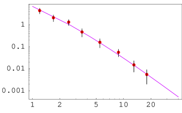
Figure 1: Cross-section $d\sigma/dQ^{2}[pb/GeV^{2}]$ as a function of $Q^{2}$ . The theoretical cross-section is plotted for the best fitted parameters which are $C_{1}=1.0\,{\rm GeV}^{2}$ , $\langle W_{1}\rangle=2.9\,{\rm GeV}$ and $\langle W_{2}\rangle=1.2\,{\rm GeV}$. Experimental data L3Coll come from LEP1 and LEP2 runs.

VII Conclusion

Data thus are in full agreement with the theoretical expectation on the $Q^{2}$ behaviour of the cross section. Because of that the effective structure function $F_{(+,+)}$ is independent of $Q^{2}$ up to the logarithms, as it was said before, our analysis of the data is a direct proof of the relevance of the partonic description of the process $\gamma\gamma^{*}\to\rho^{0}\rho^{0}$ in the kinematics of the L3 experiment.

Much more can be done if detailed experimental results are collected. For instance the angular dependence of the final state is a good test of the validity of the asymptotic form of the generalized distribution amplitudes. The spin structure of the final state, if elucidated, would allow to disentangle the roles of the nine generalized distribution amplitudes. The $W^{2}$ behaviour of the cross section may have some interesting features. It depends much on the possible resonances which are able to couple to two $\rho$ mesons. Its Fourier transform allows to have access to an impact picture of exclusive fragmentation PS . The $\rho^{+}\rho^{-}$ channel may be calculated along the same lines. In that case a brehmstrahlung subprocess where the mesons are radiated from the lepton line must be added. The charge and spin asymmetries then come from the interference of the two processes. In that way one may also study the large contribution of $4\pi$ continuum. These items will be discussed in a forthcoming publication.

We acknowledge useful discussions and correspondance with M. Diehl, A. Nesterenko and I. Vorobiev.This work has been supported in part by RFFI Grant 03-02-16816 and by INTAS Grant (Project 587, call 2000).

References

- (1) H. Terazawa, Rev. Mod. Phys. 45 (1973) 615.
- (2) V.M. Budnev et al., Phys. Rept. 15C (1975) 181.
-
(3)
S.J. Brodsky, hep-ph/9708345, talk presented at
PHOTON 97, Egmond aan Zee, Netherlands, May 1997;
M.R. Pennington, Nucl. Phys. B (Proc. Suppl.) 82 (2000) 291 [hep-ph/9907353]. -
(4)
M. Diehl, T. Gousset, B. Pire and O.V. Teryaev, Phys. Rev. Lett. 81 (1998) 1782 [hep-ph/9805380];
M. Diehl, T. Gousset and B. Pire, Nucl. Phys. B (Proc. Suppl.) 82 (2000) 322 [hep-ph/9907453]. - (5) D. Mueller et al., Fortschr. Phys. 42 (1994) 101 [hep-ph/9812448].
- (6) A. Freund, Phys. Rev. D61 (2000) 074010 [hep-ph/9903489].
- (7) G.P. Lepage and S.J. Brodsky, Phys. Rev. D22 (1980) 2157.
- (8) L3 Collaboration, talk presented by S. Nesterov in ”PHOTON 03” Workshop, April, 7-11 2003, Frascati, Italy (these proceedings)
- (9) M. Diehl, T. Gousset and B. Pire, Phys. Rev. D 62 (2000) 073014
- (10) E. R. Berger, F. Cano, M. Diehl and B. Pire, Phys. Rev. Lett. 87 (2001) 142302
- (11) I. V. Anikin and O. V. Teryaev, Phys. Lett. B 509 (2001) 95.
- (12) S. L. Meyer, ”Data analysis for scientists and engineers”, Wiley series in probability and mathematical statistics, Edt. R. A. Bradley and J. S. Hunter, (1975)
- (13) M. V. Polyakov, Nucl. Phys. B 555 (1999) 231 [hep-ph/9809483].
- (14) B. Pire and L. Szymanowski, Phys. Lett. B 556 (2003) 129 [hep-ph/0212296].