Study of $\tilde{t}$ and $\tilde{b}$ at LHC

Abstract

In supersymmetric models a gluino can decay into $tb\tilde{\chi}^{\pm}_{1}$ through a stop or a sbottom. The decay chain produces an edge structure in the $m_{tb}$ distribution. Monte Carlo simulation studies show that the end point and the edge height would be measured at the CERN LHC by using a sideband subtraction technique. The stop and sbottom masses as well as their decay branching ratios are constrained by the measurement. We study interpretations of the measurement.

The minimal supersymmetric standard model (MSSM) is one of the promising extensions of the standard model. The model requires superpartners of the standard model particles (sparticles), and the large hadron collider (LHC) at CERN might confirm the existence of the new particles  [?]. Among the sparticles the third generation squarks, stops ($\tilde{t}_{i}$) and sbottoms ($\tilde{b}_{i}$) ($i=1,2$), get special imprints from physics at the very high energy scale. Even is the scalar masses are universal at a high energy scale, the third generation squarks are much lighter than the first and second generation squarks due to the Yukawa running effect. On the other hand, some SUSY breaking models have non-universal boundary conditions for the third generation mass parameters at the GUT scale. Measurement of the sparticle masses provides a way to probe the origin of the SUSY breaking in nature.

At the LHC, we may be able to access the nature of the stop and sbottom provided that they are lighter than the gluino ($\tilde{g}$). In that case, they copiously arise from the gluino decay. The relevant decay modes for $\tilde{b}_{i}$ ($i=1,2$), $\tilde{t}_{1}$, to charginos $\tilde{\chi}_{j}^{\pm}$ ($j=1,2$) or neutralinos $\tilde{\chi}^{0}_{j}$ ($j=1,2,3,4$) are (indices to distinguish a particle and its anti-particle is suppressed unless otherwise stated), ${\rm(I)}_{j}~{}{\tilde{g}}\rightarrow b{\tilde{b}_{1}}\rightarrow bb\tilde{\chi}^{0}_{j}\ (\rightarrow bbl^{+}l^{-}\tilde{\chi}^{0}_{1})$, ${\rm(II)}_{j}~{}{\tilde{g}}\rightarrow t{\tilde{t}_{1}}\rightarrow tt\tilde{\chi}^{0}_{j}$, ${\rm(III)}_{j}~{}{\tilde{g}}\rightarrow t{\tilde{t}_{1}}\rightarrow tb\tilde{\chi}^{\pm}_{j}$, ${\rm(III)}_{ij}~{}{\tilde{g}}\rightarrow b\tilde{b}_{i}\rightarrow bW{\tilde{t}_{1}}\rightarrow bbW\tilde{\chi}^{\pm}_{j}$, ${\rm(IV)}_{ij}~{}{\tilde{g}}\rightarrow b\tilde{b}_{i}\rightarrow tb\tilde{\chi}^{\pm}_{j}$. In previous literatures  [?,?], the lighter sbottom $\tilde{b}_{1}$ is often studied through the mode (I)₂, namely the $bb\tilde{\chi}^{0}_{2}\rightarrow bbl^{+}l^{-}\tilde{\chi}^{0}_{1}$ channel. This mode is important when the second lightest neutralino $\tilde{\chi}^{0}_{2}$ has substantial branching ratios into leptons.

Recently we proposed to measure the edge position of the $m_{tb}$ distribution for the modes (III)₁ and (IV)₁₁, where $m_{tb}$ is the invariant mass of a top-bottom ($tb$) system [?,?]. We focused on the reconstruction of hadronic decays of the top quark, because the $m_{tb}$ distribution of the decay makes a clear “edge” in this case. The parton level $m_{tb}$ distributions for the modes (III)_j and (IV)_ij are expressed as functions of $m_{\tilde{g}}$, $m_{\tilde{t}_{1}}$, $m_{\tilde{b}_{i}}$, and the chargino mass $m_{\tilde{\chi}_{j}^{\pm}}$: $d\Gamma/dm_{tb}\propto m_{tb}$.

The events containing $tb$ are selected by requiring the following condition in addition to the standard SUSY cuts: 1) Two and only two $b$ jets. 2) Jet pairs consistent with a hadronic $W$ boson decay, $|m_{jj}-m_{W}|<15$ GeV. 3) The invariant mass of the jet pair and one of the $b$-jets, $m_{bjj}$, satisfies $|m_{bjj}-m_{t}|<30$ GeV. The events after the selection contain misreconstructed events. We use a $W$ sideband method to estimate the background distribution due to misreconstructed events. Monte Carlo simulations show that the distribution of the signal modes (III) and (IV) after subtracting the background is very close to the parton level distribution. The distribution is then fitted by a simple fitting function described with the end point $M_{tb}^{\rm fit}$, the edge height $h$ per $\Delta m$ bin, and a smearing parameter.

The edge position (end point) of the $m_{tb}$ distribution $M_{tb}$ for the modes (III)₁ and (IV)₁₁ are sometimes very close. When they are experimentally indistinguishable, it is convenient to define a weighted mean of the end points;

$$M_{tb}^{\rm w}=\frac{{\rm Br}({\rm III})M_{tb}({\rm III})_{1}+{\rm Br}({\rm IV})_{11}M_{tb}({\rm IV})_{11}}{{\rm Br}({\rm III})+{\rm Br}({\rm IV})_{11}},$$ (1)

where ${\rm Br}({\rm III})\equiv{\rm Br}({\rm III})_{1}+{\rm Br}({\rm III})_{11}+{\rm Br}({\rm III})_{21}$.

         

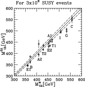
Figure  1.: Left:Relation between $M^{\rm w}_{tb}$ and $M^{\rm fit}_{tb}$ for the sample points. The solid line corresponds to $M^{\rm w}_{tb}=M^{\rm fit}_{tb}$. Bars with a diamond and a circle correspond to PYTHIA and HERWIG samples, respectively. Right: Relation between $N_{\rm edge}/N_{\rm all}$ and ${\rm Br(edge)}/{\rm Br}(\tilde{g}\rightarrow bbX)$.

The relation between $M_{tb}^{\rm w}$ and $M_{tb}^{\rm fit}$ for several model points are shown in Fig. 1 (left). Here we generated $3\times 10^{6}$ SUSY events for each model point. The fitted value $M_{tb}^{\rm fit}$ increases linearly with the weighted end point $M_{tb}^{\rm w}$. The fitted value $M_{tb}^{\rm fit}$ tends to be lower than $M_{tb}^{\rm w}$, which is the effect of particle missed outside the jet cones.

We now discuss the relation between the edge height $h$ and the number of reconstructed $tb$ events. The number of the reconstructed “edge” events $N_{\rm edge}$ arising from the decay chains (III) and (IV) may be estimated from $M_{tb}^{\rm fit}$, $h$ per the bin size $\Delta m$ as follows,

$$N_{\rm edge}\sim N_{\rm fit}=\frac{h}{2}\left(\frac{m_{t}}{M^{\rm fit}_{tb}}+1\right)\times\frac{M^{\rm fit}_{tb}-m_{t}}{\Delta m}.$$ (2)

This formula is obtained by assuming the parton level distribution. The consistency between $N_{\rm edge}\sim N_{\rm fit}$ is checked by using the generator information in Ref.  [?].

In the MSUGRA model, the decay modes which involve $W$ bosons (modes (II), (III) and (IV)) often dominate the gluino decays to $bbX$. In that case the numbers of events are given approximately as

$$N_{\rm fit} \sim {\epsilon_{tb}}{\rm Br(edge)}\left[2N(\tilde{g}\tilde{g})\left(1-{\rm Br}(\tilde{g}\rightarrow bbX)\right)+N(\tilde{g}\tilde{q})+N(\tilde{g}\tilde{q}^{*})\right],$$ (3)

$$N_{\rm all} \sim {\epsilon_{tb}}{\rm Br}(\tilde{g}\rightarrow bbX)\left[2N(\tilde{g}\tilde{g})\left(1-{\rm Br}(\tilde{g}\rightarrow bbX)\right)+N(\tilde{g}\tilde{q})+N(\tilde{g}\tilde{q}^{*})\right],$$ (4)

where ${\rm Br(edge)}\equiv\rm Br(III)_{1}+Br(III)_{11}+Br(III)_{21}+Br(IV)_{11}$ and ${\rm Br}(\tilde{g}\to bbX)$ is the branching ratio of the gluino decaying into stop or sbottom, thus having two bottom quarks in the final state. Therefore ${\rm Br(edge)}$ $/{\rm Br}(\tilde{g}\rightarrow bbX)\sim N_{\rm fit}/N_{\rm all}$ is expected.

In Fig. 1(right), we plot the ratio $N_{\rm edge}/N_{\rm all}$ as a function of ${\rm Br(edge)}$ $/{\rm Br}(\tilde{g}\rightarrow bbX)$. The points tend to be on the expected line $N_{\rm edge}/N_{\rm all}={\rm Br(edge)}/{\rm Br}(\tilde{g}\rightarrow bbX)$. Some points in the plots are away from the line: The point “C” is off because the chargino has large branching ratios into leptons. At the point “T1”, the stop mass is significantly light and $\tilde{t}_{1}\tilde{t}^{*}_{1}$ productions contributes to $N_{\rm all}$. The points “E1” and “E2” are significantly off because the first and the second generation squarks dominantly decay into the gluino, and the events containing two bottom quarks are not dominant. . These exceptional cases will be easily distinguished by looking into the data from LHC or a proposed O(1)TeV linear collider.

The $M_{tb}^{\rm fit}$ contains information on $\tilde{t}_{1}$ as can be seen in Eq.(1). However, the definition also depends on the electroweak SUSY parameters and the SUSY parameters in the sbottom sector. Some model assumptions or inputs from the other measurements are necessary. In MSUGRA, the $M_{tb}$ and $h$ measurement constrain the trilinear coupling at GUT scale $A_{0}$. $\Delta A_{0}\sim 50$ GeV for $m_{\tilde{g}}\sim m_{\tilde{q}}\sim 700$ GeV are found. On the other hand, if a $e^{+}e^{-}$ collider at O(1TeV) is built, the measurements of the sparticle productions at the LC would constrain the electroweak SUSY parameters precisely. In that case the sbottom and stop studies at LHC would be significantly improved so that stop and sbottom masses and their mixing angle are measured  [?].

Acknowledgment: I thank J. Hisano and K. Kawawagoe for collaboration, and the ATLAS collaboration members for useful discussion. We have made use of the physics analysis framework and tools which are the result of collaboration-wide efforts. This work is supported in part by the Grant-in-Aid for Science Research, Ministry of Education, Science and Culture, Japan (No.13135297 and No.14046225 for JH, No.11207101 for KK, and No.14540260 and 14046210 for MMN).

REFERENCES

- [1] ATLAS: Detector and physics performance technical design report, CERN-LHCC-99-14.
- [2] I. Hinchliffe, F. E. Paige, M. D. Shapiro, J. Soderqvist and W. Yao, Phys. Rev. D 55, 5520 (1997).
- [3] J. Hisano, K. Kawagoe, R. Kitano and M. M. Nojiri, Phys. Rev. D 66, 115004 (2002).
- [4] J. Hisano, K. Kawagoe and M. M. Nojiri, arXiv:hep-ph/0304214.
- [5] J. Hisano, J. Kalinowski, K. Kawagoe, Gudrid Moortgat-Pick, Mihoko M. Nojiri and Giacomo Polesello, a contribution to the LHC/LC study. http://www.ippp.dur.ac.uk/~georg/lhclc.