WMAPping inflationary physics

Abstract

We extract parameters relevant for distinguishing among single-field inflation models from the Wilkinson Microwave Anisotropy Probe (WMAP) data set, and from a combination of the WMAP data and seven other Cosmic Microwave Background (CMB) experiments. We use only CMB data and perform a likelihood analysis over a grid of models including the full error covariance matrix. We find that a model with a scale-invariant scalar power spectrum ($n=1$), no tensor contribution, and no running of the spectral index, is within the 1-$\sigma$ contours of both data sets. We then apply the Monte Carlo reconstruction technique to both data sets to generate an ensemble of inflationary potentials consistent with observations. None of the three basic classes of inflation models (small-field, large-field, and hybrid) are completely ruled out, although hybrid models are favored by the best-fit region. The reconstruction process indicates that a wide variety of smooth potentials for the inflaton are consistent with the data, implying that the first-year WMAP result is still too crude to constrain significantly either the height or the shape of the inflaton potential. In particular, the lack of evidence for tensor fluctuations makes it impossible to constrain the energy scale of inflation. Nonetheless, the data rule out a large portion of the available parameter space for inflation. For instance, we find that potentials of the form $V=\lambda\phi^{4}$ are ruled out to $3\sigma$ by the combined data set, but not by the WMAP data taken alone.

I Introduction

One of the fundamental ideas of modern cosmology is that there was an epoch early in the history of the universe when potential, or vacuum, energy dominated other forms of energy densities such as matter or radiation. During such a vacuum-dominated era the scale factor grew exponentially (or nearly exponentially) in some small time. During this phase, dubbed inflation guth81 ; lrreview , a small, smooth spatial region of size of order the Hubble radius grew so large that it easily could encompass the comoving volume of the entire presently observable universe. If the universe underwent such a period of rapid expansion, one can understand why the observed universe is homogeneous and isotropic to such high accuracy.

One of the predictions of the simplest models of inflation is a spatially flat Universe, i.e., $\Omega_{tot}=1$, with great precision. Inflation has also become the dominant paradigm for understanding the initial conditions for structure formation and for Cosmic Microwave Background (CMB) anisotropy. In the inflationary picture, primordial density and gravity-wave (tensor) fluctuations are created from quantum fluctuations and “redshifted” out of the horizon during an early period of superluminal expansion of the universe, where they are “frozen” as perturbations in the background metric muk81 ; hawking82 ; starobinsky82 ; guth82 ; bardeen83 . Metric perturbations at the surface of last scattering are observable as temperature anisotropies in the CMB. The first and most impressive confirmation of the inflationary paradigm came when the CMB anisotropies were detected by the Cosmic Background Explorer (COBE) satellite in 1992 smoot92 ; bennett96 ; gorski96 . Subsequently, it became clear that the measurements of the spectrum of the CMB anisotropy can provide very detailed information about fundamental cosmological parameters cp and other crucial parameters for particle physics.

In the past few years, a number of balloon-borne and terrestrial experiments have mapped out the CMB angular anisotropies toco ; b97 ; Netterfield ; halverson ; cbi ; vsa ; benoit , revealing a remarkable agreement between the data and the inflationary predictions of a flat universe with a nearly scale-invariant spectrum of adiabatic primordial density perturbations, (see e.g., debe2001 ; pryke ; stompor ; wang ; cbit ; vsat ; saralewis ; mesilk ; caro ).

Despite the simplicity of the inflationary paradigm, the number of inflation models that have been proposed in the literature is enormous lrreview . This is true even if we limit ourselves to models with only one scalar field (the inflaton). With the previous data on CMB anisotropies from balloon and terrestrial experiments it has been possible for the first time to place interesting constraints on the space of possible inflation models dodelson97 ; kinney98a ; probes . However, the quality of the data were not good enough to rule out entire classes of models. A boost along these lines has been very recently provided by the data of the Wilkinson Microwave Anisotropy Probe (WMAP) mission, which has marked the beginning of the precision era of the CMB measurements in space wmap1 ; kogutt . The WMAP collaboration has produced a full-sky map of the angular variations in the microwave flux, in particular the cosmic microwave background, with unprecedented accuracy. WMAP data support the inflationary mechanism for the generation of curvature superhorizon fluctuations and provide a strong bound on the possible admixture of isocurvature modes wmapinf . Furthermore, consistent with the simplest single-field models of inflation nong , no evidence of nongaussianity is found wmapnong .

The goal of this paper is to use the WMAP data to discriminate among the various single-field inflationary models. To obtain some indication of the robustness of our analysis, we also consider a data set consisting of WMAP augmented with several other CMB experiments. For single-field inflation models, the relevant parameter space for distinguishing among models is defined by the scalar spectral index $n$, the ratio of tensor to scalar fluctuations $r$, and the running of the scalar spectral index $dn/d\ln{k}$. We employ Monte Carlo reconstruction, a stochastic method for “inverting” observational constraints to determine an ensemble of inflationary potentials compatible with observation kinney02 ; easther02 . In addition to encompassing a broader set of models than usually considered (large-field, small-field, hybrid and linear models), Monte Carlo reconstruction makes it possible easily to incorporate constraints on the running of the spectral index as well as to include effects to higher order in slow roll.

Since studies on the implications of WMAP data for inflation wmapinf ; barger have already appeared, we briefly mention the different elements between our analysis and others. (We will elaborate on these differences later.) The WMAP collaboration analysis wmapinf included WMAP data, additional CMB data (CBI cbi and ACBAR acbar ), large-scale structure data (2dFGRS 2df ), as well as Lyman-$\alpha$ power spectrum data lyman . They used a Markov Chain Monte Carlo technique to explore the likelihood surface. Barger et al. barger , considered WMAP data only, but with a top-hat prior on the Hubble constant $h$ ($H_{0}=$ 100 $h$ km sec^-1 Mpc^-1) from the HST key project hst . Also, Barger et al. did not consider a running of the scalar spectral index. We only consider CMB data. We first analyze just the WMAP results. We then analyze the WMAP data set in conjunction with other CMB data sets (BOOMERanG-98 ruhl , MAXIMA-1 lee , DASI halverson , CBI cbi , ACBAR acbar , VSAE grainge , and Archeops benoit ). We employ a grid of models in the likelihood analysis, which differs from the method used by the WMAP team.

The paper is organized as follows. In Sec. II we discuss single-field inflation and the relevant observables in more detail. In Sec. III we discuss the inflationary model space, and in Sec. IV we describe the Monte Carlo reconstruction technique. Section V describes the methods used for the CMB analysis. In Sec. VI we present the constraints from the CMB anisotropy data sets. In Sec. VII we present our conclusions.

II Single-field inflation and the inflationary observables

In this section we briefly review scalar field models of inflationary cosmology, and explain how we relate model parameters to observable quantities. Inflation, in its most general sense, can be defined to be a period of accelerating cosmological expansion during which the universe evolves toward homogeneity and flatness. This acceleration is typically a result of the universe being dominated by vacuum energy, with an equation of state $p\simeq-\rho$. Within this broad framework, many specific models for inflation have been proposed. We limit ourselves here to models with “normal” gravity (i.e., general relativity) and a single order parameter for the vacuum, described by a slowly rolling scalar field $\phi$, the inflaton. These assumptions are not overly restrictive; the most widely studied inflation models fall within this category, including Linde’s “chaotic” inflation scenario linde83 , inflation from pseudo Nambu-Goldstone bosons (“natural” inflation freese90 ), dilaton-like models involving exponential potentials (power-law inflation), hybrid inflation linde91 ; linde94 ; copeland94 , and so forth. Other models, such as Starobinsky’s $R^{2}$ model starobinsky80 and versions of extended inflation, can, through a suitable transformation, be viewed in terms of equivalent single-field models. Of course in single-field models of inflation, the inflaton “field” need not be a fundamental field at all. Also, some “single-field” models require auxiliary fields. Hybrid inflation models linde91 ; linde94 ; copeland94 , for example, require a second field to end inflation. What is significant is that the inflationary epoch be described by a single dynamical order parameter, the inflaton field.

A scalar field in a cosmological background evolves with an equation of motion

$$\ddot{\phi}+3H\dot{\phi}+V^{\prime}\left(\phi\right)=0.$$ (1)

The evolution of the scale factor is given by the scalar field dominated FRW equation,

$$H^{2} ={8\pi\over 3m_{\rm Pl}^{2}}\left[{1\over 2}\dot{\phi}^{2}+V\left(\phi\right)\right],$$ (2)

$$\left(\ddot{a}\over a\right) ={8\pi\over 3m_{\rm Pl}^{2}}\left[V\left(\phi\right)-\dot{\phi}^{2}\right].$$ (3)

Here $m_{\rm Pl}=G^{-1/2}\simeq 10^{19}\ {\rm GeV}$ is the Planck mass, and we have assumed a flat Friedmann-Robertson-Walker metric,

$$g_{\mu\nu}={\rm diag}(1,-a^{2},-a^{2}-a^{2}),$$ (4)

where $a^{2}(t)$ is the scale factor of the universe. Inflation is defined to be a period of accelerated expansion, $\ddot{a}>0$. A powerful way of describing the dynamics of a scalar field-dominated cosmology is to express the Hubble parameter as a function of the field $\phi$, $H=H(\phi)$, which is consistent provided $\phi$ is monotonic in time. The equations of motion become grishchuk88 ; muslimov90 ; salopek90 ; lidsey95 :

$$\dot{\phi}=-{m_{\rm Pl}^{2}\over 4\pi}H^{\prime}(\phi),$$ (5)

$$\left[H^{\prime}(\phi)\right]^{2}-{12\pi\over m_{\rm Pl}^{2}}H^{2}(\phi)=-{32\pi^{2}\over m_{\rm Pl}^{4}}V(\phi).$$ (6)

These are completely equivalent to the second-order equation of motion in Eq. (1). The second of the above equations is referred to as the Hamilton-Jacobi equation, and can be written in the useful form

$$H^{2}(\phi)\left[1-{1\over 3}\epsilon(\phi)\right]=\left({8\pi\over 3m_{\rm Pl}^{2}}\right)V(\phi),$$ (7)

where $\epsilon$ is defined to be

$$\epsilon\equiv{m_{\rm Pl}^{2}\over 4\pi}\left({H^{\prime}(\phi)\over H(\phi)}\right)^{2}.$$ (8)

The physical meaning of $\epsilon$ can be seen by expressing Eq. (3) as

$$\left({\ddot{a}\over a}\right)=H^{2}(\phi)\left[1-\epsilon(\phi)\right],$$ (9)

so that the condition for inflation $(\ddot{a}/a)>0$ is given by $\epsilon<1$. The scale factor is given by

$$a\propto e^{N}=\exp\left[\int_{t_{0}}^{t}{H\,dt}\right],$$ (10)

where the number of e-folds $N$ is

$$N\equiv\int_{t}^{t_{e}}{H\,dt}=\int_{\phi}^{\phi_{e}}{{H\over\dot{\phi}}\,d\phi}={2\sqrt{\pi}\over m_{\rm Pl}}\int_{\phi_{e}}^{\phi}{d\phi\over\sqrt{\epsilon(\phi)}}.$$ (11)

To create the observed flatness and homogeneity of the universe, we require many e-folds of inflation, typically $N\simeq 60$. This figure varies somewhat with the details of the model. We can relate a comoving scale $k$ in the universe today to the number of e-folds $N$ before the end of inflation by lidsey97

$$N(k)=62-\ln\frac{k}{a_{0}H_{0}}-\ln\frac{10^{16}{\rm GeV}}{V_{k}^{1/4}}+\ln\frac{V_{k}^{1/4}}{V_{e}^{1/4}}-\frac{1}{3}\ln\frac{{V_{e}}^{1/4}}{\rho_{{\rm RH}}^{1/4}}\,.$$ (12)

Here $V_{k}$ is the potential when the mode leaves the horizon, $V_{e}$ is the potential at the end of inflation, and $\rho_{{\rm RH}}$ is the energy density after reheating. Scales of order the current horizon size exited the horizon at $N\left(k\right)\sim 60$. Since this number depends, for example, on the details of reheating, we will allow $N$ to vary within the range $40\leq N\leq 70$ for any given model in order to consider the most general case. (Dodelson and Hui have recently argued that the value of $N$ corresponding to the current horizon size can be no larger than 60 dodelson03 , so in this sense we are being more general than is necessary.)

We will frequently work within the context of the slow roll approximation linde82 ; albrecht82 , which is the assumption that the evolution of the field is dominated by drag from the cosmological expansion, so that $\ddot{\phi}\simeq 0$ and

$$\dot{\phi}\simeq-{V^{\prime}\over 3H}.$$ (13)

The equation of state of the scalar field is dominated by the potential, so that $p\simeq-\rho$, and the expansion rate is approximately

$$H\simeq\sqrt{{8\pi\over 3m_{\rm Pl}^{2}}V\left(\phi\right)}.$$ (14)

The slow roll approximation is consistent if both the slope and curvature of the potential are small, $V^{\prime},\ V^{\prime\prime}\ll V$. In this case the parameter $\epsilon$ can be expressed in terms of the potential as

$$\epsilon\equiv{m_{\rm Pl}^{2}\over 4\pi}\left({H^{\prime}\left(\phi\right)\over H\left(\phi\right)}\right)^{2}\simeq{m_{\rm Pl}^{2}\over 16\pi}\left({V^{\prime}\left(\phi\right)\over V\left(\phi\right)}\right)^{2}.$$ (15)

We will also define a second “slow roll parameter” $\eta$ by:

$$\eta\left(\phi\right) \equiv {m_{\rm Pl}^{2}\over 4\pi}\left({H^{\prime\prime}\left(\phi\right)\over H\left(\phi\right)}\right)$$ (16)

$$\simeq {m_{\rm Pl}^{2}\over 8\pi}\left[{V^{\prime\prime}\left(\phi\right)\over V\left(\phi\right)}-{1\over 2}\left({V^{\prime}\left(\phi\right)\over V\left(\phi\right)}\right)^{2}\right].$$ (17)

Slow roll is then a consistent approximation for $\epsilon,\ \eta\ll 1$.

Inflation models not only explain the large-scale homogeneity of the universe, but also provide a mechanism for explaining the observed level of inhomogeneity as well. During inflation, quantum fluctuations on small scales are quickly redshifted to scales much larger than the horizon size, where they are “frozen” as perturbations in the background metric muk81 ; hawking82 ; starobinsky82 ; guth82 ; bardeen83 . The metric perturbations created during inflation are of two types: scalar, or curvature perturbations, which couple to the stress-energy of matter in the universe and form the “seeds” for structure formation, and tensor, or gravitational wave perturbations, which do not couple to matter. Both scalar and tensor perturbations contribute to CMB anisotropy. Scalar fluctuations can also be interpreted as fluctuations in the density of the matter in the universe. Scalar fluctuations can be quantitatively characterized by perturbations $P_{\cal R}$ in the intrinsic curvature scalar. As long as the equation of state $\epsilon$ is slowly varying, the curvature perturbation can be shown to be mukhanov85 ; mukhanov88 ; mukhanov92 ; stewart93

$$P_{\cal R}^{1/2}\left(k\right)=\frac{1}{2\pi}\left[{H\over m_{\rm Pl}}{1\over\sqrt{\epsilon}}\right]_{k=aH}.$$ (18)

The fluctuation power spectrum is in general a function of wavenumber $k$, and is evaluated when a given mode crosses outside the horizon during inflation, $k=aH$. Outside the horizon, modes do not evolve, so the amplitude of the mode when it crosses back inside the horizon during a later radiation- or matter-dominated epoch is just its value when it left the horizon during inflation.

The spectral index $n$ for $P_{\cal R}$ is defined by

$$n-1\equiv{d\ln P_{\cal R}\over d\ln k},$$ (19)

so that a scale-invariant spectrum, in which modes have constant amplitude at horizon crossing, is characterized by $n=1$. Some inflation models predict running of the spectral index with scale stewart97 ; linde97 ; stewart97a ; copeland97 ; kinney97 ; covi98 ; kinney98 ; covi99 ; covi00 or even sharp features in the power spectrum featuresinpowerspectrum . We will consider the running of the spectral index in more detail on Sec. IV.

Instead of specifying the fluctuation amplitude directly as a function of $k$, it is often convenient to specify it as a function of the number of e-folds $N$ before the end of inflation at which a mode crossed outside the horizon. Scales of interest for current measurements of CMB anisotropy crossed outside the horizon at $N\sim 60$, so that $P_{\cal R}$ is conventionally evaluated at $P_{\cal R}\left({N\sim 60}\right)$.

The power spectrum of tensor fluctuation modes is given by starobinsky79 ; rubakov82 ; fabbri83 ; abbot84 ; starobinsky85

$$P_{T}^{1/2}\left(k_{N}\right)={1\over 2\pi}\left[\frac{H}{m_{\rm Pl}}\right]_{N}.$$ (20)

The ratio of tensor to scalar modes is then

$${P_{T}\over P_{\cal R}}=\epsilon,$$ (21)

so that tensor modes are negligible for $\epsilon\ll 1$. Tensor and scalar modes both contribute to CMB temperature anisotropy. If the contribution of tensor modes to the CMB anisotropy can be neglected, normalization to the COBE four-year data gives bunn96 ; lyth96 $P_{\cal R}^{1/2}=4.8\times 10^{-5}$. In the next section, we will describe the predictions of various models in this parameter space.

III The inflationary model space

To summarize the results of the previous section, inflation generates scalar (density) and tensor (gravity wave) fluctuations which are generally well approximated by power laws:

$$P_{\cal R}\left(k\right)\propto k^{n-1};\qquad P_{T}\left(k\right)\propto k^{n_{T}}.$$ (22)

In the limit of slow roll, the spectral indices $n$ and $n_{T}$ vary slowly or not at all with scale. We can write the spectral indices $n$ and $n_{T}$ to lowest order in terms of the slow roll parameters $\epsilon$ and $\eta$ as stewart93 :

$$n\simeq 1-4\epsilon+2\eta,$$ (23)

$$n_{T}\simeq -2\epsilon.$$ (24)

The tensor spectral index is not an independent parameter, but is proportional to the tensor/scalar ratio, given to lowest order in slow roll by

$$n_{T}\simeq-2\epsilon=-2{P_{T}\over P_{\cal R}}.$$ (25)

This is known as the consistency relation for inflation. (This relation holds only for single-field inflation, and weakens to an inequality for inflation involving multiple degrees of freedom polarski95 ; bellido95 ; sasaki96 .) A given inflation model can therefore be described to lowest order in slow roll by three independent parameters, $P_{\cal R}$, $P_{T}$, and $n$. If we wish to include higher-order effects, we have a fourth parameter describing the running of the scalar spectral index, $dn/d\ln{k}$.

The tensor/scalar ratio is frequently expressed as a ratio of their contributions to the CMB quadrupole,

$$r\equiv{C^{\rm Tensor}_{2}\over C^{\rm Scalar}_{2}}.$$ (26)

The relation between $r$ and ratio of amplitudes in the primordial power spectra $P_{T}/P_{\cal R}$ depends on the background cosmology, in particular the densities of matter ($\Omega_{\rm m}$) and cosmological constant ($\Omega_{\Lambda}$). For the currently favored values of $\Omega_{\rm m}\simeq 0.3$ and $\Omega_{\Lambda}\simeq 0.7$, the relation is approximately

$$r\simeq 10\epsilon,$$ (27)

to lowest order in slow roll. Conventions for the normalization of this parameter vary widely in the literature. In particular, Peiris et al. wmapinf use $r\simeq 16\epsilon$.

Calculating the CMB fluctuations from a particular inflationary model reduces to the following basic steps: (1) from the potential, calculate $\epsilon$ and $\eta$. (2) From $\epsilon$, calculate $N$ as a function of the field $\phi$. (3) Invert $N\left(\phi\right)$ to find $\phi_{N}$. (4) Calculate $P_{\cal R}$, $n$, and $P_{T}$ as functions of $\phi$, and evaluate them at $\phi=\phi_{N}$. For the remainder of the paper, all parameters are assumed to be evaluated at $\phi=\phi_{N}$.

Even restricting ourselves to a simple single-field inflation scenario, the number of models available to choose from is large lrreview . It is convenient to define a general classification scheme, or “zoology” for models of inflation. We divide models into three general types: large-field, small-field, and hybrid, with a fourth classification, linear models, serving as a boundary between large- and small-field. A generic single-field potential can be characterized by two independent mass scales: a “height” $\Lambda^{4}$, corresponding to the vacuum energy density during inflation, and a “width” $\mu$, corresponding to the change in the field value $\Delta\phi$ during inflation:

$$V\left(\phi\right)=\Lambda^{4}f\left({\phi\over\mu}\right).$$ (28)

Different models have different forms for the function $f$. The height $\Lambda$ is fixed by normalization, so the only free parameter is the width $\mu$.

With the normalization fixed, the relevant parameter space for distinguishing between inflation models to lowest order in slow roll is then the $r\,-\,n$ plane. (To next order in slow-roll parameters, one must introduce the running of $n$.) Different classes of models are distinguished by the value of the second derivative of the potential, or, equivalently, by the relationship between the values of the slow-roll parameters $\epsilon$ and $\eta$. Each class of models has a different relationship between $r$ and $n$. For a more detailed discussion of these relations, the reader is referred to Refs. dodelson97 ; kinney98a .

First order in $\epsilon$ and $\eta$ is sufficiently accurate for the purposes of this Section, and for the remainder of this Section we will only work to first order. The generalization to higher order in slow roll will be discussed in Sec. IV.

III.1 Large-field models: $-\epsilon<\eta\leq\epsilon$

Large-field models have inflaton potentials typical of “chaotic” inflation scenarios linde83 , in which the scalar field is displaced from the minimum of the potential by an amount usually of order the Planck mass. Such models are characterized by $V^{\prime\prime}\left(\phi\right)>0$, and $-\epsilon<\eta\leq\epsilon$. The generic large-field potentials we consider are polynomial potentials $V\left(\phi\right)=\Lambda^{4}\left({\phi/\mu}\right)^{p}$, and exponential potentials, $V\left(\phi\right)=\Lambda^{4}\exp\left({\phi/\mu}\right)$. For the case of an exponential potential, $V\left(\phi\right)\propto\exp\left({\phi/\mu}\right)$, the tensor/scalar ratio $r$ is simply related to the spectral index as

$$r=5\left(1-n\right).$$ (29)

This result is often incorrectly generalized to all slow-roll models, but is in fact characteristic only of power-law inflation. For inflation with a polynomial potential, $V\left(\phi\right)\propto\phi^{p}$, we again have $r\propto 1-n$,

$$r=5\left({p\over p+2}\right)\left(1-n\right),$$ (30)

so that tensor modes are large for significantly tilted spectra. We will be particularly interested in models with $p=4$ as a test case for our ability to rule out models. For $p=4$, the observables are given in terms of the number of e-folds $N$ by

$$r = {10\over N+1},$$ (31)

$$1-n = {3\over N+1}.$$ (32)

III.2 Small-field models: $\eta<-\epsilon$

Small-field models are the type of potentials that arise naturally from spontaneous symmetry breaking (such as the original models of “new” inflation linde82 ; albrecht82 ) and from pseudo Nambu-Goldstone modes (natural inflation freese90 ). The field starts from near an unstable equilibrium (taken to be at the origin) and rolls down the potential to a stable minimum. Small-field models are characterized by $V^{\prime\prime}\left(\phi\right)<0$ and $\eta<-\epsilon$. Typically $\epsilon$ (and hence the tensor amplitude) is close to zero in small-field models. The generic small-field potentials we consider are of the form $V\left(\phi\right)=\Lambda^{4}\left[1-\left({\phi/\mu}\right)^{p}\right]$, which can be viewed as a lowest-order Taylor expansion of an arbitrary potential about the origin. The cases $p=2$ and $p>2$ have very different behavior. For $p=2$,

$$r=5(1-n)\exp\left[-1-N\left(1-n\right)\right],$$ (33)

where $N$ is the number of e-folds of inflation. For $p>2$, the scalar spectral index is

$$n\simeq 1-{2\over N}\left({p-1\over p-2}\right),$$ (34)

independent of $r$. Assuming $\mu<m_{\rm Pl}$ results in an upper bound on $r$ of

$$r<5{p\over N\left(p-2\right)}\left({8\pi\over Np\left(p-2\right)}\right)^{p/\left(p-2\right)}.$$ (35)

III.3 Hybrid models: $0<\epsilon<\eta$

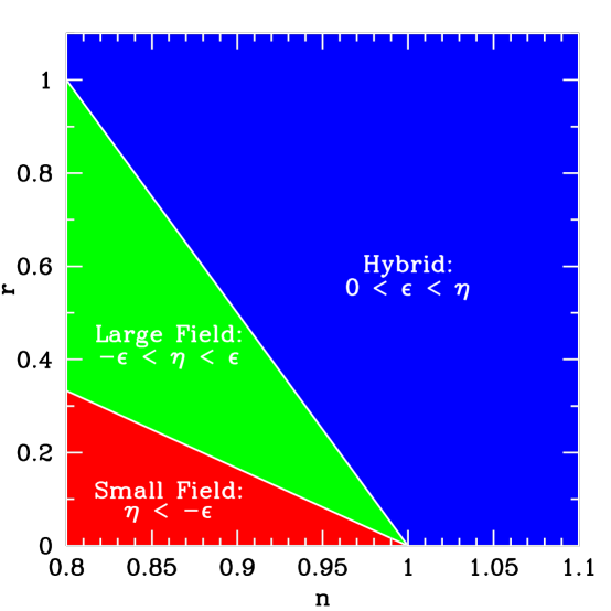
Figure 1: Regions on the $r\,-\,n$ plane. The different types of potentials, small field, large field, and hybrid, occupy different regions of the observable parameter space.

The hybrid scenario linde91 ; linde94 ; copeland94 frequently appears in models which incorporate inflation into supersymmetry. In a typical hybrid inflation model, the scalar field responsible for inflation evolves toward a minimum with nonzero vacuum energy. The end of inflation arises as a result of instability in a second field. Such models are characterized by $V^{\prime\prime}\left(\phi\right)>0$ and $0<\epsilon<\eta$. We consider generic potentials for hybrid inflation of the form $V\left(\phi\right)=\Lambda^{4}\left[1+\left({\phi/\mu}\right)^{p}\right].$ The field value at the end of inflation is determined by some other physics, so there is a second free parameter characterizing the models. Because of this extra freedom, hybrid models fill a broad region in the $r\,-\,n$ plane (see Fig. 1). There is, however, no overlap in the $r\,-\,n$ plane between hybrid inflation and other models. The distinguishing feature of many hybrid models is a blue scalar spectral index, $n>1$. This corresponds to the case $\eta>2\epsilon$. Hybrid models can also in principle have a red spectrum, $n<1$.

III.4 Linear models: $\eta=-\epsilon$

Linear models, $V\left(\phi\right)\propto\phi$, live on the boundary between large-field and small-field models, with $V^{\prime\prime}\left(\phi\right)=0$ and $\eta=-\epsilon$. The spectral index and tensor/scalar ratio are related as:

$$r={5\over 3}\left(1-n\right).$$ (36)

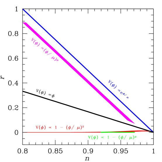
Figure 2: A “zoo plot” of models in the $r\,-\,n$ plane, plotted to first order in slow roll.

This enumeration of models is certainly not exhaustive. There are a number of single-field models that do not fit well into this scheme, for example logarithmic potentials $V\left(\phi\right)\propto\ln\left(\phi\right)$ typical of supersymmetry lrreview . Another example is potentials with negative powers of the scalar field $V\left(\phi\right)\propto\phi^{-p}$ used in intermediate inflation barrow93 and dynamical supersymmetric inflation kinney97 ; kinney98 . Both of these cases require an auxiliary field to end inflation and are more properly categorized as hybrid models, but fall into the small-field region of the $r\,-\,n$ plane. However, the three classes categorized by the relationship between the slow-roll parameters as $-\epsilon<\eta\leq\epsilon$ (large-field), $\eta\leq-\epsilon$ (small-field, linear), and $0<\epsilon<\eta$ (hybrid), cover the entire $r\,-\,n$ plane and are in that sense complete. Figure 1 dodelson97 shows the $r\,-\,n$ plane divided into regions representing the large field, small-field and hybrid cases. Figure 2 shows a “zoo plot” of the particular potentials considered here plotted on the $r\,-\,n$ plane.

IV Monte Carlo reconstruction

In this section we describe Monte Carlo reconstruction, a stochastic method for “inverting” observational constraints to determine an ensemble of inflationary potentials compatible with observation. The method is described in more detail in Refs. kinney02 ; easther02 . In addition to encompassing a broader set of models than we considered in Sec. III, Monte Carlo reconstruction allows us easily to incorporate constraints on the running of the spectral index $dn/d\ln{k}$ as well as to include effects to higher order in slow roll.

We have defined the slow roll parameters $\epsilon$ and $\eta$ in terms of the Hubble parameter $H\left(\phi\right)$ as

$$\epsilon \equiv {m_{\rm Pl}^{2}\over 4\pi}\left({H^{\prime}(\phi)\over H(\phi)}\right)^{2},$$ (37)

$$\eta\left(\phi\right) \equiv {m_{\rm Pl}^{2}\over 4\pi}\left({H^{\prime\prime}\left(\phi\right)\over H\left(\phi\right)}\right).$$ (38)

These parameters are simply related to observables $r\simeq 10\epsilon$, and $n-1\simeq 4\epsilon-2\eta$ to first order in slow roll. (We discuss higher order expressions for the observables below.) Taking higher derivatives of $H$ with respect to the field, we can define an infinite hierarchy of slow roll parameters liddle94 :

$$\sigma \equiv {m_{\rm Pl}\over\pi}\left[{1\over 2}\left({H^{\prime\prime}\over H}\right)-\left({H^{\prime}\over H}\right)^{2}\right],$$ (39)

$${}^{\ell}\lambda_{\rm H} \equiv \left({m_{\rm Pl}^{2}\over 4\pi}\right)^{\ell}{\left(H^{\prime}\right)^{\ell-1}\over H^{\ell}}{d^{(\ell+1)}H\over d\phi^{(\ell+1)}}.$$ (40)

Here we have chosen the parameter $\sigma\equiv 2\eta-4\epsilon\simeq n-1$ to make comparison with observation convenient.

It is convenient to use $N$ as the measure of time during inflation. As above, we take $t_{e}$ and $\phi_{e}$ to be the time and field value at end of inflation. Therefore, $N$ is defined as the number of e-folds before the end of inflation, and increases as one goes backward in time ($dt>0\Rightarrow dN<0$):

$${d\over dN}={d\over d\ln a}={m_{\rm Pl}\over 2\sqrt{\pi}}\sqrt{\epsilon}{d\over d\phi},$$ (41)

where we have chosen the sign convention that $\sqrt{\epsilon}$ has the same sign as $H^{\prime}\left(\phi\right)$:

$$\sqrt{\epsilon}\equiv+{m_{\rm PL}\over 2\sqrt{\pi}}{H^{\prime}\over H}.$$ (42)

Then $\epsilon$ itself can be expressed in terms of $H$ and $N$ simply as,

$${1\over H}{dH\over dN}=\epsilon.$$ (43)

Similarly, the evolution of the higher order parameters during inflation is determined by a set of “flow” equations hoffman00 ; schwarz01 ; kinney02 ,

$${d\epsilon\over dN} = \epsilon\left(\sigma+2\epsilon\right),$$ (44)

$${d\sigma\over dN} = -5\epsilon\sigma-12\epsilon^{2}+2\left({}^{2}\lambda_{\rm H}\right),$$ (45)

$${d\left({}^{\ell}\lambda_{\rm H}\right)\over dN} = \left[\frac{\ell-1}{2}\sigma+\left(\ell-2\right)\epsilon\right]\left({}^{\ell}\lambda_{\rm H}\right)+{}^{\ell+1}\lambda_{\rm H}.$$ (46)

The derivative of a slow roll parameter at a given order is higher order in slow roll. A boundary condition can be specified at any point in the inflationary evolution by selecting a set of parameters $\epsilon,\sigma,{}^{2}\lambda_{\rm H},\ldots$ for a given value of $N$. This is sufficient to specify a “path” in the inflationary parameter space that specifies the background evolution of the spacetime. Taken to infinite order, this set of equations completely specifies the cosmological evolution, up to the normalization of the Hubble parameter $H$. Furthermore, such a specification is exact, with no assumption of slow roll necessary. In practice, we must truncate the expansion at finite order by assuming that the ${}^{\ell}\lambda_{\rm H}$ are all zero above some fixed value of $\ell$. We choose initial values for the parameters at random from the following ranges:

$$N = [40,70]$$ (47)

$$\epsilon = \left[0,0.8\right]$$ (48)

$$\sigma = \left[-0.5,0.5\right]$$ (49)

$${}^{2}\lambda_{\rm H} = \left[-0.05,0.05\right]$$ (50)

$${}^{3}\lambda_{\rm H} = \left[-0.025,0.025\right],$$ (51)

$$\cdots$$ (52)

$${}^{M+1}\lambda_{\rm H} = 0.$$ (53)

Here the expansion is truncated to order $M$ by setting ${}^{M+1}\lambda_{\rm H}=0$. In this case, we still generate an exact solution of the background equations, albeit one chosen from a subset of the complete space of models. This is equivalent to placing constraints on the form of the potential $V\left(\phi\right)$, but the constraints can be made arbitrarily weak by evaluating the expansion to higher order. For the purposes of this analysis, we choose $M=5$. The results are not sensitive to either the choice of order $M$ (as long as it is large enough) or to the specific ranges from which the initial parameters are chosen.

Once we obtain a solution to the flow equations $[\epsilon(N),\sigma(N),{}^{\ell}\lambda_{\rm H}(N)]$, we can calculate the predicted values of the tensor/scalar ratio $r$, the spectral index $n$, and the “running” of the spectral index $dn/d\ln k$. To lowest order, the relationship between the slow roll parameters and the observables is especially simple: $r=10\epsilon$, $n-1=\sigma$, and $dn/d\ln k=0$. To second order in slow roll, the observables are given by liddle94 ; stewart93 ,

$$r=10\epsilon\left[1-C\left(\sigma+2\epsilon\right)\right],$$ (54)

for the tensor/scalar ratio, and

$$n-1=\sigma-\left(5-3C\right)\epsilon^{2}-{1\over 4}\left(3-5C\right)\sigma\epsilon+{1\over 2}\left(3-C\right)\left({}^{2}\lambda_{\rm H}\right)$$ (55)

for the spectral index. The constant $C\equiv 4(\ln{2}+\gamma)-5=0.0814514$, where $\gamma\simeq 0.577$ is Euler’s constant. Derivatives with respect to wavenumber $k$ can be expressed in terms of derivatives with respect to $N$ as liddle95

$${d\over dN}=-\left(1-\epsilon\right){d\over d\ln k},$$ (56)

The scale dependence of $n$ is then given by the simple expression

$${dn\over d\ln k}=-\left({1\over 1-\epsilon}\right){dn\over dN},$$ (57)

which can be evaluated by using Eq. (55) and the flow equations. For example, for the case of $V\propto\phi^{4}$, the observables to lowest order are

$$r \simeq {10\over N+1},$$ (58)

$$n-1 \simeq -{3\over N+1},$$ (59)

$${dn\over d\ln k} \simeq -{3\over N\left(N+1\right)}.$$ (60)

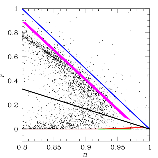
Figure 3: Models generated by Monte Carlo plotted on the $(r,n)$ plane (black dots). The colored lines are the same models as in Fig. 2. For comparison with the models, points are plotted to first order in slow roll.

The final result following the evaluation of a particular path in the $M$-dimensional “slow roll space” is a point in “observable parameter space,” i.e., $(r,n,dn/d\ln k)$, corresponding to the observational prediction for that particular model. This process can be repeated for a large number of models, and used to study the attractor behavior of the inflationary dynamics. In fact, the models cluster strongly in the observable parameter space kinney02 . Figure 3 shows an ensemble of models generated stochastically on the $(r,n)$ plane, along with the predictions of the specific models considered in Sec. III.

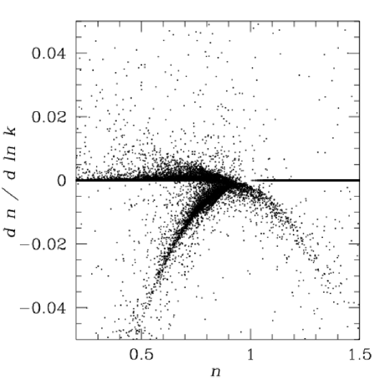
Figure 4: Models generated by Monte Carlo plotted on the $(n,dn/d\ln k)$ plane. Points are plotted to second order in slow roll.

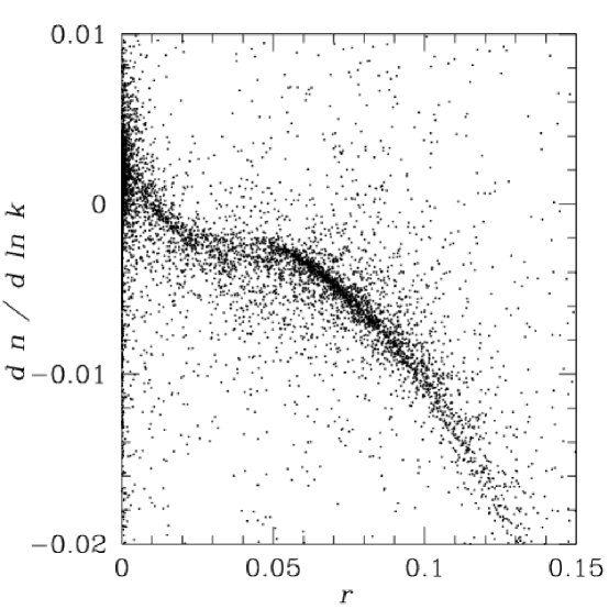
Figure 5: Models generated by Monte Carlo plotted on the $(r,dn/d\ln k)$ plane. Points are plotted to second order in slow roll.

Figure 4 shows an ensemble of models generated stochastically on the $(n,dn/d\ln k)$ plane. As one can see, and contrary to what commonly believed, there are single-field models of inflation which predict a significant running of the spectral index. The same can be appreciated in Fig. 5, where we plot an ensemble of models generated stochastically on the $(r,dn/d\ln k)$ plane.

The reconstruction method works as follows:

1. Specify a “window” of parameter space: e.g., central values for $n-1$, $r$, or $dn/d\ln{k}$ and their associated error bars.

2. Select a random point in slow roll space, $[\epsilon,\eta,{}^{\ell}\lambda_{\rm H}]$, truncated at order $M$ in the slow roll expansion.

3. Evolve forward in time ($dN<0$) until either (a) inflation ends ($\epsilon>1$), or (b) the evolution reaches a late-time fixed point ($\epsilon={}^{\ell}\lambda_{\rm H}=0,\ \sigma={\rm const.}$).

4. If the evolution reaches a late-time fixed point, calculate the observables $r$, $n-1$, and $dn/d\ln k$ at this point.

5. If inflation ends, evaluate the flow equations backward $N$ e-folds from the end of inflation. Calculate the observable parameters at that point.

6. If the observable parameters lie within the specified window of parameter space, compute the potential and add this model to the ensemble of “reconstructed” potentials.

7. Repeat steps 2 through 6 until the desired number of models have been found.

The condition for the end of inflation is that $\epsilon=1$. Integrating the flow equations forward in time will yield two possible outcomes. One possibility is that the condition $\epsilon=1$ may be satisfied for some finite value of $N$, which defines the end of inflation. We identify this point as $N=0$ so that the primordial fluctuations are actually generated when $N\sim 60$. Alternatively, the solution can evolve toward an inflationary attractor with $r=0$ and $n>1$, in which case inflation never stops. In reality, inflation must stop at some point, presumably via some sort of instability, such as the “hybrid” inflation mechanism linde91 ; linde94 ; copeland94 . Here we make the simplifying assumption that the observables for such models are the values at the late-time attractor.

Given a path in the slow roll parameter space, the form of the potential is fixed, up to normalization hodges90 ; copeland93 ; beato00 ; easther02 . The starting point is the Hamilton-Jacobi equation,

$$V(\phi)=\left({3m_{\rm Pl}^{2}}\over 8\pi\right)H^{2}(\phi)\left[1-{1\over 3}\epsilon(\phi)\right].$$ (61)

We have $\epsilon(N)$ trivially from the flow equations. In order to calculate the potential, we need to determine $H(N)$ and $\phi(N)$. With $\epsilon$ known, $H(N)$ can be determined by inverting the definition of $\epsilon$, Eq. (43). Similarly, $\phi(N)$ follows from the first Hamilton-Jacobi equation (6):

$${d\phi\over dN}={m_{\rm PL}\over 2\sqrt{\pi}}\sqrt{\epsilon}.$$ (62)

Using these equations and Eq. (61), the form of the potential can then be fully reconstructed from the numerical solution for $\epsilon(N)$. The only necessary observational input is the normalization of the Hubble parameter $H$, which enters the above equations as an integration constant. Here we use the simple condition that the density fluctuation amplitude (as determined by a first-order slow roll expression) be of order $10^{-5}$,

$${\delta\rho\over\rho}\simeq\frac{1}{2\pi}{H\over m_{\rm Pl}}\frac{1}{\sqrt{\epsilon}}=10^{-5}.$$ (63)

A more sophisticated treatment would perform a full normalization to the COBE CMB data bunn94 ; stompor95 . The value of the field, $\phi$, also contains an arbitrary, additive constant.

V CMB Analysis

Our analysis method is based on the computation of a likelihood distribution over a fixed grid of pre-computed theoretical models. We restrict our analysis to a flat, adiabatic, $\Lambda$-CDM model template computed with CMBFAST (sz ), sampling the parameters as follows: $\Omega_{cdm}h^{2}\equiv\omega_{cdm}=0.01,...0.25$, in steps of $0.01$; $\Omega_{b}h^{2}\equiv\omega_{b}=0.009,...,0.028$, in steps of $0.001$ and $\Omega_{\Lambda}=0.5,...,0.95$, in steps of $0.05$. The value of the Hubble constant is not an independent parameter, since:

$$h=\sqrt{{\omega_{cdm}+\omega_{b}}\over{1-\Omega_{\Lambda}}},$$ (64)

and we use the further prior: $h=0.72\pm 0.15$. We allow for a reionization of the intergalactic medium by varying the Compton optical depth parameter $\tau_{c}$ in the range $\tau_{c}=0.05,...,0.30$ in steps of $0.05$. Our choice of the above parameters is motivated by Big Bang Nucleosynthesis bounds on $\omega_{b}$ (both from D burles and ${}^{4}\textrm{He}+^{7}\textrm{Li}$ cyburt ), from supernovae (super1 ) and galaxy clustering observations (see e.g., thx ), and by the WMAP temperature-polarization cross-correlation data, which indicate an optical depth $\tau=0.17\pm 0.04$ (kogutt ). Our choice for an upper limit of $\tau_{c}<0.30$ is very conservative respect to the maximum values expected in numerical simulations (see e.g., ciardi ) even in the case of non-standard reionization processes. From the grid above, we only consider models with an age of the universe in excess of 11 Gyr. Variations in the inflationary parameters $n$, $r$ and $dn/d\ln{k}$ are not computationally relevant, and for the range of values we considered they can be assumed as free parameters. The tensor spectral index $n_{t}$ is determined by the consistency relation.

For the WMAP data we use the recent temperature and cross polarization results from Ref. wmap1 and compute the likelihood ${\cal L}^{WMAP}$ for each theoretical model as explained in Ref. Verde:2003ey , using the publicly available code on the LAMBDA web site (http://lambda.gsfc.nasa.gov/).

We further include the results from seven other experiments: BOOMERanG-98 ruhl , MAXIMA-1 lee , DASI halverson , CBI cbi , ACBAR acbar , VSAE grainge , and Archeops benoit . The expected theoretical Gaussian signal inside the bin $C_{B}^{th}$ is computed by using the publicly available window functions and lognormal prefactors as in Ref. BJK . The likelihood ${\cal L}^{pre-WMAP}$ from this dataset and for a given theoretical model is defined by

$$-2\ln{\cal L}^{pre-WMAP}=(C_{B}^{th}-C_{B}^{ex})M_{BB^{\prime}}(C_{B^{\prime}}^{th}-C_{B^{\prime}}^{ex}),$$ (65)

where $M_{BB^{\prime}}$ is the Gaussian curvature of the likelihood matrix at the peak and $C_{B}^{ex}$ is the experimental signal in the bin. We consider $7\%$, $10\%$, $4\%$, $5\%$, $5\%$, $5\%$ and $5\%$ Gaussian distributed calibration errors for the Archeops, BOOMERanG-98, DASI, MAXIMA-1, VSAE, ACBAR, and CBI, experiments respectively and include the beam uncertainties using the analytical marginalization method presented in bridle . We use as combined likelihood just the normalized product of the two likelihood distributions: ${\cal L}\sim{\cal L}^{WMAP}\times{\cal L}^{pre-WMAP}$.

In order to constrain a set of parameters $\vec{x}$ we marginalize over the values of the remaining “nuisance” parameters $\vec{y}$. This yields the marginalized likelihood distribution

$$\mathcal{L}(\vec{x})\equiv P(\vec{x}|{\cal C}_{B})=\int{\cal L}(\vec{x},\vec{y})d\vec{y}.$$ (66)

In the next section we will present constraints in several two-dimensional planes. To construct plots in two dimensions, we project (not marginalize) over the third, “nuisance” parameter. For example, likelihoods in the $(r,n)$ plane are calculated for given choice of $r$ and $n$ by using the value of $dn/d\ln{k}$ which maximizes the likelihood function. The error contours are then plotted relative to likelihood falloffs of $0.17$, $0.018$ and $0.0035$ as appropriate for $1\sigma$, $2\sigma$, and $3\sigma$ contours of a three-dimensional Gaussian. In effect we are taking the shadow of the three-dimensional error contours rather than a slice, which makes clear the relationship between the error contours and the points generated by Monte Carlo. All likelihoods used to constrain models are calculated relative the the full three-dimensional likelihood function.

VI Results

We will plot the likelihood contours obtained from our analysis on three different planes: $dn/d\ln{k}$ vs. $n$, $r$ vs. $n$ and $r$ vs. $dn/d\ln{k}$. Presenting our results on these planes is useful for understanding the effects of theoretical assumptions and/or external priors.

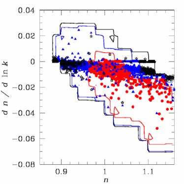
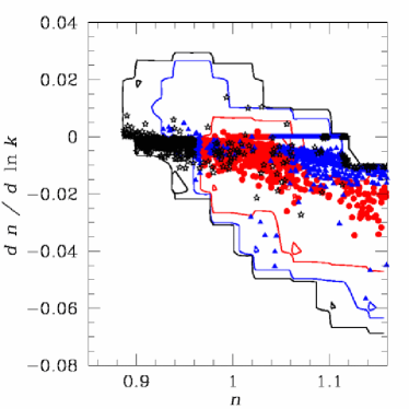
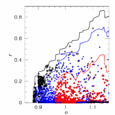
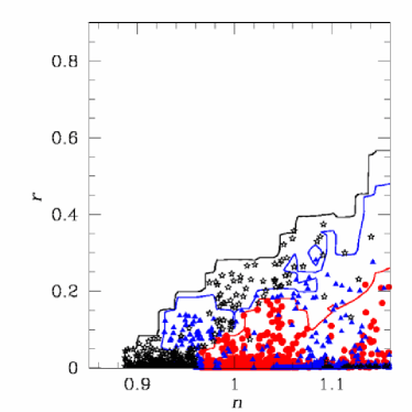
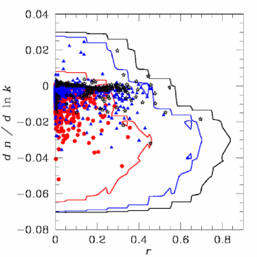
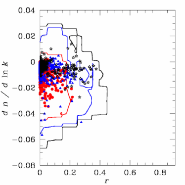
Figure 6: Likelihood contours for WMAP alone (left column) and WMAP plus seven other experiments (right column), plotted in the ($n,dn/d\ln{k}$) plane (top), the ($n,r$) plane (center), and the ($r,dn/d\ln{k}$) plane (bottom). The points represent the results of the Monte Carlo sampling of inflationary models consistent with $1\sigma$ (red, dots), $2\sigma$ (blue, triangles), and $3\sigma$ (black, stars) contours. All points in this and subsequent figures are plotted to second order in slow roll.

We do this in Fig. 6 for two cases: the WMAP dataset alone (left column), and WMAP plus the additional CMB experiments BOOMERanG-98, MAXIMA-1, DASI, CBI, ACBAR, VSAE, and Archeops (right column). By analyzing these different datasets we can check the consistency of the previous experiments with WMAP. The dots superimposed on the likelihood contours show the models sampled by the Monte Carlo reconstruction.

In the top row of Fig. 6, we show the 68%, 95%, and 99% likelihood contours on the $n$ vs. $dn/d\ln{k}$ plane (refer to the end of Sec. V for a discussion of the method used to plot the contours.) The pivot scale $k_{0}$ is $k_{0}=0.002h$ Mpc^-1. As we can see, both datasets are consistent with a scale invariant $n=1$ power law spectrum with no further scale dependence ($dn/d\ln{k}=0$). A degeneracy is also evident: an increase in the spectral index $n$ is equivalent to a negative scale dependence ($dn/d\ln{k}<0$). We emphasize, however, that this beahavior depends strictly on the position of the pivot scale $k_{0}$: choosing $k_{0}=0.05h$ Mpc^-1 would change the direction of the degeneracy. Models with $n\sim 1.1$ need a negative running at about the $3\sigma$ level. It is interesting also to note that models with lower spectral index, $n\sim 0.9$, are in better agreement with the data with a zero or positive running. For $n<1$, the running is bounded by $0.005\gtrsim dn/d\ln{k}\gtrsim-0.025$ at $1\sigma$.

In the center row of Fig. 6 we plot the 68%, 95%, and 99% likelihood contours on the $r$ vs. $n$ plane. As we can see, the present data only weakly constrain the presence of tensor modes, although a gravity wave component is not preferred. Models with $n<0.9$ must have a negligible tensor component, while models with $n>1$ can have $r$ larger than $0.4$ ($2\sigma$ C.L.). However, as we can see from the bottom row of Fig. 6, there is no correlation between the tensor component and the running of the scalar index.

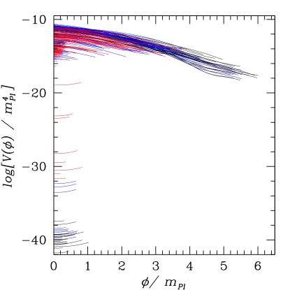
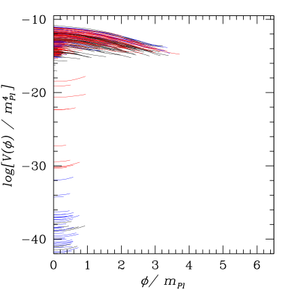
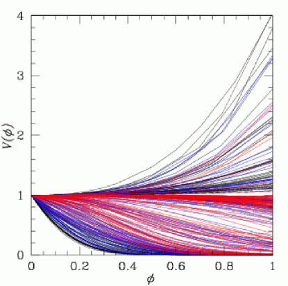
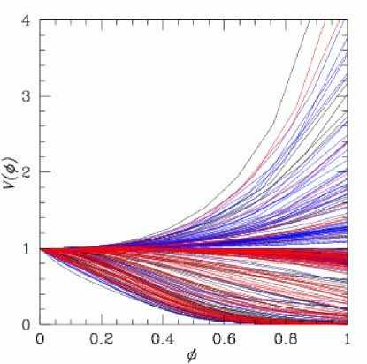
Figure 7: Three hundred reconstructed potentials chosen from the sampling shown in Fig. 6 for the WMAP dataset (left column) and the WMAP data set plus seven other experiments (right column). The potentials are color-coded according to their likelihoods: $1\sigma$ (red) $2\sigma$ (blue), and $3\sigma$ (black). The top figure shows the potentials with height and width plotted in units of $m_{\rm Pl}$, and the bottom figure shows the same potentials rescaled to all have the same height and width.

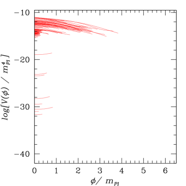
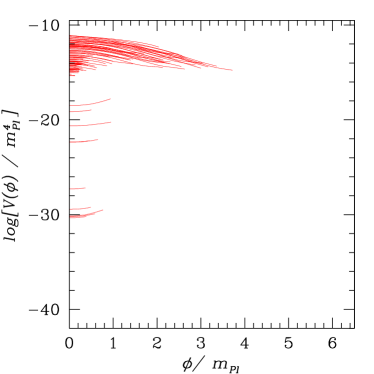
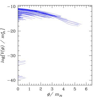
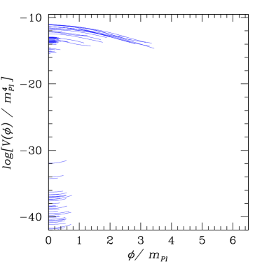
Figure 8: Reconstructed potentials from Fig. 7 plotted separately by likelihood: $1\sigma$ (red, top), $2\sigma$ (blue, center), and $3\sigma$ (black, bottom). The WMAP results are in the left column, and WMAP plus seven other experiments are in the right column.

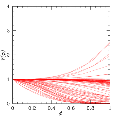
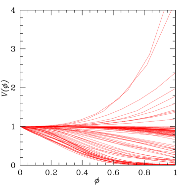
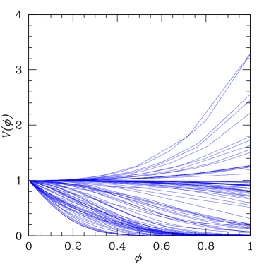
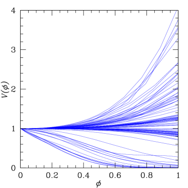
Figure 9: Same as Fig. 8, but with the potentials rescaled to all have the same height and width.

Figures 7, 8, and 9 show a subset of 300 reconstructed potentials selected from the sampled set. Note in particular the wide range of inflationary energy scales compatible with the observational constraint. This is to be expected, since there was no detection of tensor modes in the WMAP data, which would be seen here as a detection of a nonzero tensor/scalar ratio $r$. In addition, the shape of the inflationary potential is also not well constrained by WMAP.

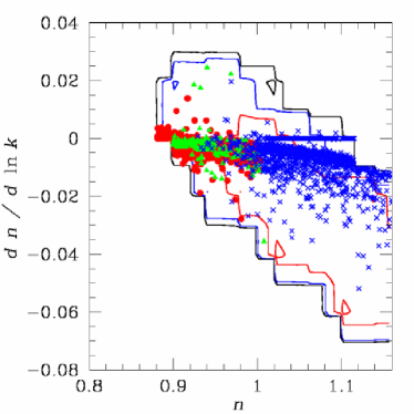
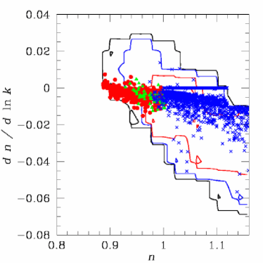
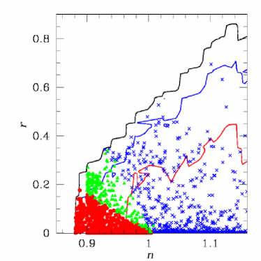
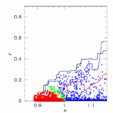
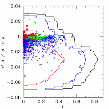
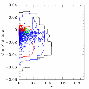
Figure 10: Likelihood contours plotted in the ($n,dn/d\ln{k}$) plane (top), the ($n,r$) plane (center), and the ($r,dn/d\ln{k}$) plane (bottom). The points represent the results of the Monte Carlo sampling, color coded by model type: small-field (red, dots), large-field (green, triangles), and hybrid (blue, crosses). The left column is WMAP only while the right column is WMAP plus seven other experiments

Figure 10 shows the models sampled by the Monte Carlo categorized by their “zoology”, i.e., whether they fit into the category of small-field, large-field, or hybrid. We see that all three types of potential are compatible with the data, although hybrid class models are preferred by the best-fit region.

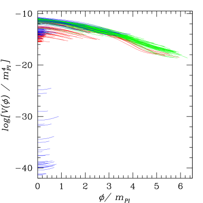
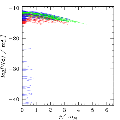
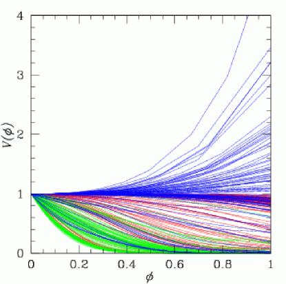
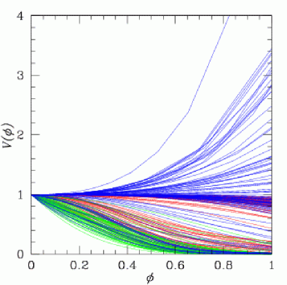
Figure 11: Three hundred reconstructed potentials chosen from the sampling shown in Fig. 6 for WMAP (left column) and WMAP plus seven other experiments (right column). The potentials are color-coded according to model type: small-field (red), large-field (green), and hybrid (blue). The top figure shows the potentials with height and width plotted in units of $m_{\rm Pl}$, and the bottom figure shows the same potentials rescaled to all have the same height and width.

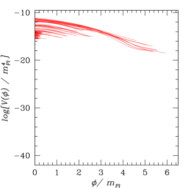
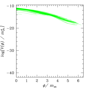
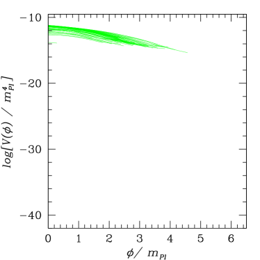
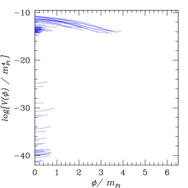
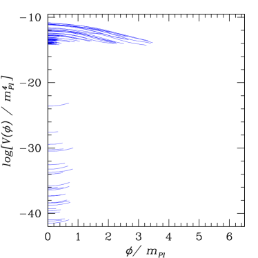
Figure 12: Reconstructed potentials from Fig. 11 plotted separately by model type: small-field (red, top), large-field (green, center), and hybrid (blue, bottom). The WMAP results are shown in the left column while WMAP plus seven other experiments are shown onthe right column.

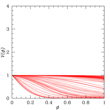
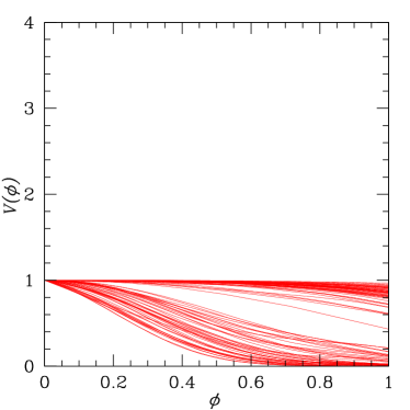
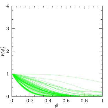
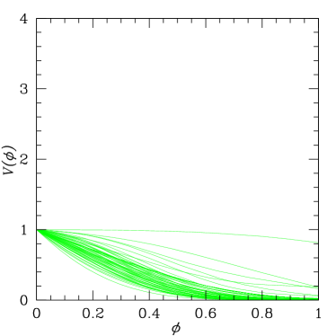
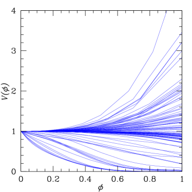
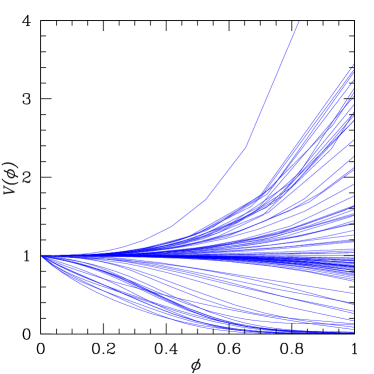
Figure 13: Same as Fig. 12, but with the potentials rescaled to all have the same height and width.

Figures 11, 12, and 13 show the reconstructed potentials divided by type. Perhaps the only conclusion to be drawn here is that the WMAP data places no significant constraint on the shape of the inflationary potential; many “reasonable” potentials are consistent with the data. However, significant portions of the observable parameter space are ruled out by WMAP, and future observations can be expected to significantly tighten these constraints dodelson97 ; kinney98a .

For the particular example of $V\propto\phi^{4}$, using Eq. 58 we find that this choice of potential ruled out to $3\sigma$ only for $N<40$ for the WMAP data set. This constraint is even weaker than that claimed by Barger et al. barger , most likely because we allow for a running of the spectral index in our constraint.

When augmenting the WMAP data set with the data from seven other CMB experiments, the most noticeable improvement in the constraints is a better upper limit to the tensor/scalar ratio $r$, which results in a slightly improved upper limit on the height of the potential. Also, the width of the reconstructed potentials in Planck units is somewhat less than in the case of the WMAP-only constraint, showing that the additional data more strongly limit the form of the inflationary potential.

The combined data rules out a potential with $V\propto\phi^{4}$ for $N<66$ to $3\sigma$, effectively killing such models as observationally viable candidates for the inflaton potential.

VII Conclusions

In this paper, we presented an analysis of the WMAP data set with an emphasis on parameters relevant for distinguishing among the various possible models for inflation. In contrast to previous analyses, we confined ourselves to CMB data only and performed a likelihood analysis over a grid of models including the full error covariance data from the WMAP satellite alone, and in conjunction with measurements from BOOMERanG-98, MAXIMA-1, DASI, CBI, ACBAR, VSAE, and Archeops.

We found that the WMAP data alone are consistent with a scale-invariant power spectrum, $n=1$, with no running of the spectral index, $dn/d\ln{k}=0$. However, a great number of models indicates a compatibility of the data with a blue spectral index and a substantial negative running. This is consistent with the result published by the WMAP team including data from large-scale structure measurements and the Lyman-$\alpha$ forest. The WMAP result is also consistent with previous CMB experiments. The inclusion of previous datasets in the analysis has the effect of reducing the error bars and give a better determination of the inflationary parameters. Still, no clear evidence for the running is present in the combined analysis. This result differs from the result obtained in Peiris et al. in the case of combined (WMAP+CBI+ACBAR) analysis, where a mild (about $1.5\sigma$) evidence for running was reported. The different and more conservative method of analysis adopted here, and the larger CMB dataset used in our paper can explain this difference.

In addition, we applied the Monte Carlo reconstruction technique to generate an ensemble of inflationary potentials consistent with observation. Of the three basic classes of inflation model, small-field, large-field, and hybrid, none are conclusively ruled out, although hybrid models are favored by the best fit region. The reconstruction process indicates that a wide variety of smooth potentials for the inflaton are consistent with the data, indicating that the WMAP result is too crude to significantly constrain either the height or the shape of the inflaton potential. In particular, the lack of evidence for tensor fluctuations makes it impossible to constrain the energy scale at which inflation takes place. Nonetheless, WMAP rules out a large portion of the available parameter space for inflation, itself a significant improvement over previous measurements. For the particular case of a potential of the form $V\left(\phi\right)=\lambda\phi^{4}$, WMAP rules out all such potentials for $N<40$ at the $3\sigma$ level, which means that $\phi^{4}$ potentials are not conclusively ruled out by WMAP alone. The combined data set, however, rules out $\phi^{4}$ models for $N<66$, which kills such potentials as viable candidates for inflation.

After this paper first appeared, Leach and Liddle also released a reanalysis of the WMAP data leach03 , which is in general agreement with our results here.

WMAP only                            WMAP plus seven other experiments

        

        

        

WMAP only                            WMAP plus seven other experiments

        

        

WMAP only                            WMAP plus seven other experiments

        

        

        

WMAP only                            WMAP plus seven other experiments

        

        

        

WMAP only                            WMAP plus seven other experiments

        

        

        

WMAP only                            WMAP plus seven other experiments

        

        

WMAP only                            WMAP plus seven other experiments

        

        

        

WMAP only                            WMAP plus seven other experiments

References

- (1) A. Guth, Phys. Rev. D 23, 347 (1981)
- (2) D. H. Lyth and A. Riotto, Phys. Rept. 314 1 (1999); A. Riotto, hep-ph/0210162; W. H. Kinney, astro-ph/0301448.
- (3) V. F. Mukhanov and G. V. Chibisov, JETP Lett. 33, 532 (1981).
- (4) S. W. Hawking, Phys. Lett. 115B, 295 (1982).
- (5) A. Starobinsky, Phys. Lett. 117B, 175 (1982).
- (6) A. Guth and S. Y. Pi, Phys. Rev. Lett. 49, 1110 (1982).
- (7) J. M. Bardeen, P. J. Steinhardt, and M. S. Turner, Phys. Rev. D 28, 679 (1983).
- (8) G. F. Smoot et al. Astrophys. J. 396, L1 (1992).
- (9) C. L. Bennett et al. Astrophys. J. 464, L1 (1996).
- (10) K. M. Gorski et al. Astrophys. J. 464, L11 (1996).
- (11) See, for example, N. Bahcall, J. P. Ostriker, S. Perlmutter and P. J. Steinhardt, Science 284, 1481 (1999).
- (12) E. Torbet et al., Astrophys. J. 521 (1999) L79, astro-ph/9905100; A. D. Miller et al., Astrophys. J. 524 (1999) L1, astro-ph/9906421.
- (13) P. D. Mauskopf et al. [Boomerang Collaboration], Astrophys. J. 536 (2000) L59, astro-ph/9911444; A. Melchiorri et al. [Boomerang Collaboration], Astrophys. J. 536 (2000) L63 astro-ph/9911445.
- (14) C. B. Netterfield et al. [Boomerang Collaboration], astro-ph/0104460.
- (15) N. W. Halverson et al., astro-ph/0104489.
- (16) P. F. Scott et al., astro-ph/0205380.
- (17) A. Benoit, astro-ph/0210305.
- (18) T. J. Pearson et al., astro-ph/0205388.
- (19) P. de Bernardis et al., [Boomerang Collaboration], astro-ph/0105296.
- (20) C. Pryke, N. W. Halverson, E. M. Leitch, J. Kovac, J. E. Carlstrom, W. L. Holzapfel and M. Dragovan, astro-ph/0104490.
- (21) R. Stompor et al., Astrophys. J. 561 (2001) L7, astro-ph/0105062.
- (22) X. Wang, M. Tegmark, M. Zaldarriaga, astro-ph/0105091.
- (23) J. L. Sievers et al., astro-ph/0205387.
- (24) J. A. Rubino-Martin et al., astro-ph/0205367.
- (25) A. Lewis and S. Bridle, astro-ph/0205436.
- (26) A. Melchiorri and J. Silk, astro-ph/0203200; S. H. Hansen, G. Mangano, A. Melchiorri, G. Miele and O. Pisanti, Phys. Rev. D 65, 023511 (2002), astro-ph/0105385; A. Melchiorri, L. Mersini, C. J. Odman and M. Trodden, astro-ph/0211522.
- (27) C. J. Odman, A. Melchiorri, M. P. Hobson and A. N. Lasenby, astro-ph/0207286.
- (28) S. Dodelson, W. H. Kinney, and E. W. Kolb, Phys. Rev. D 56, 3207 (1997), astro-ph/9702166.
- (29) W. H. Kinney, Phys. Rev. D 58, 123506 (1998).
- (30) W. H. Kinney, A. Melchiorri, A. Riotto, Phys. Rev. D 63, 023505 (2001), astro-ph/0007375; S. Hannestad, S. H. Hansen, and F. L. Villante, Astropart. Phys. 17 375 (2002); S. Hannestad, S. H. Hansen and F. L. Villante, Astropart. Phys. 16, 137 (2001); D. J. Schwarz, C. A. Terrero-Escalante, and A. A. Garcia, Phys. Lett. B 517, 243 (2001); X. Wang, M. Tegmark, B. Jain and M. Zaldarriaga, astro-ph/0212417.
- (31) C. L. Bennett et al., astro-ph/0302207.
- (32) Kogut et al, astro-ph/0302213.
- (33) H. V. Peiris et al., astro-ph/0302225.
- (34) V. Acquaviva, N. Bartolo, S. Matarrese and A. Riotto, astro-ph/0209156; J. Maldacena, astro-ph/0210603.
- (35) E. Komatsu et al., astro-ph/0302223.
- (36) W. H. Kinney, Phys. Rev. D 66, 083508 (2002), astro-ph/0206032.
- (37) R. Easther and W. H. Kinney, Phys. Rev. D 67, 043511 (2003), astro-ph/0210345.
- (38) V. Barger, H. S. Lee and D. Marfatia, hep-ph/0302150.
- (39) C.L. Kuo et al., astro-ph/0212289.
- (40) W.J. Percival et al., astro-ph/0105252.
- (41) R.A. Croft et al., Astrophys. J. 581, 20 (2002); N.Y. Gnedin and A.J. Hamilton, astro-ph/0111194.
- (42) W.L. Freedman et al., Astrophys. J. 553, 47 (2001).
- (43) J. E. Ruhl et al. [Boomerang Collaboration], astro-ph/0212229.
- (44) A. T. Lee et al., Astrophys. J. 561, L1 (2001), astro-ph/0104459.
- (45) K. Grainge et al., astro-ph/0212495.
- (46) A. D. Linde, Phys. Lett. 129B, 177 (1983).
- (47) K. Freese, J. Frieman, and A. Olinto, Phys. Rev. Lett 65, 3233 (1990).
- (48) A. D. Linde, Phys. Lett. 259B, 38 (1991).
- (49) A. D. Linde, Phys. Rev. D 49, 748 (1994).
- (50) E. J. Copeland, A. R. Liddle, D. H. Lyth, E. D. Stewart, and D. Wands, Phys. Rev. D 49, 6410 (1994).
- (51) A. A. Starobinsky, Phys. Lett. 91B, 99 (1980).
- (52) L. P. Grishchuk and Yu. V. Sidorav, in Fourth Seminar on Quantum Gravity, eds M. A. Markov, V. A. Berezin and V. P. Frolov (World Scientific, Singapore, 1988).
- (53) A. G. Muslimov, Class. Quant. Grav. 7, 231 (1990).
- (54) D. S. Salopek and J. R. Bond, Phys. Rev. D 42, 3936 (1990).
- (55) J. E. Lidsey et al., Rev. Mod. Phys. 69, 373 (1997), astro-ph/9508078.
- (56) J. E. Lidsey, A. R. Liddle, E. W. Kolb, E. J. Copeland, T. Barriero, and M. Abney, Rev. Mod. Phys. 69, 373 (1997).
- (57) S. Dodelson and L. Hui, astro-ph/0305113.
- (58) A. D. Linde, Phys. Lett. B108 389, 1982.
- (59) A. Albrecht and P. J. Steinhardt, Phys. Rev. Lett 48, 1220 (1982).
- (60) W. H. Kinney, Phys. Rev. D 56 2002 (1997), hep-ph/9702427.
- (61) V. F. Mukhanov, JETP Lett. 41, 493 (1985).
- (62) V. F. Mukhanov, Sov. Phys. JETP 67, 1297 (1988).
- (63) V. F. Muknanov, H. A. Feldman, and R. H. Brandenberger, Phys. Rep. 215, 203 (1992).
- (64) E. D. Stewart and D. H. Lyth, Phys. Lett. 302B, 171 (1993).
- (65) E. D. Stewart, Phys. Lett. B391, 34 (1997), hep-ph/9606241.
- (66) A. D. Linde and A. Riotto, Phys. Rev. D 56, 1841 (1997), hep-ph/9703209.
- (67) E. D. Stewart, Phys. Rev. D 56, 2019 (1997), hep-ph/9703232.
- (68) E. J. Copeland, I. J. Grivell, and A. R. Liddle, astro-ph/9712028.
- (69) W. H. Kinney and A. Riotto, Astropart. Phys. 10, 387 (1999), hep-ph/9704388.
- (70) L. Covi, D. H. Lyth and L. Roszkowski, Phys. Rev. D 60, 023509 (1999), hep-ph/9809310.
- (71) W. H. Kinney and A. Riotto, Phys. Lett.435B, 272 (1998), hep-ph/9802443.
- (72) L. Covi and D. H. Lyth, Phys. Rev. D 59 (1999) 063515, hep-ph/9809562.
- (73) D. H. Lyth and L. Covi, astro-ph/0002397.
- (74) A. A. Starobinski, Grav. Cosmol. 4, 88 (1998), astro-ph/9811360. D. J. Chung, E. W. Kolb, A. Riotto and I. I. Tkachev, hep-ph/9910437.
- (75) A. A. Starobinsky, JETP Lett. 30, 682 (1979).
- (76) V. Rubakov, M. Sazhin, and A. Veryaskin, Phys. Lett. 115B, 189 (1982).
- (77) R. Fabbri and M. Pollock, Phys. Lett. 125B, 445 (1983).
- (78) L.F. Abbott and M.B. Wise, Nucl. Phys. B244, 541 (1984).
- (79) A .A. Starobinsky, Sov. Astron.Lett. 11, 133 (1985).
- (80) E. F. Bunn and M. White, Astrophys. J. 480, 6 (1997).
- (81) D. H. Lyth, hep-ph/9609431.
- (82) D. Polarski and A. A. Starobinsky, Phys. Lett. 356B, 196 (1995).
- (83) J. García-Bellido and D. Wands, Phys. Rev. D 52, 6739 (1995).
- (84) M. Sasaki and E. D. Stewart, Prog. Theor. Phys. 95, 71 (1996).
- (85) J. García-Bellido, Phys. Lett. 418B, 252 (1998).
- (86) J. D. Barrow and A. R. Liddle, Phys. Rev. D 47, R5219 (1993).
- (87) A. R. Liddle, P. Parsons, and J. D. Barrow, Phys. Rev. D 50, 7222 (1994), astro-ph/9408015.
- (88) M. B. Hoffman and M. S. Turner, Phys. Rev. D 64, 023506 (2001), astro-ph/0006321.
- (89) D. J. Schwarz, C. A. Terrero-Escalante, and A. .A. Garcia, Phys. Lett. B517, 243 (2001), astro-ph/0106020.
- (90) A. R. Liddle. and M. S. Turner, Phys. Rev. D 50, 758 (1994).
- (91) H. M. Hodges and G. R. Blumenthal, Phys. Rev. D 42, 3329 (1990).
- (92) E. J. Copeland et al. Phys. Rev. Lett. 71, 219 (1993).
- (93) E. Ayon-Beato, A. Garcia, R. Mansilla, and C. A. Terrero-Escalante, Phys. Rev. D 62, 103513 (2000).
- (94) E. F. Bunn, D. Scott, and M. White, Astrophys. J. Lett. 441, L9 (1995), astro-ph/9409003.
- (95) R. Stompor, K. M. Gorski and A. J. Banday, Mon. Not. R. Astron. Soc. 277, 1225 (1995), astro-ph/9502035.
- (96) M. Zaldarriaga and U. Seljak, Astrophys. J. 469, 437 (1996), astro-ph/9603033.
- (97) S. Burles, K. M. Nollett and M. S. Turner, Astrophys. J. 552, L1 (2001), astro-ph/0010171.
- (98) R. H. Cyburt, B. D. Fields and K. A. Olive, Compilation and Big Bang Nucleosynthesis,” New Astron. 6 (1996) 215, astro-ph/0102179.
- (99) P.M. Garnavich et al, Ap.J. Letters 493, L53-57 (1998); S. Perlmutter et al, Ap. J. 483, 565 (1997); S. Perlmutter et al (The Supernova Cosmology Project), Nature 391 51 (1998); A.G. Riess et al, Ap. J. 116, 1009 (1998);
- (100) M. Tegmark, A. J. S. Hamilton, Y. Xu, astro-ph/0111575.
- (101) B. Ciardi, A. Ferrara and S. D. M. White, astro-ph/0302451.
- (102) L. Verde et al., astro-ph/0302218.
- (103) Bond, J.R., Jaffe, A.H., & Knox, L.E. 2000, Astrophys. J. , 533, 19
- (104) S. L. Bridle, R. Crittenden, A. Melchiorri, M. P. Hobson, R. Kneissl and A. N. Lasenby, astro-ph/0112114.
- (105) S. M. Leach and A. R. Liddle, astro-ph/0306305.