hep-ph/0305129 DFPD-03/TH/16

SACLAY-T03/059

UG-FT-150/03

CAFPE-20-03

Fermion Generations, Masses and Mixing Angles
from Extra Dimensions

Carla Biggio     Ferruccio Feruglio 

Dipartimento di Fisica ‘G. Galilei’, Università di Padova

INFN, Sezione di Padova, Via Marzolo 8, I-35131 Padua, Italy

Isabella Masina ^,

Service de Physique Théorique CEA/Saclay

Orme des Merisiers F-91191 Gif-sur-Yvette Cedex, France

Manuel Pérez-Victoria 

Dipartimento di Fisica ‘G. Galilei’, Università di Padova

INFN, Sezione di Padova, Via Marzolo 8, I-35131 Padua, Italy

Departamento de Física Teórica y del Cosmos

Centro Andaluz de Física de Partículas Elementales (CAFPE)

Universidad de Granada, E-18071 Granada, Spain

We discuss a toy model in six dimensions that predicts two fermion generations, natural mass hierarchy and intergenerational mixing. Matter is described by vector-like six dimensional fermions, one per each irreducible standard model representation. Two fermion generations arise from the compactification mechanism, through orbifold projection. They are localized in different regions of the compact space by a six dimensional mass term. Flavour symmetry is broken via Yukawa couplings, with a Higgs vacuum expectation value not constant in the extra space. A hierarchical spectrum is obtained from order one dimensionless parameters of the six dimensional theory. The Cabibbo angle arises from the soft breaking of six dimensional parity symmetry. We also briefly discuss how the present model could be extended to cover the realistic case.

In the last years our knowledge in flavour in physics has undergone a spectacular development. On the experimental side, with the data from the existing B factories, BABAR and Belle, we entered an era of precision tests in the quark sector. For instance the $|V_{cb}|$ element of the quark mixing matrix is now known with a precision of few percents [1]. Moreover many independent measurements are now over-constraining the quark parameters of the standard model (SM), and the success of the theory in fitting all the data is really impressive. Also the picture in the lepton sector has been greatly clarified and, even if we have not yet obtained precise determination of mass and mixing parameters, nevertheless a clear pattern has been identified from the solutions to the solar and atmospheric neutrino problems [2].

On the theoretical side, we should honestly admit that flavour still represents one of the great mysteries in particle physics. We do not know the scale at which the flavour dynamics sets in. Perhaps at this scale a conventional, four dimensional, picture still holds thus allowing us to analyze the flavour problem in the context of a local quantum field theory in four space-time dimensions. Here the most powerful tool that we have to decipher the observed hierarchy among the different masses and mixing angles is that of spontaneously broken flavour symmetries [3]. In the idealized limit of exact symmetry, only the heaviest fermions are massive: the top quark and, maybe, the whole third family. The lightest fermions and the small mixing angles originate from breaking effects. This beautiful idea has been widely explored in many possible versions, with discrete or continuous symmetries, global or local ones. A realistic description of fermion masses in this framework typically requires either a large number of parameters or a high degree of complexity and we are probably unable to select the best model among the many existing ones. Moreover, in four dimensions we have little hopes to understand why there are exactly three generations.

It might be the case that at the energy scale characterizing flavour physics a four-dimensional description breaks down. For instance this happens in superstring theories where the space-time is ten or eleven dimensional. In the ten dimensional heterotic string six dimensions can be compactified on a Calabi-Yau manifold [4] or on orbifolds [5] and the flavour properties are strictly related to the features of the compact space. In Calabi-Yau compactifications the number of chiral generations is proportional to the Euler characteristics of the manifold. In orbifold compactifications, matter in the twisted sector is localized around the orbifold fixed points and the Yukawa couplings, arising from world-sheet instantons, have a natural geometrical interpretation [6]. Recently string realizations where the light matter fields of the standard model arises from intersecting branes have been proposed. Also in this context the flavour dynamics is controlled by topological properties of the geometrical construction [7], having no counterpart in four dimensional field theories.

Perhaps in the future the flavour mystery will be unraveled by string theory, but in the meantime it would be interesting to explore, in a pure field theoretical construction, the possibility of extra space-like dimensions. We can then take advantage of the greater freedom that a bottom-up field-theory approach possesses compared to string theory. Moreover in the last years a lot of progress has been done in understanding field theories with extra spatial dimensions. These theories are ultraviolet divergent and should be cut-off at some energy scale $\Lambda$, but they can still be useful as effective descriptions at low energies, including the compactification scale. Semi-realistic models have been proposed within orbifold compactification, allowing for light chiral fermions [8, 9]. The compactification mechanism and the orbifold projection have also been exploited to break supersymmetry [10, 11] and/or gauge symmetry [12, 13] with distinctive and attractive features [14].

It has soon been realized that also in a field theoretical description the existence of extra dimensions could have important consequences for the flavour problem. For instance in orbifold compactifications light four dimensional fermions may be either localized at the orbifold fixed points or they may arise as zero modes of higher-dimensional spinors, with a wave function suppressed by the square root of the volume of the compact space. This led to several interesting proposals. It has been suggested that the smallness of neutrino masses could be reproduced if the left-handed active neutrinos sit at a fixed point and the right-handed sterile partners live in the bulk of a large fifth dimension [15]. In five dimensional grand unified theories the heaviness of the third generation can be explained by localizing the corresponding fields on a fixed point, whereas the relative lightness of the first two generations as well as the breaking of the unwanted mass relations can be obtained by using bulk fields [16].

Even more interesting is the case when a higher dimensional spinor interacts with a non-trivial background of solitonic type. It has been known for a long time that this provides a mechanism to obtain massless four dimensional chiral fermions [17, 18]. Moreover, since the wave functions for the zero modes of the Dirac operator are localized around the core of the topological defect, such a mechanism can play a relevant role in explaining the observed hierarchy in the fermion spectrum [19]. Mass terms arise dynamically from the overlap among fermion and Higgs wave functions. Typically, there is an exponential mapping between the parameters of the higher dimensional theory and the four dimensional masses and mixing angles, so that even with parameters of order one large hierarchies are created [20]. In orbifold compactifications, solitons are simulated by scalar fields with a non-trivial parity assignment that forbids constant non-vanishing vacuum expectation values (VEVs). Under certain conditions, the energy is minimized by field configurations with a non-trivial dependence upon the compact coordinates [21]. Also in this case the zero modes of the Dirac operator in such a background can be chiral and localized in specific regions of the compact space.

In models of this sort, several zero modes can originate from a single higher dimensional spinor [17, 18]. For instance, in the model studied in ref. [22] there is a vortex solution that arises in the presence of two infinite extra dimensions. It is possible to choose the vortex background in such a way that the number of chiral zero modes of the four dimensional Dirac operator is three. Each single six dimensional spinor gives rise to three massless four dimensional modes with the same quantum numbers, thus providing an elegant mechanism for understanding the fermion replica. Recently this model has been extended to the case of compact extra dimensions [23].

In the present work we propose a model where the different fermion generations originate from orbifold compactification, with a natural hierarchy among the fermion masses and with a non-trivial mixing in flavour space. We consider the case of two extra dimensions compactified on the orbifold $T^{2}/Z_{2}$, which allows for a straightforward inclusion of localized gauge fields. Matter is described by vector-like six dimensional fermions with the gauge quantum numbers of one standard model generation. As a result, the model has neither bulk nor localized gauge anomalies. Here we focus on a toy model with two generations, to discuss in a simple setting the features of our proposal and postpone the search for a fully realistic model to a future investigation. The two generations arise as zero modes of the Dirac operator by eliminating the unwanted chiralities of vector-like six dimensional spinors through an orbifold projection. By consistency, the fermion mass is required to be $Z_{2}$-odd and, as a consequence, the two independent zero modes are localized at the opposite sides of the sixth dimension. The two fermion generations are distinguished by localizing the Higgs doublet around $x_{6}=0$. This gives automatically rise to the desired mass hierarchy. A non-trivial flavour mixing also comes out naturally and does not need any additional structure beyond the minimal one. Such a mixing is related to a soft breaking of the six dimensional parity symmetry. In particular, in the quark sector of our toy model, the empirical relation $\theta_{C}\approx\sqrt{m_{d}/m_{s}}$ can be easily accommodated. The essence of our proposal is to address within a unique higher dimensional framework both the problem of fermion replica and that of flavour symmetry breaking. We believe that the model described in the next sections represents a concrete step towards the realization of such a program.

We want to identify the different fermion generations with the appropriate components of a higher dimensional fermion. A five dimensional (5D) fermion contains two 4D components with opposite chirality. After projecting out the wrong chirality we are thus left with a single generation. In 6D fermions can be chiral and a 6D chiral fermion has the same content of a 5D fermion. The simplest conceivable case where two replica with the same 4D chirality are present is that of a 6D vector-like fermion and we will adopt this choice to build a toy model with two fermion generations. To this purpose we consider two extra spatial dimensions compactified on the orbifold $T^{2}/Z_{2}$, where $T^{2}$ is the torus defined by $x_{i}\to x_{i}+2\pi R_{i}$ $(i=5,6)$ and $Z_{2}$ is the parity symmetry $(x_{5},x_{6})\to(-x_{5},-x_{6})$. As fundamental region of the orbifold we can take, for instance, the rectangle $(|x_{5}|\leq\pi R_{5})$, $(0\leq x_{6}\leq\pi R_{6})$ (see fig. 1).

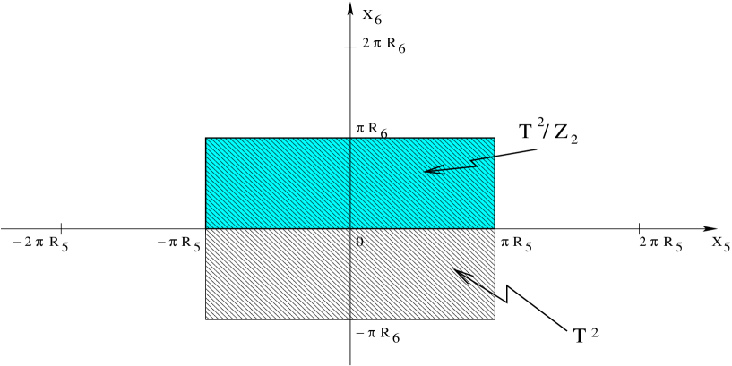
Figure 1: Fundamental region of the orbifold $T^{2}/Z_{2}$.

There are four inequivalent fixed points under $Z_{2}$. In the chosen fundamental region they can be identified with $(x_{5},x_{6})=(0,0)$, $(\pi R_{5},0)$, $(0,\pi R_{6})$, $(\pi R_{5},\pi R_{6})$. Our theory is invariant under the gauge group SU(3)$\otimes$SU(2)$\otimes$U(1). To justify the use of 6D vector-like fermions as building blocks of our model, we also ask invariance under 6D parity to start with. As a consequence, the Lagrangian has 6D vector-like fermions $\Psi^{(\alpha)}$ $(\alpha=1,...5)$, one for each irreducible representation of the SM, as summarized in table 1. With this set of fermion fields, our model is automatically free from 6D gauge anomalies. As we will see later on, requiring exact 6D parity symmetry is too strong an assumption to obtain a ‘realistic’ fermion spectrum. Although eventually we will relax this assumption, for the time being we carry on our construction by enforcing 6D parity invariance.

Table 1: Vector-like 6D fermions and their gauge quantum numbers.

field	SU(3)	SU(2)	U(1)
$\Psi^{(1)}$	3	2	+1/6
$\Psi^{(2)}$	3	1	+2/3
$\Psi^{(3)}$	3	1	-1/3
$\Psi^{(4)}$	1	2	-1/2
$\Psi^{(5)}$	1	1	-1

We have:

$${\cal L}_{g}={\cal L}_{gauge}+i\sum_{\alpha=1}^{5}\overline{\Psi^{(\alpha)}}\Gamma^{A}D_{A}\Psi^{(\alpha)}~{}~{}~{},$$ (1)

where ${\cal L}_{gauge}$ stands for the 6D kinetic term for the gauge vector bosons $A_{M}$ $(M=0,...3,5,6)$ of SU(3)$\otimes$SU(2)$\otimes$U(1) and $D_{A}\Psi^{(\alpha)}$ $(A=0,...3,5,6)$ denotes the appropriate fermion covariant derivative. We recall that, up to the $(x_{5},x_{6})$ dependence, a 6D vector-like spinor is equivalent to a pair of 4D Dirac spinors: $\Psi=(\eta,\chi)^{T}$. Moreover each 6D fermion can be split into two chiralities $\Psi=\Psi_{+}+\Psi_{-}$, eigenstates of $\Gamma_{7}$: $\Psi_{\pm}=(1\pm\Gamma_{7})/2~{}~{}\Psi$. We choose a representation for the Dirac matrices in 6D where $\Gamma_{7}=\gamma_{5}\otimes\sigma_{3}$ (see the appendix), where $\sigma_{3}$ is the third Pauli matrix, so that in terms of 4D chiralities we have: $\Psi_{+}=(\eta_{R},\chi_{L})^{T}$ and $\Psi_{-}=(\eta_{L},\chi_{R})^{T}$. Each component $\eta_{L,R}$, $\chi_{L,R}$ transforms in the same way under the gauge group. All fields are assumed to be periodic in $x_{5}$ and $x_{6}$. By inspecting the kinetic terms, we see that consistency with the orbifold projection requires a non-trivial assignment of the $Z_{2}$ parity. We take $A_{\mu}$ $(\mu=0,...3)$ even under $Z_{2}$ and $A_{i}$ $(i=5,6)$ $Z_{2}$-odd. In the fermion sector, $\eta_{R(L)}$ and $\chi_{R(L)}$ should have the same $Z_{2}$ parity, which should be opposite for $\eta_{R(L)}$ and $\chi_{L(R)}$. We choose $Z_{2}(\eta^{(\alpha)}_{R},\chi^{(\alpha)}_{L},\eta^{(\alpha)}_{L},\chi^{(\alpha)}_{R})$ equal to $(-1,+1,+1,-1)$ for $\alpha=1,4$, and $(+1,-1,-1,+1)$ for $\alpha=2,3,5$. At this level the zero modes are the gauge vector bosons of the standard model and two independent chiral fermions for each irreducible representation of the standard model, describing two massless generations. There are no gauge anomalies in our model. Bulk anomalies are absent because the 6D fermions are vector-like. There could be gauge 4D anomalies localized at the four orbifold fixed points [24, 25]. In our model based on $T^{2}/Z_{2}$, the anomalies are the same at each fixed point and they actually vanish with the quantum number assignments of table 1 . Indeed they are proportional to the anomalies of the 4D zero modes, which form two complete fermion generations, thus providing full 4D anomaly cancellation. Fermion masses in six dimension and Yukawa couplings do not modify this conclusion.

In the absence of additional interactions, each zero mode is constant with respect to $x_{5}$ and $x_{6}$. Even by introducing a 6D (parity invariant) Yukawa interaction between fermions and a Higgs electroweak doublet, we do not break the 4D flavor symmetry, which is maximal. The first step to distinguish the two fermion generations is to localize them in different regions of the compact space. In our model this can be done in a very simple way, by introducing a 6D fermion mass term

$${\cal L}_{m} = \sum_{\alpha=1}^{5}m_{(\alpha)}\overline{\Psi^{(\alpha)}}\Psi^{(\alpha)}$$ (2)

$$= \sum_{\alpha=1}^{5}m_{(\alpha)}\overline{\Psi^{(\alpha)}}\left(\frac{1-\Gamma_{7}}{2}\right)\Psi^{(\alpha)}+h.c.~{}~{}~{},$$

where 6D parity requires $m_{(\alpha)}$ to be real. This term is gauge invariant and relates left and right 4D chiralities. Therefore the mass parameters $m_{(\alpha)}$ are required to be $Z_{2}$-odd and cannot be constant in the whole $(x_{5},x_{6})$ plane. The simplest possible choice for $m_{(\alpha)}$ is a constant in the orbifold fundamental region :

$$m_{(\alpha)}(x_{5},x_{6})=\mu_{(\alpha)}\epsilon(x_{6})~{}~{}~{},$$ (3)

where $\epsilon(x_{6})$ denotes the (periodic) sign function. This function can be regarded as a background field. In a more fundamental theory it could arise dynamically from the VEV of a gauge singlet scalar field, periodic and $Z_{2}$-odd [21]. Then the parameters $\mu_{(\alpha)}$ would essentially represent Yukawa couplings. In our toy model we regard $\epsilon(x_{6})$ as an external fixed background and neglect its dynamics.

The properties of the 4D light fermions are now described by the zero modes of the 4D Dirac operator in the background proportional to $\epsilon(x_{6})$. These zero modes are the normalized solutions to the differential equations:

$$(\partial_{5}+i\partial_{6})\chi^{(\alpha)}_{L}+\mu_{(\alpha)}\epsilon(x_{6})\eta^{(\alpha)}_{L} = 0$$

$$(\partial_{5}-i\partial_{6})\eta^{(\alpha)}_{L}+\mu_{(\alpha)}^{*}\epsilon(x_{6})\chi^{(\alpha)}_{L} = 0$$

$$-(\partial_{5}+i\partial_{6})\chi^{(\alpha)}_{R}+\mu_{(\alpha)}^{*}\epsilon(x_{6})\eta^{(\alpha)}_{R} = 0$$

$$-(\partial_{5}-i\partial_{6})\eta^{(\alpha)}_{R}+\mu_{(\alpha)}\epsilon(x_{6})\chi^{(\alpha)}_{R} = 0~{}~{}~{},$$ (4)

with periodic boundary conditions for all fields and with the $Z_{2}$ parities defined above. By applying standard techniques (see appendix) we obtain:

• $\alpha=1,4$

$$\left(\begin{array}[]{c}\eta^{(\alpha)}_{R}\\ \chi^{(\alpha)}_{R}\end{array}\right) = 0$$ (7)

$$\left(\begin{array}[]{c}\eta^{(\alpha)}_{L}\\ \chi^{(\alpha)}_{L}\end{array}\right) = f^{(\alpha)}_{1}(x)\left(\begin{array}[]{c}1\\ i\displaystyle\frac{\mu_{(\alpha)}}{|\mu_{(\alpha)}|}\end{array}\right)\xi^{(\alpha)}_{1}(x_{5},x_{6})+f^{(\alpha)}_{2}(x)\left(\begin{array}[]{c}1\\ -i\displaystyle\frac{\mu_{(\alpha)}}{|\mu_{(\alpha)}|}\end{array}\right)\xi^{(\alpha)}_{2}(x_{5},x_{6})~{}~{}~{},$$ (14)

• $\alpha=2,3,5$

$$\left(\begin{array}[]{c}\eta^{(\alpha)}_{R}\\ \chi^{(\alpha)}_{R}\end{array}\right) = f^{(\alpha)}_{1}(x)\left(\begin{array}[]{c}1\\ -i\displaystyle\frac{\mu_{(\alpha)}^{~{}*}}{|\mu_{(\alpha)}|}\end{array}\right)\xi^{(\alpha)}_{1}(x_{5},x_{6})+f^{(\alpha)}_{2}(x)\left(\begin{array}[]{c}1\\ i\displaystyle\frac{\mu_{(\alpha)}^{~{}*}}{|\mu_{(\alpha)}|}\end{array}\right)\xi^{(\alpha)}_{2}(x_{5},x_{6})$$ (21)

$$\left(\begin{array}[]{c}\eta^{(\alpha)}_{L}\\ \chi^{(\alpha)}_{L}\end{array}\right) = 0~{}~{}~{},$$ (24)

where $f^{(\alpha)}_{1,2}(x)$ are 4D chiral spinors:

$$\begin{array}[]{cc}f^{(1)}_{1}=\left(\begin{array}[]{c}u_{L}\\ d_{L}\end{array}\right)&f^{(1)}_{2}=\left(\begin{array}[]{c}c_{L}\\ s_{L}\end{array}\right)\\ f^{(2)}_{1}=u_{R}&f^{(2)}_{2}=c_{R}\\ f^{(3)}_{1}=d_{R}&f^{(3)}_{2}=s_{R}\\ f^{(4)}_{1}=\left(\begin{array}[]{c}\nu_{eL}\\ e_{L}\end{array}\right)&f^{(4)}_{2}=\left(\begin{array}[]{c}\nu_{\mu L}\\ \mu_{L}\end{array}\right)\\ f^{(5)}_{1}=e_{R}&f^{(5)}_{2}=\mu_{R}\end{array}~{}~{}~{},$$

whereas $\xi^{(\alpha)}_{1,2}(x_{5},x_{6})$ are functions describing the localization of the zero modes in the compact space:

$$\xi^{(\alpha)}_{1}(x_{5},x_{6}) = \frac{e^{\displaystyle{-\pi|\mu_{(\alpha)}|R_{6}}}}{\sqrt{2\pi R_{5}}}~{}\frac{\sqrt{|\mu_{(\alpha)}|}}{\sqrt{1-e^{\displaystyle{-2\pi|\mu_{(\alpha)}|R_{6}}}}}~{}~{}e^{~{}\displaystyle{|\mu_{(\alpha)}x_{6}|_{per}}}$$

$$\xi^{(\alpha)}_{2}(x_{5},x_{6}) = \frac{1}{\sqrt{2\pi R_{5}}}~{}\frac{\sqrt{|\mu_{(\alpha)}|}}{\sqrt{1-e^{\displaystyle{-2\pi|\mu_{(\alpha)}|R_{6}}}}}~{}~{}e^{\displaystyle{-|\mu_{(\alpha)}x_{6}|_{per}}}~{}~{}~{}.$$ (25)

In the above equations $|x_{6}|_{per}$ denotes a periodic function, coinciding with the ordinary $|x_{6}|$ in the interval $[-\pi R_{6},\pi R_{6}]$. As in the case $m_{(\alpha)}=0$, for each 6D spinor we have two independent chiral zero modes, whose 4D dependence is described by $f^{(\alpha)}_{1,2}$. They are still constant in $x_{5}$, but not in $x_{6}$.

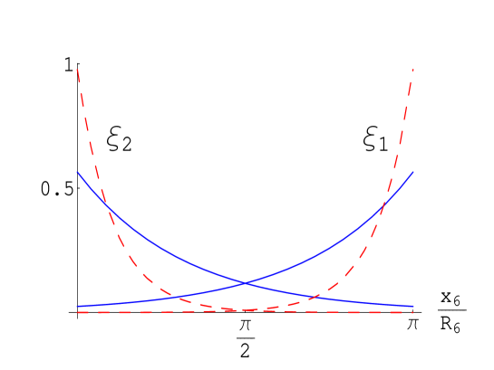
Figure 2: Wave functions $\xi^{(\alpha)}_{1,2}(x_{5},x_{6})$, in units of $\sqrt{R_{5}R_{6}}$. They have been obtained by choosing $|\mu_{(\alpha)}|R_{6}=1(3)$ for continuous-blue (dashed-red) lines.

Indeed, the zero mode proportional to $f^{(\alpha)}_{2}$ is localized at $x_{6}=0$ (mod $2\pi R_{6}$), whereas that proportional to $f^{(\alpha)}_{1}$ is peaked around $x_{6}=\pi R_{6}$ (mod $2\pi R_{6}$) (see figure 2). The two zero modes with well-defined localization properties in the compact space have non-trivial components both along $\eta$ and along $\chi$ and they are orthogonal to each other. The constant factors in eqs. (25) normalize the zero modes to 1. In our toy model, the number of zero modes is not related to a non-trivial topological property of the background $\epsilon(x_{6})$. The two zero modes are determined by the orbifold projection. The presence of the background only induces a separation of the corresponding wave functions in the compact space. Actually we can go smoothly from localized to constant wave functions, by turning off the constants $\mu_{(\alpha)}$, as apparent from eqs. (25).

With the introduction of the background, we now have two fermion generations, one sat at $x_{6}=0$ and the other at $x_{6}=\pi R_{6}$. From the point of view of the four-dimensional observer, who cannot resolve distances in the extra space, there is still a maximal flavour symmetry and, indeed, all fermions are still massless at this level. Fermions can acquire masses in the usual way, by breaking the electroweak symmetry via the non-vanishing VEV of a Higgs doublet $H$. If such a VEV were a constant in $x_{6}$, then we would obtain equal masses for the two fermion generations. Thus, to break the 4D flavour symmetry we need a non-trivial dependence of the Higgs VEV upon $x_{6}$. There are several ways to achieve this. For instance, we might assume that $H$ is a bulk field. Under certain conditions it may happen that the minimum of the energy is no longer $x_{6}$-constant. Examples of this kind are well-known in the literature [26]. If $H$ interacts with a suitable $x_{6}$-dependent background, there is a competition between the kinetic energy term, which prefers constant configurations, and the potential energy term, which may favour a $x_{6}$-varying VEV. In non-vanishing portions of the parameter space the minimum of the energy can depend non-trivially on $x_{6}$. In the minimal version of our toy model we will simulate this dependence in the simplest possible way, by introducing a Higgs doublet $H$ with hypercharge +1/2 localized along the line $x_{6}=0$ . The most general Yukawa interaction term invariant under $Z_{2}$, 6D parity and SU(3) $\otimes$ SU(2) $\otimes$ U(1) reads:

$${\cal L}_{Y}=\left[y_{u}~{}\tilde{H}^{\dagger}~{}\overline{\Psi^{(2)}}\Psi^{(1)}+y_{d}~{}H^{\dagger}~{}\overline{\Psi^{(3)}}\Psi^{(1)}+y_{e}~{}H^{\dagger}~{}\overline{\Psi^{(5)}}\Psi^{(4)}+h.c.\right]\delta(x_{6})~{}~{}~{},$$ (26)

where $\tilde{H}=i\sigma^{2}H^{*}$. Notice that $H$ has dimension +3/2 and $y$ has dimension -3/2, in mass units. In the next section we will see how a realistic pattern of masses and mixing angles arises from these Yukawa interactions.

Summarizing, our model is described by the Lagrangian:

$${\cal L}={\cal L}_{g}+{\cal L}_{m}+{\cal L}_{Y}+{\cal L}_{H}~{}~{}~{},$$ (27)

where ${\cal L}_{g}$, ${\cal L}_{m}$, ${\cal L}_{Y}$ are given in eqs. (1), (2) and (26), respectively, while ${\cal L}_{H}$, localized at $x_{6}=0$, contains the kinetic term for the Higgs doublet and the scalar potential that breaks spontaneously SU(2)$\otimes$U(1). The complex phases in $y$ can be completely eliminated via field redefinitions: in the limit of exact 6D parity symmetry all parameters are real.

3. Masses and Mixing Angles

The fermion mass terms arise from ${\cal L}_{Y}$ after electroweak symmetry breaking, here described by $\langle H\rangle=(0~{}v/\sqrt{2})^{T}$. To evaluate the fermion mass matrices we should expand the 6D fermion fields in 4D modes and then perform the $x_{5}$ and $x_{6}$ integrations. In practice, if we focus on the lightest sector, we can keep only the zero modes in the expansion. We obtain:

$$m_{u} = \frac{y_{u}}{\sqrt{2}}~{}v~{}\frac{\sqrt{|\mu_{(1)}\mu_{(2)}|}}{2\sqrt{(1-\lambda_{1}^{2})(1-\lambda_{2}^{2})}}\left(\begin{array}[]{cc}c_{u-}~{}\lambda_{1}\lambda_{2}&c_{u+}~{}\lambda_{2}\\ c_{u+}~{}\lambda_{1}&c_{u-}\end{array}\right)$$ (30)

$$m_{d} = \frac{y_{d}}{\sqrt{2}}~{}v~{}\frac{\sqrt{|\mu_{(1)}\mu_{(3)}|}}{2\sqrt{(1-\lambda_{1}^{2})(1-\lambda_{3}^{2})}}\left(\begin{array}[]{cc}c_{d-}~{}\lambda_{1}\lambda_{3}&c_{d+}~{}\lambda_{3}\\ c_{d+}~{}\lambda_{1}&c_{d-}\end{array}\right)$$ (33)

$$m_{e} = \frac{y_{e}}{\sqrt{2}}~{}v~{}\frac{\sqrt{|\mu_{(4)}\mu_{(5)}|}}{2\sqrt{(1-\lambda_{4}^{2})(1-\lambda_{5}^{2})}}\left(\begin{array}[]{cc}c_{e-}~{}\lambda_{4}\lambda_{5}&c_{e+}~{}\lambda_{5}\\ c_{e+}~{}\lambda_{4}&c_{e-}\end{array}\right)~{}~{}~{},$$ (36)

where

$$c_{u\pm}=1\pm\frac{\mu_{(1)}\mu_{(2)}}{|\mu_{(1)}\mu_{(2)}|}~{}~{}~{},~{}~{}~{}~{}~{}c_{d\pm}=1\pm\frac{\mu_{(1)}\mu_{(3)}}{|\mu_{(1)}\mu_{(3)}|}~{}~{}~{},~{}~{}~{}~{}~{}c_{e\pm}=1\pm\frac{\mu_{(4)}\mu_{(5)}}{|\mu_{(4)}\mu_{(5)}|}~{}~{}~{},$$ (37)

and

$$\lambda_{\alpha}=e^{\displaystyle{-\pi|\mu_{(\alpha)}|R_{6}}}~{}~{}~{}.$$ (38)

These mass matrices, here given in the convention $\overline{f_{R}}m_{f}f_{L}$, are not hermitian. It is interesting to see that, for generic order-one values of the dimensionless combinations $c_{f\pm}$ and $\mu_{(\alpha)}R_{6}$, the mass matrices display a clear hierarchical pattern. Fermion masses of the first generation are suppressed by $\lambda_{(\alpha)}\lambda_{(\beta)}$ compared to those of the second generation and mixing angles are of order $\lambda_{(\alpha)}$ or $\lambda_{(\beta)}$. This is quite similar to what obtained in 4D models with a spontaneously broken flavour symmetry. Here the role of small expansion parameters is played by the quantities $\lambda_{\alpha}$. However in our parity invariant model, the parameters $\mu_{(\alpha)}$ are real and the coefficients $c_{f\pm}$ are ‘quantized’. Either $c_{f+}$ or $c_{f-}$ should vanish and this implies no mixing. Indeed when 6D parity is conserved, we have only two possible orientations of the fermionic zero modes in the $(\eta,\chi)$ space: either $(1,i)$ or $(1,-i)$, as apparent from eqs. (14) and (24). Thus the scalar product between two zero modes in the $(\eta,\chi)$ space is either maximal or zero. Modulo a relabelling among first and second generations, this gives rise to a perfect alignment of mass matrices and a vanishing overall mixing. To overcome this problem, we should relax the assumption of exact 6D parity symmetry . We will assume that 6D parity is broken ‘softly’, by the fermion-background interaction described by ${\cal L}_{m}$. This can be achieved by taking complex values for the mass coefficients $\mu_{(\alpha)}$ . In a fundamental theory such a breaking could be spontaneous: if $m_{(\alpha)}$ were complex fields, then the Lagrangian would still be invariant under 6D parity acting as $m_{(\alpha)}\leftrightarrow m_{(\alpha)}^{\dagger}$. It might occur that the dynamics of the fields $m_{(\alpha)}$ led to complex VEVs for $m_{(\alpha)}$, thus spontaneously breaking parity. In our toy model we will simply assume the existence of such a complex background. All the relations that we have derived hold true for the complex case as well and we have now hierarchical mass matrices with a non-trivial intergenerational mixing. By expanding the results at leading order in $\lambda_{\alpha}$ we find:

$$m_{c}=|y_{u}|v\frac{\sqrt{|\mu_{(1)}\mu_{(2)}|}}{2\sqrt{2}}|c_{u-}|~{}~{}~{}~{}~{}~{}m_{s}=|y_{d}|v\frac{\sqrt{|\mu_{(1)}\mu_{(3)}|}}{2\sqrt{2}}|c_{d-}|~{}~{}~{}~{}~{}~{}m_{\mu}=|y_{e}|v\frac{\sqrt{|\mu_{(4)}\mu_{(5)}|}}{2\sqrt{2}}|c_{e-}|~{}~{},$$ (39)

and

$$\frac{m_{u}}{m_{c}}=\frac{|c_{u+}^{2}-c_{u-}^{2}|}{|c_{u-}|^{2}}\lambda_{1}\lambda_{2}~{}~{}~{}~{}~{}\frac{m_{d}}{m_{s}}=\frac{|c_{d+}^{2}-c_{d-}^{2}|}{|c_{d-}|^{2}}\lambda_{1}\lambda_{3}~{}~{}~{}~{}~{}\frac{m_{e}}{m_{\mu}}=\frac{|c_{e+}^{2}-c_{e-}^{2}|}{|c_{e-}|^{2}}\lambda_{4}\lambda_{5}~{}~{}~{}.$$ (40)

Finally, after absorbing residual phases in the definition of the $s$ and $c$ 4D fields, the matrices $m_{u}^{\dagger}m_{u}$ and $m_{d}^{\dagger}m_{d}$ are diagonalized by orthogonal transformations characterized by mixing angles $\theta_{u,d}$:

$$\theta_{u,d}=\left|\frac{c_{u,d+}}{c_{u,d-}}\right|\lambda_{1}~{}~{}~{},$$ (41)

still at leading order in $\lambda_{\alpha}$. Therefore the Cabibbo angle is given by:

$$\theta_{C}=\left(\left|\frac{c_{d+}}{c_{d-}}\right|-\left|\frac{c_{u+}}{c_{u-}}\right|\right)\lambda_{1}~{}~{}~{}.$$ (42)

Barring accidental cancellations in the relevant combinations of the coefficients $c_{f\pm}$, the Cabibbo angle is of order $\lambda_{1}$. Then, by assuming $\lambda_{3}\approx\lambda_{1}$ and $\lambda_{2}\approx\lambda_{1}^{3}$ we reproduce the correct order of magnitude of mass ratios in the quark sector. These are small numbers in the 4D theory, but can be obtained quite naturally from the 6D point of view: $\mu_{(1)}R_{6}\approx\mu_{(3)}R_{6}\approx 0.5$ and $\mu_{(2)}R_{6}\approx 1.3$. Similarly, by taking $\lambda_{4}\lambda_{5}\approx\lambda_{1}^{2}$ we can naturally fit the lepton mass ratio.

It can be useful to comment about the way flavour symmetry is broken in this toy model. Before the introduction of the Yukawa interactions and modulo U(1) anomalies, the flavour symmetry group is U(2)⁵. After turning the Yukawa couplings on, we can consider several limits. When $R_{6}\to\infty$, the quantities $\lambda_{(\alpha)}$ vanish and the flavour symmetry is broken down to U(1)⁵, acting non-trivially on the lightest sector. If $R_{6}$ is finite and non-vanishing, U(1)⁵ is in turn completely broken down by $\lambda_{(\alpha)}\neq 0$. Nevertheless, contrary to what happens in models with abelian flavour symmetries, the coefficients of order one that multiply the symmetry breaking parameters $\lambda_{(\alpha)}$ are now related one to each other. This can be appreciated by taking the limit $R_{6}\to 0$. We have $\lambda_{(\alpha)}=1$ and the residual flavour symmetry is a permutation symmetry, separately for the lepton and the quark sectors: $S_{2}\otimes S_{2}$.

Let us now briefly comment about neutrino masses and mixings in this set-up. The most straightforward way to produce neutrino masses is to add a gauge singlet 6D fermion field, $\Psi^{(6)}$, with $Z_{2}$ assignments $(+1,-1,-1,+1)$. As for the case of charged fermions, by introducing a mass term for $\Psi^{(6)}$ as in eq. (2) and a Yukawa interaction with $\Psi^{(4)}$ and $\tilde{H}$ as in eq. (26), we obtain a Dirac neutrino mass term

$$m_{\nu}=\frac{y_{\nu}}{\sqrt{2}}v\frac{\sqrt{|\mu_{(4)}\mu_{(6)}|}}{2\sqrt{(1-\lambda_{4}^{2})(1-\lambda_{6}^{2})}}\left(\matrix{c_{\nu-}\lambda_{4}\lambda_{6}&c_{\nu+}\lambda_{6}\cr c_{\nu+}\lambda_{4}&c_{\nu-}}\right)$$ (43)

A large mixing angle in the leptonic sector, $\theta_{L}$, is obtained for $\lambda_{4}=O(1)$, in which case the neutrino mass hierarchy,

$$\frac{m_{\nu_{1}}}{m_{\nu_{2}}}=\frac{|c_{\nu+}^{2}-c_{\nu-}^{2}|}{|c_{\nu-}|^{2}}\lambda_{4}\lambda_{6}~{}~{}~{},$$ (44)

is controlled by $\lambda_{6}$. At leading order, the left mixings in $m_{e}^{\dagger}m_{e}$ and $m_{\nu}^{\dagger}m_{\nu}$ correspond to

$$\tan 2\theta_{e,\nu}=\frac{2~{}c_{e,\nu+}~{}c_{e,\nu-}~{}\lambda_{4}}{(c_{e,\nu-}^{2}-c_{e,\nu+}^{2}~{}\lambda_{4}^{2})}~{}~{}~{},$$ (45)

so that $\theta_{L}\equiv\theta_{\nu}-\theta_{e}$ is naturally large. As in 4D, the smallness of these Dirac neutrino masses with respect to the electroweak scale has to be imposed by an ad hoc suppression of the Yukawa couplings $y_{\nu}$. A natural suppression could be achieved by considering also a Majorana mass term in the bulk for the field $\Psi^{(6)}$. Alternatively, one could write localized Majorana mass terms directly on the 4D brane or even exploit a seventh warped extra-dimension [27].

4. Which scale for flavour physics?

Our 6D toy model is non renormalizable. It is characterized by some typical mass scale $\Lambda$. At energies larger than this typical scale, the description offered by the model is not accurate enough and some other theory should replace it. Up to now we have not specified $\Lambda$. We could have in mind a traditional picture where $\Lambda$ is very large, perhaps close to the 4D Planck scale, where presumably all particle interactions, including the gravitational one, are unified in a fundamental theory. In this scenario we have the usual hierarchy problem. Clearly our simple model cannot explain why $v<<\Lambda^{3/2}$ and we should rely on some additional mechanism to render the electroweak breaking scale much smaller compared to $\Lambda$. A supersymmetric or warped version of our toy model could alleviate the technical aspect of the hierarchy problem. Alternatively, we could ask how small could $\Lambda$ be without producing a conflict with experimental data. For simplicity we assume that the two radii $R_{5}$, $R_{6}$ are approximately of the same order $R$. Due to the different dimension between 6D and 4D fields, coupling constants of the effective 4D theory are suppressed by volume factors and we require $\Lambda R\geq 1$ to work in a weakly coupled regime. Therefore, lower bounds on $1/R$ are also lower bounds for $\Lambda$. Lower bounds on $1/R$ come from the search of the first Kaluza-Klein modes at the existing colliders or from indirect effects induced by the additional heavy modes [8, 9, 28, 29]. These last effects lead to departures from the SM predictions in electroweak observables. From the precision tests of the electroweak sector, we get a lower bound on $1/R$ in the $TeV$ range. However, the most dangerous indirect effects are those leading to violations of universality in gauge interactions and those contributing to flavour changing processes. Indeed, whenever we have a source of flavour symmetry breaking, we expect a violation of universality at some level. In the SM such violation comes through loop effects from the Yukawa couplings and it is tiny. In our model, as we will see, such effects can already arise at tree level and, to respect the experimental bounds, a sufficiently large scale $1/R$ is needed [30].

Since in each fermion sector the two generations are described by two copies of the same wave function, differing only in their localization along $x_{6}$, the universality of the gauge interactions will be guaranteed if the gauge vector bosons have a wave function perfectly constant in $x_{6}$. This is the case only for massless gauge vector bosons, such as the photon, but, as we will see now, not necessarily for the massive gauge vector bosons like $W$ and $Z$. Moreover, also the higher Kaluza-Klein modes of all gauge bosons have non-constant wave functions and their interactions with split fermions are in general non-universal.

We start by discussing the interactions between the lightest fermion generations and the observed $W$ and $Z$ vector bosons. Consider, for simplicity, the limit of vanishing gauge coupling $g^{\prime}$ for $U(1)$. Then the free equation of motion for the gauge bosons $W_{\mu}$ of $SU(2)$ reads:

$$\Box W_{\mu}+\frac{g^{2}}{2}h^{2}(x_{6})W_{\mu}=0~{}~{}~{},$$ (46)

where $h(x_{6})$ denotes the $x_{6}$-dependent VEV of the Higgs doublet $H$. To avoid problems in dealing with singular, ill-defined functions, here $h(x_{6})$ is a smooth function, VEV of a 6D bulk field. From the eq. (46) we will see that, if $h(x_{6})$ is not constant, then the lightest mode for the gauge vector bosons is no longer described by a constant wave function. Therefore the 4D gauge interactions, resulting from the overlap of fermion and vector bosons wave functions, can be different for the two generations.

In general we are not able to solve the above equation exactly, but we can do this by a perturbative expansion in $g^{2}$, which we could justify a posteriori. At zeroth order the $W^{3}$ mass and the corresponding wave function are given by:

$$(m^{(0)}_{W})^{2}=0~{}~{}~{}~{}~{}~{}~{}~{}~{}~{}~{}~{}~{}W^{(0)}_{\mu}=\frac{1}{\sqrt{2\pi^{2}R_{5}R_{6}}}~{}~{}~{}.$$ (47)

At first order we find:

$$m_{W}^{2} = \frac{g^{2}}{2\pi R_{6}}\int_{0}^{+\pi R_{6}}dx_{6}~{}h^{2}(x_{6})$$

$$W_{\mu} = W^{(0)}_{\mu}(1+\delta W_{\mu}(x_{6}))$$

$$\delta W_{\mu}(x_{6}) = \int_{0}^{x_{6}}du\int_{0}^{u}dz(\frac{g^{2}}{2}h^{2}(z)-m_{W}^{2})~{}~{}~{},$$ (48)

modulo an arbitrary additive constant in $W_{\mu}$, that can be adjusted by normalization. We see that when $h(x_{6})$ is constant, the usual result is reproduced: $m_{W}^{2}=g^{2}h^{2}/2$ and the corresponding wave function does not depend on $x_{6}$. Eq. (48) allows us to compute the fractional difference $(g_{1}-g_{2})/(g_{1}+g_{2})$ between the SU(2) couplings to the first and second fermion generation, respectively. Focusing on $W^{3}_{\mu}$, we obtain:

$$\left|\frac{g_{1}-g_{2}}{g_{1}+g_{2}}\right|=\frac{\int_{0}^{\pi R_{6}}dx_{6}~{}\left(|\xi^{(\alpha)}_{1}|^{2}-|\xi^{(\alpha)}_{2}|^{2}\right)\delta W^{3}_{\mu}}{\int_{0}^{\pi R_{6}}dx_{6}~{}\left(|\xi^{(\alpha)}_{1}|^{2}+|\xi^{(\alpha)}_{2}|^{2}\right)}~{}~{}~{},$$ (49)

where $\alpha=1,4$. As expected, if $\delta W^{3}_{\mu}$ is $x_{6}$-constant, then the gauge couplings are universal. From the precision tests of the SM performed in the last decade at LEP and SLC we expect that such a difference should not exceed, say, the per-mill level. We have analyzed numerically eq. (49) for several choices of the parameters and for several possible profiles of the VEV $h(x_{6})$. We found that universality is respected at the per-mill level for $m_{W}^{2}R_{6}^{2}<O(10^{-3})$ or $1/R_{6}>3~{}TeV$.

Much more severe are the bounds associated to the interactions of the higher modes arising from the Kaluza-Klein decomposition of the gauge vector bosons:

$$A_{\mu}=i\sum_{c,m,n}t^{c}A_{\mu}^{c(m,n)}(x)z_{mn}(x_{5},x_{6})~{}~{}~{},$$ (50)

where $t^{c}$ are the generators of the gauge group factor, $A_{\mu}^{c(m,n)}(x)$ the corresponding 4D vector bosons and $z_{mn}(x_{5},x_{6})$ the periodic, $Z_{2}$-even wave functions:

$$z_{mn}(x_{5},x_{6})=\frac{1}{\sqrt{\pi^{2}R_{5}R_{6}2^{\delta_{m,0}\delta_{n,0}}}}\cos(m\frac{x_{5}}{R_{5}}+n\frac{x_{6}}{R_{6}})~{}~{}~{}.$$ (51)

In eq. (50) $m$ and $n\geq 0$ are integers: $m$ runs from $-\infty$ to $+\infty$ for positive $n$ and from $0$ to $+\infty$ for $n=0$. From eq. (1) we obtain the 4D interaction term:

$$-\frac{g}{\Lambda}\sum_{a,b}\sum_{m,n}c_{ab}^{mn}~{}\overline{f^{(\alpha)}_{a}(x)}~{}\gamma^{\mu}t^{c}~{}f^{(\alpha)}_{b}(x)~{}A_{\mu}^{c(m,n)}(x)~{}~{}~{},$$ (52)

where $g$ denotes the gauge coupling constant of the relevant group factor and the scale $\Lambda$ has been included to make $g$ dimensionless. The coefficients $c_{ab}^{mn}$ $(a,b=1,2)$ describe the overlap among the fermion and gauge-boson wave functions. We obtain:

$$c_{ab}^{mn} = 0~{}~{}~{}~{}~{}~{}~{}~{}~{}~{}m\neq 0$$

$$c_{ab}^{0n} = 0~{}~{}~{}~{}~{}~{}~{}~{}~{}~{}a\neq b$$

$$c_{11}^{0n} = \frac{1}{\sqrt{\pi^{2}R_{5}R_{6}2^{\delta_{n,0}}}}\frac{4|\mu_{\alpha}|^{2}R_{6}^{2}}{n^{2}+4|\mu_{\alpha}|^{2}R_{6}^{2}}\frac{(1-(-1)^{n}e^{2|\mu_{\alpha}|\pi R_{6}})}{(1-e^{2|\mu_{\alpha}|\pi R_{6}})}$$

$$c_{22}^{0n} = (-1)^{n}c_{11}^{0n}$$ (53)

For odd $n$, the interactions mediated by $A_{\mu}^{c(0,n)}$ are non-universal. By asking that universality holds within the experimental limits, we get a lower bound on $1/R$ similar to that discussed before, of the order of some $TeV$. However, stronger bounds are obtained from the interactions in eqs. (52,53), by considering their contribution to flavour changing processes. Indeed, after electroweak symmetry breaking, we should account for the unitary transformations bringing fermions from the interaction basis to the mass eigenstate basis. The terms involving $A_{\mu}^{c(0,2n+1)}$ are not invariant under such transformations and flavour changing interactions are produced. By integrating out the heavy modes $A_{\mu}^{c(0,2n+1)}$ we obtain an effective, low-energy description of flavour violation in terms of four-fermion operators, suppressed by the square of the compactification scale, $(1/R_{6})^{2}$. The most relevant effects of these operators have been discussed by Delgado, Pomarol and Quiros in ref. [31] in a context which is very close to the one we are considering here. By analyzing the contribution to $\Delta m_{K}$ and to $\epsilon_{K}$, these authors derived a lower bound on $1/R$ of $O(100~{}TeV)$ and of $O(1000~{}TeV)$, respectively, which at least as an order of magnitude applies also to our model.

5. Outlook

We have presented and analyzed a model for flavour in two extra dimensions. For each irreducible representation of the SM, there is a single, vector-like 6D fermion. Four dimensional fermion generations arise from orbifold projection in the compactification mechanism. In the toy model discussed here there is only room for two generations and a natural question is whether this approach can be generalized to the realistic case of three generations. The obvious objection is that the number of 4D components of a higher dimensional fermion is a power of two. In principle, an odd number of massless modes can be obtained by eliminating some of the unwanted components via orbifold projection and/or non-periodic boundary conditions. In our model flavour symmetry is broken in two steps. First, the independent zero modes are localized at different points along the sixth dimension by means of a generalized 6D mass term, described by a scalar background. Our background is topologically trivial and does not modify the number of zero modes, which is fixed by the orbifold projection. However, the presence of a background with a non-trivial topology may change the number of chiral zero modes, thus contributing to reproduce the realistic case [22, 23]. The flavour symmetry is then broken by turning on standard Yukawa interaction with a Higgs field developing a non-constant VEV. In the model explored here the geometry of the compact space is the simplest one and it is essentially one dimensional. The generations are localized along the sixth dimension, and the fifth dimension does not play any active role. In a more realistic model it might be necessary to fully exploit the geometry of the compact space, in order to obtain a successful arrangement for the zero modes. A specific problem is represented by the neutrino sector, that we have only briefly touched here. Another unpleasant feature of our toy model is that, despite its simplicity, it contains too many parameters and there are no testable predictions. Clearly the issue of predictability is crucial for a realistic model. It is possible that, by going to the realistic case of three generations, the number of parameters does not increase, thus allowing for quantitative tests of this approach. Alternatively, we could consider more constrained frameworks. A possibility could be to exploit a grand unification symmetry to limit the number of parameters in the fermion sector. Another interesting case is represented by theories where the Higgs fields are identified with the extra components of higher dimensional gauge vector bosons [32]. One of the main problems of these models is precisely to break flavour symmetry, starting from universal Yukawa couplings, universality being dictated by gauge invariance [33]. Our approach could provide a possible mechanism to realize such breaking.

Despite the fact that our model is incomplete in many respects, we think that it possesses several interesting theoretical properties. At variance with most of the existing 4D models, the problem of flavour symmetry breaking is here tightly related to the problem of obtaining the right number of generations. Starting from dimensionless parameters of order one, we were able to obtain a hierarchical pattern of masses. They are described by mass matrices that are very close in structure to those obtained in 4D models by enforcing abelian flavour symmetries, and provide a successful description of both quark and lepton spectra. The crucial difference is that, whereas in the 4D case, the order-one coefficients multiplying powers of the symmetry breaking parameters are completely undetermined, in our case those coefficients are strongly correlated and predictable in terms of the underlying parameters. We have also a quite non-standard interpretation of the intergenerational mixing, that appears to be related to a soft breaking of 6D parity symmetry. Starting from vector-like 6D fermions transforming as a SM generation, we automatically obtain cancellation of bulk and localized gauge anomalies, a rather non-trivial result in 6D gauge theories. Hopefully some of these features could also become part of a more realistic framework.

Acknowledgements. We thank Guido Altarelli, Riccardo Barbieri, Augusto Sagnotti, Jose Santiago and Angel Uranga for valuable discussions. C.B., F.F. and I.M. thank the CERN theoretical division for hospitality in summer/fall 2002, when we began the present work. This project is partially supported by the European Programs HPRN-CT-2000-00148 and HPRN-CT-2000-00149.

Appendix

$\Gamma$ matrices

We work with the metric

$$\eta_{MN}=\textrm{diag}(1,-1,-1,-1,-1,-1)$$ (54)

where $M,N=0,1,2,3,5,6$. The representation of 6D $\Gamma$-matrices we use in the text is

$$\Gamma^{\mu}=\left(\begin{array}[]{cc}\gamma^{\mu}&0\\ 0&\gamma^{\mu}\end{array}\right)\ ,\ \ \Gamma^{5}=i\ \left(\begin{array}[]{cc}0&\gamma_{5}\\ \gamma_{5}&0\end{array}\right)\ ,\ \ \Gamma^{6}=i\ \left(\begin{array}[]{cc}0&i\ \gamma_{5}\\ -i\ \gamma_{5}&0\end{array}\right)\ ,$$ (55)

with $\mu=0,1,2,3$. Here $\gamma^{\mu}$, $\gamma_{5}$ are 4D $\gamma$-matrices given by

$$\gamma^{0}=\left(\begin{array}[]{cc}\mathbf{1}&0\\ 0&\mathbf{-1}\end{array}\right)\ ,\ \ \gamma^{i}=\left(\begin{array}[]{cc}0&\sigma^{i}\\ -\sigma^{i}&0\end{array}\right)\ ,\ \ \gamma^{5}=\left(\begin{array}[]{cc}0&\mathbf{1}\\ \mathbf{1}&0\end{array}\right)\ ,$$ (56)

where $\sigma^{i}$ are the Pauli matrices.

In 6D the analogous of $\gamma_{5}$, $\Gamma_{7}\ (=\Gamma^{7})$, is defined by:

$$\Gamma_{7}=\Gamma_{0}\Gamma_{1}\Gamma_{2}\Gamma_{3}\Gamma_{5}\Gamma_{6}=\left(\begin{array}[]{cc}\gamma^{5}&0\\ 0&-\gamma^{5}\end{array}\right)\ .$$ (57)

Localization of zero modes

Starting from eqs. (4), we obtain the following second order partial differential equations, holding in the whole $(x_{5},x_{6})$ plane:

$$(\partial_{5}^{2}+\partial_{6}^{2})\ \chi_{L}^{\alpha}-|\mu_{(\alpha)}|^{2}\ \epsilon^{2}(x_{6})\ \chi_{L}^{\alpha}-2\ i\ \mu_{(\alpha)}\ (-1)^{k}\ \delta_{k}(x_{6})\ \eta_{L}^{\alpha} = 0$$

$$(\partial_{5}^{2}+\partial_{6}^{2})\ \eta_{L}^{\alpha}-|\mu_{(\alpha)}|^{2}\ \epsilon^{2}(x_{6})\ \eta_{L}^{\alpha}+2\ i\ \mu_{(\alpha)}^{*}\ (-1)^{k}\ \delta_{k}(x_{6})\ \chi_{L}^{\alpha} = 0$$

$$(\partial_{5}^{2}+\partial_{6}^{2})\ \chi_{R}^{\alpha}-|\mu_{(\alpha)}|^{2}\ \epsilon^{2}(x_{6})\ \chi_{R}^{\alpha}+2\ i\ \mu_{(\alpha)}^{*}\ (-1)^{k}\ \delta_{k}(x_{6})\ \eta_{R}^{\alpha} = 0$$

$$(\partial_{5}^{2}+\partial_{6}^{2})\ \eta_{R}^{\alpha}-|\mu_{(\alpha)}|^{2}\ \epsilon^{2}(x_{6})\ \eta_{R}^{\alpha}-2\ i\ \mu_{(\alpha)}\ (-1)^{k}\ \delta_{k}(x_{6})\ \chi_{R}^{\alpha} = 0$$ (58)

where $k$ is an integer, $\delta_{k}(x_{6})\equiv\delta(x_{6}-k\pi R_{6})$ and the sum over $k$ is understood. In the bulk these equations are decoupled and identical for all fields. Away from the lines $x_{6}=k\pi R_{6}$ $k\in Z$, they read:

$$(\partial_{5}^{2}+\partial_{6}^{2})\ \phi-|\mu_{(\alpha)}|^{2}\ \phi=0$$ (59)

with appropriate boundary conditions. Here $\phi$ stands for $\chi_{L}^{\alpha}$, $\eta_{L}^{\alpha}$, $\chi_{R}^{\alpha}$, $\eta_{R}^{\alpha}$. In each strip $k\pi R_{6}<x_{6}<(k+1)\pi R_{6}$, the general solution to this equation can be written in the form:

$$\phi^{(k)}(x,x_{5},x_{6})=\sum_{n\in Z}\ \left[\ C^{(k)}_{n}(x)\ e^{\displaystyle\alpha_{n}\frac{x_{6}}{R_{5}}}+C^{\prime(k)}_{n}(x)\ e^{\displaystyle-\alpha_{n}\frac{x_{6}}{R_{5}}}\ \right]\ e^{\displaystyle in\frac{x_{5}}{R_{5}}}$$ (60)

with $\alpha_{n}=\sqrt{n^{2}+|\mu_{\alpha}|^{2}R_{5}^{2}}$. These solutions can be glued together by imposing periodicity along $x_{6}$, $Z_{2}$ parity and the appropriate discontinuity across the lines $x_{6}=k\pi R_{6}$. This last requirement can be directly derived from eqs. (4) and eqs. (58). The fields $\phi$ should be continuous everywhere, whereas their first derivatives have discontinuities $\Delta^{(k)}(\partial_{6}\phi)$ given by:

$$\begin{array}[]{ll}\Delta^{(2k)}(\partial_{6}\phi)=-2\,i\,s(\phi^{\prime})\,\phi^{\prime}(2k\pi R_{6})&\textrm{at}\quad x_{6}=2k\pi R_{6}\\ \Delta^{(2k+1)}(\partial_{6}\phi)=2\,i\,s(\phi^{\prime})\,\phi^{\prime}((2k+1)\pi R_{6})&\textrm{at}\quad x_{6}=(2k+1)\pi R_{6}\end{array}$$ (61)

where $(\phi,\phi^{\prime})=(\chi_{L}^{\alpha},\eta_{L}^{\alpha}),\,(\eta_{L}^{\alpha},\chi_{L}^{\alpha}),\,(\chi_{R}^{\alpha},\eta_{R}^{\alpha}),\,(\eta_{R}^{\alpha},\chi_{R}^{\alpha})$ and

$$s(\phi^{\prime})=\left\{\begin{array}[]{ll}-\mu_{\alpha}&\textrm{if}\ \phi^{\prime}=\eta_{L}^{\alpha},\,\chi_{R}^{\alpha}\\ \mu_{\alpha}^{*}&\textrm{if}\ \phi^{\prime}=\eta_{R}^{\alpha},\,\chi_{L}^{\alpha}\end{array}\right..$$ (62)

Only for $n=0$ these requirements have a non-trivial solution. This means that the zero modes are independent of $x_{5}$. More precisely, $Z_{2}$-odd fields are identically vanishing, while for even fields we get:

$$\begin{array}[]{lcl}\eta^{\alpha}_{L,R}(x,x_{5},x_{6})&=&N^{(\alpha)}_{1}f^{(\alpha)}_{1}(x)\,e^{\displaystyle|\mu_{\alpha}|\,|x_{6}|_{per}}\\ &+&\,N^{(\alpha)}_{2}f^{(\alpha)}_{2}(x)\,e^{\displaystyle-|\mu_{\alpha}|\,|x_{6}|_{per}}\\[5.69046pt] \chi^{\alpha}_{L,R}(x,x_{5},x_{6})&=&i\,\displaystyle\frac{s^{*}(\chi^{\alpha}_{L,R})}{|\mu_{\alpha}|}\,N^{(\alpha)}_{1}f^{(\alpha)}_{1}(x)\,e^{\displaystyle|\mu_{\alpha}|\,|x_{6}|_{per}}\\ &-&\,i\,\displaystyle\frac{s^{*}(\chi^{\alpha}_{L,R})}{|\mu_{\alpha}|}\,N^{(\alpha)}_{2}f^{(\alpha)}_{2}(x)\,e^{\displaystyle-|\mu_{\alpha}|\,|x_{6}|_{per}}\,,\end{array}$$ (63)

where $f^{(\alpha)}_{1,2}(x)$ are $x$-dependent spinors and $N^{(\alpha)}_{1,2}$ denote normalization constants, which are explicitly given in eq. (25) of the text.

References

- [1] K. Hagiwara et al. [Particle Data Group Collaboration], Phys. Rev. D 66 (2002) 010001.
- [2] G.L. Fogli talk at the X International Workshop on Neutrino Telescopes, March 11-14, 2003, Venice (Italy), [http://axpd24.pd.infn.it/conference2003/]; G. Altarelli and F. Feruglio, arXiv:hep-ph/0206077 and talks at the X International Workshop on Neutrino Telescopes, March 11-14, 2003, Venice (Italy), [http://axpd24.pd.infn.it/conference2003/].
- [3] C.D. Froggatt and H. B. Nielsen, Nucl. Phys. B 147 (1979) 277.
- [4] P. Candelas, G. T. Horowitz, A. Strominger and E. Witten, Nucl. Phys. B 258 (1985) 46.
- [5] L. J. Dixon, J. A. Harvey, C. Vafa and E. Witten, Nucl. Phys. B 261 (1985) 678 and Nucl. Phys. B 274 (1986) 285.
- [6] L. E. Ibanez, Phys. Lett. B 181 (1986) 269; S. Hamidi and C. Vafa, Nucl. Phys. B 279 (1987) 465; L. J. Dixon, D. Friedan, E. J. Martinec and S. H. Shenker, Nucl. Phys. B 282 (1987) 13.
- [7] See, for instance, D. Cremades, L. E. Ibanez and F. Marchesano, arXiv:hep-th/0302105 and references therein.
- [8] A. Pomarol and M. Quiros, Phys. Lett. B 438 (1998) 255 [arXiv:hep-ph/9806263]; M. Masip and A. Pomarol, Phys. Rev. D 60 (1999) 096005 [arXiv:hep-ph/9902467]; P. Nath and M. Yamaguchi, Phys. Rev. D 60 (1999) 116006 [arXiv:hep-ph/9903298]; P. Nath, Y. Yamada and M. Yamaguchi, Phys. Lett. B 466 (1999) 100 [arXiv:hep-ph/9905415]; R. Casalbuoni, S. De Curtis, D. Dominici and R. Gatto, Phys. Lett. B 462 (1999) 48 [arXiv:hep-ph/9907355]; T. Gherghetta and A. Pomarol, Nucl. Phys. B 586 (2000) 141 [arXiv:hep-ph/0003129]; N. Arkani-Hamed, L. J. Hall, Y. Nomura, D. R. Smith and N. Weiner, Nucl. Phys. B 605 (2001) 81 [arXiv:hep-ph/0102090]; A. Delgado and M. Quiros, Nucl. Phys. B 607 (2001) 99 [arXiv:hep-ph/0103058]; A. Delgado, G. von Gersdorff, P. John and M. Quiros, Phys. Lett. B 517 (2001) 445 [arXiv:hep-ph/0104112]; G. von Gersdorff, N. Irges and M. Quiros, Nucl. Phys. B 635 (2002) 127 [arXiv:hep-th/0204223]; G. von Gersdorff, N. Irges and M. Quiros, arXiv:hep-ph/0206029; C. Biggio and F. Feruglio, Annals Phys. 301 (2002) 65 [arXiv:hep-th/0207014]; M. Carena, T. M. Tait and C. E. Wagner, Acta Phys. Polon. B 33 (2002) 2355 [arXiv:hep-ph/0207056]; G. von Gersdorff, N. Irges and M. Quiros, Phys. Lett. B 551 (2003) 351 [arXiv:hep-ph/0210134]; F. del Aguila, M. Perez-Victoria and J. Santiago, JHEP 0302 (2003) 051 [arXiv:hep-th/0302023].
- [9] T. Appelquist and H. U. Yee, Phys. Rev. D 67 (2003) 055002 [arXiv:hep-ph/0211023]; T. Appelquist, B. A. Dobrescu, E. Ponton and H. U. Yee, Phys. Rev. D 65 (2002) 105019 [arXiv:hep-ph/0201131]; T. Appelquist, B. A. Dobrescu, E. Ponton and H. U. Yee, Phys. Rev. Lett. 87 (2001) 181802 [arXiv:hep-ph/0107056]; T. Appelquist and B. A. Dobrescu, Phys. Lett. B 516 (2001) 85 [arXiv:hep-ph/0106140]; T. Appelquist, H. C. Cheng and B. A. Dobrescu, Phys. Rev. D 64 (2001) 035002 [arXiv:hep-ph/0012100].
- [10] J. Scherk and J. H. Schwarz, Nucl. Phys. B 153 (1979) 61 and Phys. Lett. B 82 (1979) 60; P. Fayet, Phys. Lett. B 159 (1985) 121 and Nucl. Phys. B 263 (1986) 649.
- [11] I. Antoniadis, S. Dimopoulos, A. Pomarol and M. Quiros, Nucl. Phys. B 544 (1999) 503 [arXiv:hep-ph/9810410]; A. Delgado, A. Pomarol and M. Quiros, Phys. Rev. D 60 (1999) 095008 [arXiv:hep-ph/9812489]; D. E. Kaplan, G. D. Kribs and M. Schmaltz, Phys. Rev. D 62 (2000) 035010 [arXiv:hep-ph/9911293]; R. Barbieri, L. J. Hall and Y. Nomura, Phys. Rev. D 63 (2001) 105007 [arXiv:hep-ph/0011311]; T. Gherghetta and A. Pomarol, Nucl. Phys. B 602 (2001) 3 [arXiv:hep-ph/0012378]; D. Marti and A. Pomarol, Phys. Rev. D 64 (2001) 105025 [arXiv:hep-th/0106256]; R. Barbieri, L. J. Hall and Y. Nomura, Nucl. Phys. B 624 (2002) 63 [arXiv:hep-th/0107004]; J. A. Bagger, F. Feruglio and F. Zwirner, Phys. Rev. Lett. 88 (2002) 101601 [arXiv:hep-th/0107128]; A. Masiero, C. A. Scrucca, M. Serone and L. Silvestrini, Phys. Rev. Lett. 87 (2001) 251601 [arXiv:hep-ph/0107201]; R. Barbieri, L. J. Hall and Y. Nomura, arXiv:hep-ph/0110102; G. von Gersdorff, M. Quiros and A. Riotto, Nucl. Phys. B 634 (2002) 90 [arXiv:hep-th/0204041]; V. Di Clemente, S. F. King and D. A. Rayner, Nucl. Phys. B 646 (2002) 24 [arXiv:hep-ph/0205010]; D. Marti and A. Pomarol, Phys. Rev. D 66 (2002) 125005 [arXiv:hep-ph/0205034]; R. Barbieri, G. Marandella and M. Papucci, Phys. Rev. D 66 (2002) 095003 [arXiv:hep-ph/0205280]; R. Barbieri, L. J. Hall, G. Marandella, Y. Nomura, T. Okui, S. J. Oliver and M. Papucci, arXiv:hep-ph/0208153; C. Biggio, F. Feruglio, A. Wulzer and F. Zwirner, JHEP 0211 (2002) 013 [arXiv:hep-th/0209046]; A. Delgado, G. von Gersdorff and M. Quiros, JHEP 0212 (2002) 002 [arXiv:hep-th/0210181]; L. J. Hall, Y. Nomura, T. Okui and S. J. Oliver, arXiv:hep-th/0302192.
- [12] Y. Hosotani, Phys. Lett. B 126 (1983) 309 and Annals Phys. 190 (1989) 233.
- [13] Y. Kawamura, Prog. Theor. Phys. 105 (2001) 999 [arXiv:hep-ph/0012125]; G. Altarelli and F. Feruglio, Phys. Lett. B 511 (2001) 257 [arXiv:hep-ph/0102301]; L. J. Hall and Y. Nomura, Phys. Rev. D 64 (2001) 055003 [arXiv:hep-ph/0103125]; A. Hebecker and J. March-Russell, Nucl. Phys. B 613 (2001) 3 [arXiv:hep-ph/0106166]; R. Barbieri, L. J. Hall and Y. Nomura, Phys. Rev. D 66 (2002) 045025 [arXiv:hep-ph/0106190]; A. Hebecker and J. March-Russell, Nucl. Phys. B 625 (2002) 128 [arXiv:hep-ph/0107039]; L. J. Hall, Y. Nomura, T. Okui and D. R. Smith, Phys. Rev. D 65 (2002) 035008 [arXiv:hep-ph/0108071]; T. j. Li, Nucl. Phys. B 619 (2001) 75 [arXiv:hep-ph/0108120]; R. Dermisek and A. Mafi, Phys. Rev. D 65 (2002) 055002 [arXiv:hep-ph/0108139]; A. Hebecker, Nucl. Phys. B 632 (2002) 101 [arXiv:hep-ph/0112230]; K. S. Babu, S. M. Barr and B. s. Kyae, Phys. Rev. D 65 (2002) 115008 [arXiv:hep-ph/0202178]; A. Hebecker and J. March-Russell, Phys. Lett. B 539 (2002) 119 [arXiv:hep-ph/0204037]; T. Asaka, W. Buchmuller and L. Covi, Phys. Lett. B 540 (2002) 295 [arXiv:hep-ph/0204358]; L. J. Hall and Y. Nomura, arXiv:hep-ph/0207079; N. Haba, M. Harada, Y. Hosotani and Y. Kawamura, Nucl. Phys. B 657 (2003) 169 [arXiv:hep-ph/0212035]; H. D. Kim and S. Raby, JHEP 0301 (2003) 056 [arXiv:hep-ph/0212348].
- [14] For a review see M. Quiros, arXiv:hep-ph/0302189.
- [15] K. R. Dienes, E. Dudas and T. Gherghetta, Nucl. Phys. B 557 (1999) 25 [arXiv:hep-ph/9811428]; N. Arkani-Hamed, S. Dimopoulos, G. R. Dvali and J. March-Russell, Phys. Rev. D 65 (2002) 024032 [arXiv:hep-ph/9811448]; G. R. Dvali and A. Y. Smirnov, Nucl. Phys. B 563 (1999) 63 [arXiv:hep-ph/9904211].
- [16] L. Hall, J. March-Russell, T. Okui and D. R. Smith, arXiv:hep-ph/0108161; Y. Nomura, Phys. Rev. D 65 (2002) 085036 [arXiv:hep-ph/0108170]; T. Watari and T. Yanagida, Phys. Lett. B 532 (2002) 252 [arXiv:hep-ph/0201086] and Phys. Lett. B 544 (2002) 167 [arXiv:hep-ph/0205090]; L. J. Hall and Y. Nomura, Phys. Rev. D 66 (2002) 075004 [arXiv:hep-ph/0205067]; A. Hebecker and J. March-Russell, Phys. Lett. B 541 (2002) 338 [arXiv:hep-ph/0205143].
- [17] R. Jackiw and C. Rebbi, Phys. Rev. D 13 (1976) 3398; R. Jackiw and P. Rossi, Nucl. Phys. B 190 (1981) 681; E. J. Weinberg, Phys. Rev. D 24 (1981) 2669; V. A. Rubakov and M. E. Shaposhnikov, Phys. Lett. B 125 (1983) 136.
- [18] S. Randjbar-Daemi, A. Salam and J. Strathdee, Nucl. Phys. B 214 (1983) 491; S. Randjbar-Daemi, A. Salam and J. Strathdee, Phys. Lett. B 132 (1983) 56; Y. Hosotani, Asymmetry In Higher Dimensional Theories,” Phys. Rev. D 29 (1984) 731.
- [19] N. Arkani-Hamed and M. Schmaltz, Phys. Rev. D 61 (2000) 033005 [arXiv:hep-ph/9903417].
- [20] E. A. Mirabelli and M. Schmaltz, Phys. Rev. D 61 (2000) 113011 [arXiv:hep-ph/9912265]; G. R. Dvali and M. A. Shifman, Phys. Lett. B 475 (2000) 295 [arXiv:hep-ph/0001072]; D. E. Kaplan and T. M. Tait, JHEP 0006 (2000) 020 [arXiv:hep-ph/0004200]; S. J. Huber and Q. Shafi, Phys. Lett. B 498 (2001) 256 [arXiv:hep-ph/0010195]; G. C. Branco, A. de Gouvea and M. N. Rebelo, Phys. Lett. B 506 (2001) 115 [arXiv:hep-ph/0012289]; T. G. Rizzo, Phys. Rev. D 64 (2001) 015003 [arXiv:hep-ph/0101278]; S. Nussinov and R. Shrock, Phys. Lett. B 526 (2002) 137 [arXiv:hep-ph/0101340]; G. Barenboim, G. C. Branco, A. de Gouvea and M. N. Rebelo, Phys. Rev. D 64 (2001) 073005 [arXiv:hep-ph/0104312]; A. Neronov, Phys. Rev. D 65 (2002) 044004 [arXiv:gr-qc/0106092]; D. E. Kaplan and T. M. Tait, JHEP 0111 (2001) 051 [arXiv:hep-ph/0110126]; F. Del Aguila and J. Santiago, JHEP 0203 (2002) 010 [arXiv:hep-ph/0111047]; N. Haba and N. Maru, Phys. Rev. D 66 (2002) 055005 [arXiv:hep-ph/0204069]; J. Maalampi, V. Sipilainen and I. Vilja, arXiv:hep-ph/0208211; Y. Grossman and G. Perez, Phys. Rev. D 67 (2003) 015011 [arXiv:hep-ph/0210053]; S. J. Huber, arXiv:hep-ph/0211056 and arXiv:hep-ph/0303183.
- [21] H. Georgi, A. K. Grant and G. Hailu, Phys. Rev. D 63 (2001) 064027 [arXiv:hep-ph/0007350].
- [22] M. V. Libanov and S. V. Troitsky, Nucl. Phys. B 599 (2001) 319 [arXiv:hep-ph/0011095]; J. M. Frere, M. V. Libanov and S. V. Troitsky, Phys. Lett. B 512 (2001) 169 [arXiv:hep-ph/0012306] and JHEP 0111 (2001) 025 [arXiv:hep-ph/0110045]; M. V. Libanov and E. Y. Nougaev, JHEP 0204 (2002) 055 [arXiv:hep-ph/0201162].
- [23] J. M. Frere, M. V. Libanov, E. Y. Nugaev and S. V. Troitsky, arXiv:hep-ph/0304117; see also refs. [18].
- [24] N. Arkani-Hamed, A. G. Cohen and H. Georgi, Phys. Lett. B 516, 395 (2001) [arXiv:hep-th/0103135]; C. A. Scrucca, M. Serone, L. Silvestrini and F. Zwirner, Phys. Lett. B 525, 169 (2002) [arXiv:hep-th/0110073]; L. Pilo and A. Riotto, Phys. Lett. B 546 (2002) 135 [arXiv:hep-th/0202144]; R. Barbieri, R. Contino, P. Creminelli, R. Rattazzi and C. A. Scrucca, Phys. Rev. D 66, 024025 (2002) [arXiv:hep-th/0203039]; S. Groot Nibbelink, H. P. Nilles and M. Olechowski, Phys. Lett. B 536, 270 (2002) [arXiv:hep-th/0203055]; C. A. Scrucca, M. Serone and M. Trapletti, Nucl. Phys. B 635 (2002) 33 [arXiv:hep-th/0203190]; G. von Gersdorff and M. Quiros, arXiv:hep-th/0305024.
- [25] T. Asaka, W. Buchmuller and L. Covi, Nucl. Phys. B 648 (2003) 231 [arXiv:hep-ph/0209144].
- [26] E. Witten, Nucl. Phys. B 249 (1985) 557; W. D. Goldberger and M. B. Wise, Phys. Rev. Lett. 83 (1999) 4922 [arXiv:hep-ph/9907447].
- [27] T. Appelquist, B. A. Dobrescu, E. Ponton and H. U. Yee, Phys. Rev. D 65 (2002) 105019 [arXiv:hep-ph/0201131].
- [28] I. Antoniadis, Phys. Lett. B 246 (1990) 377; V. A. Kostelecky and S. Samuel, Phys. Lett. B 270 (1991) 21; I. Antoniadis, K. Benakli and M. Quiros, Phys. Lett. B 331 (1994) 313 [arXiv:hep-ph/9403290].
- [29] F. del Aguila, M. Perez-Victoria and J. Santiago, Phys. Lett. B 492 (2000) 98 [arXiv:hep-ph/0007160]; F. del Aguila, M. Perez-Victoria and J. Santiago, JHEP 0009 (2000) 011 [arXiv:hep-ph/0007316]; F. del Aguila and J. Santiago, Phys. Lett. B 493 (2000) 175 [arXiv:hep-ph/0008143].
- [30] G. Burdman, Phys. Rev. D 66 (2002) 076003 [arXiv:hep-ph/0205329].
- [31] A. Delgado, A. Pomarol and M. Quiros, JHEP 0001 (2000) 030 [arXiv:hep-ph/9911252].
- [32] D. B. Fairlie, Phys. Lett. B 82 (1979) 97; N. S. Manton, Nucl. Phys. B 158 (1979) 141; G. R. Dvali, S. Randjbar-Daemi and R. Tabbash, Phys. Rev. D 65 (2002) 064021 [arXiv:hep-ph/0102307].
- [33] L. J. Hall, Y. Nomura and D. R. Smith, Nucl. Phys. B 639 (2002) 307 [arXiv:hep-ph/0107331]; C. Csaki, C. Grojean and H. Murayama, arXiv:hep-ph/0210133; G. Burdman and Y. Nomura, Nucl. Phys. B 656 (2003) 3 [arXiv:hep-ph/0210257]; I. Gogoladze, Y. Mimura and S. Nandi, arXiv:hep-ph/0302176; C. A. Scrucca, M. Serone and L. Silvestrini, arXiv:hep-ph/0304220.