IPPP/03/26, DCPT/03/52

UG-FT-151/03

hep-ph/0305119

Presented at XXXVIII Rencontres de Moriond:

Electroweak Interactions and Unified Theories

Les Arcs, France, March 15–22, 2003

Some consequences of brane kinetic terms for bulk fermions

In theories with extra dimensions there are generically brane kinetic terms for fields living in the bulk. These modify the masses and wave functions of the Kaluza-Klein expansions, and then the effective four dimensional gauge and Yukawa couplings of the corresponding modes. Here, we discuss some phenomenological consequences of fermion brane kinetic terms, emphasizing their implications for models with low compactification scales, whose agreement with experiment can be improved, and observable effects at collider energies, like the production of new fermions.

1 Introduction

Particle physics models with extra dimensions are interesting not only because they are motivated, for instance, by string theories, but also because they offer a playground for new theoretical insights on longstanding standard model (SM) puzzles, like the different mass hierarchies, as well as new physics at low energy observable at future colliders. These models can have fields localized on lower dimensional defects (branes) and fields propagating in all the dimensions (bulk fields). The latter acquire kinetic terms localized on the branes through their interactions with the former $\!{}^{{\bf?}}$ or due to an orbifold projection $\!{}^{{\bf?}}$. These brane kinetic terms (BKT) require renormalization and hence run with the scale, which indicates that it is natural to take them into account from the very beginning. Moreover, they can modify phenomenological predictions of these theories  $\!{}^{{\bf?},{\bf?},{\bf?},{\bf?},{\bf?},{\bf?}}$. We have studied in detail the most general BKT for scalars, fermions and gauge bosons in Ref. $\!{}^{{\bf?}}$. Banishing possible critical behaviours (which can be dealt with by “classical renormalization”), their effects are typically controlled by the size of their coefficients. Therefore, one can expect small corrections when these terms are generated radiatively . Here we allow for BKT of arbitrary size and describe some of their phenomenological implications.

The phenomenology of BKT for gauge fields has been addressed in Ref. $\!{}^{{\bf?}}$ (see $\!{}^{{\bf?},{\bf?}}$for Randall-Sundrum models). In the following we discuss some consequences of BKT for bulk fermions (see also $\!{}^{{\bf?}}$). We neglect possible boson BKT for simplicity. As in the bosonic case, the masses and wave functions of the Kaluza-Klein (KK) modes are modified, which in turn corrects their gauge and Yukawa couplings.

We consider a five-dimensional model with the fifth dimension $y$ compactified on an orbifold $S^{1}/Z_{2}$ with radius $R$. The general free Lagrangian for a massless bulk fermion $\Psi$ reads (see Ref. $\!{}^{{\bf?}}$ for notation; in particular $\delta_{0}\equiv\delta(y),\delta_{\pi}\equiv\delta(y-\pi R)$, and sum over $I=0,\pi$ is understood):

$$\begin{array}[]{rcl}{\mathcal{L}}&=&\int_{-\pi R}^{\pi R}\mathrm{d}y\;\Big{\{}\big{[}1+a^{L}_{I}\delta_{I}\big{]}\bar{\Psi}_{L}\mathrm{i}\not\!\partial\Psi_{L}+\big{[}1+a^{R}_{I}\delta_{I}\big{]}\bar{\Psi}_{R}\mathrm{i}\not\!\partial\Psi_{R}\\ &&\phantom{\int_{-\pi R}^{\pi R}\mathrm{d}y}-\big{[}1+b_{I}\delta_{I}\big{]}\bar{\Psi}_{L}\partial_{y}\Psi_{R}-b_{I}\delta_{I}\big{(}\partial_{y}\bar{\Psi}_{R}\big{)}\Psi_{L}\\ &&\phantom{\int_{-\pi R}^{\pi R}\mathrm{d}y}+\big{[}1+c_{I}\delta_{I}\big{]}\bar{\Psi}_{R}\partial_{y}\Psi_{L}+c_{I}\delta_{I}\big{(}\partial_{y}\bar{\Psi}_{L}\big{)}\Psi_{R}\Big{\}}.\end{array}$$ (1)

A detailed discussion and interpretation of the coefficients $a_{I},b_{I},c_{I}$ can be found in Ref. $\!{}^{{\bf?}}$. In the following we analyse a simple case, $b_{I}=c_{I}=0$ and $a_{I}^{L}=0$, which will be sufficient to illustrate some phenomenological implications of fermion BKT for popular models such as Universal Extra Dimensions (UED) $\!{}^{{\bf?}}$ and the so-called Constrained Standard Model (CSM) $\!{}^{{\bf?}}$. A sum over the different irreducible representations of the Standard Model gauge group is implicit. Each representation could have independent coefficients $a_{I}^{R}$, but we assume that they are equal to minimize the number of independent parameters. We choose $\Psi_{R}$ even under the action of $Z_{2}$ ; the representations of the 5D fields must be chosen accordingly to reproduce the SM spectrum of zero modes.

2 Kaluza Klein Spectrum

Expanding in KK modes $\Psi_{L,R}(x,y)=\sum_{n}\frac{f^{L,R}_{n}(y)}{\sqrt{2\pi R}}\Psi^{(n)}_{L,R}(x)$, the 4D effective Lagrangian is diagonal in KK space with canonical kinetic terms when the wave functions and masses satisfy the corresponding differential equations and normalization conditions (see $\!{}^{{\bf?}}$). The solutions are ($a_{I}\equiv a_{I}^{R}$) a chiral massless zero mode:

$$f_{0}^{R}=\frac{1}{\sqrt{1+\frac{a_{0}+a_{\pi}}{2\pi R}}}\,,$$ (2)

and a tower of vector-like massive KK modes:

$$\begin{array}[]{rcl}f_{n}^{R}&=&A_{n}[\cos(m_{n}y)-\frac{a_{0}m_{n}}{2}\sin(m_{n}|y|)],\\ f_{n}^{L}&=&\partial_{y}f_{n}^{R}/m_{n}\,,\end{array}$$ (3)

with the masses $m_{n}$ satisfying

$$(4-a_{0}a_{\pi}m_{n}^{2})\tan(m_{n}\pi R)+2(a_{0}+a_{\pi})m_{n}=0.$$ (4)

Note that the solutions for the even functions $f_{n}^{R}$ (and the corresponding quadratic equations) are the same as for bosons $\!{}^{{\bf?}}$ when only the coefficients $a_{I}^{R}$ are nonvanishing.

In figures 1 and 2 (left) we plot the masses for the first few KK modes as a function of the kinetic term at one brane $a_{0}(a_{\pi}=0)$ and at both branes $a_{0}=a_{\pi}$, respectively. These plots coincide with the corresponding ones for gauge bosons $\!{}^{{\bf?}}$. In particular, for $a_{0,\pi}\gg R$ the lightest massive mode approximates

$$m_{1}^{2}\sim 2\frac{a_{0}+a_{\pi}}{a_{0}a_{\pi}\pi R}.$$ (5)

In this limit this mode couples to the branes as the zero mode when $a_{0}=a_{\pi}(\gg R)$ but decouples in the one brane case.

Figure 1: Masses (left) and couplings to the brane at $y=0$ in terms of the zero mode coupling (right) for the first few KK modes ($n=1,2,3,4$ from bottom to top (left) and from top to bottom (right)) as a function of $a_{0}$, when $a_{\pi}=0$ .

Figure 2: The same as in figure 1 but with $a_{0}=a_{\pi}$.

3 Gauge Interactions

The modification of the kinetic terms for fermions affects the full covariant derivative modifying the gauge couplings. The relevant part of the Lagrangian is

$${\mathcal{L}}=\int_{-\pi R}^{\pi R}\mathrm{d}y\;(1+a_{0}\delta_{0}+a_{\pi}\delta_{\pi})\bar{\Psi}_{R}\mathrm{i}\gamma^{\mu}D_{\mu}\Psi_{R}+\ldots\,,$$ (6)

leading to the effective couplings between fermion and gauge boson KK modes

$$g^{(mnr)}=\frac{g_{5}}{\sqrt{2\pi R}}\int_{-\pi R}^{\pi R}\mathrm{d}y\;(1+a_{0}\delta_{0}+a_{\pi}\delta_{\pi})\frac{f_{m}^{R}f_{n}^{R}f_{r}^{A}}{2\pi R}.$$ (7)

The superscript $A$ refers to the gauge boson wave function. At low energy the integration of the KK tower of heavy gauge bosons gives rise to a four-fermion operator for the massless right-handed four-fermion field $\Psi_{R}$ (see Ref. $\!{}^{{\bf?}}$ for its definition), with coefficient

$$V=m_{W}^{2}\sum_{n>0}\frac{(g^{(00n)}/g^{(000)})^{2}}{m_{n}^{A\ 2}}.$$ (8)

From Eq. 7 we find

$$\frac{g^{(00n)}}{g^{(000)}}=\frac{a_{0}f_{n}^{A}(0)+a_{\pi}f_{n}^{A}(\pi R)}{2\pi R+a_{0}+a_{\pi}}.$$ (9)

Taking into account the experimental limits on this coefficient (the departure from the SM) $\!{}^{{\bf?}}$,

$$V<\left\{\begin{array}[]{cl}2.4\times 10^{-3},&\mbox{at LEP},\\ 1.25\times 10^{-4},&\mbox{at NLC},\end{array}\right.$$ (10)

the exclusion region for the compactification scale $M_{c}\equiv 1/R$ can be estimated as a function of the brane kinetic parameters $a_{0,\pi}$ (in the absence of BKT for gauge bosons, $f_{n}^{A}(0)=(-1)^{n}f_{n}^{A}(\pi R)=1,m_{n}^{A}=n/R$). In figure 3 we draw the corresponding forbidden regions.

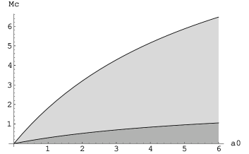
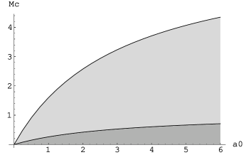
Figure 3: Forbidden regions from LEP data (dark) and expected reach of NLC (shaded) in the case of BKT at one brane $a_{\pi}=0$ (left) and BKT equal at both branes $a_{\pi}=a_{0}$ (right).

It is worth noting that although the masses (wave functions) of the heavy KK fermions get more (less) reduced for BKT at just one brane than for BKT at both branes, as shown in figures 1 and 2, the excluded regions by LEP and NLC in figure 3 are larger in the former case. This is so because what determines the $V$ limits are the gauge boson wave functions, which alternate sign with $n$ at $y=\pi R$. As can be read from the figure, in the case of UED $\!{}^{{\bf?}}$ (for which $a_{0}=a_{\pi}$) the bound coming from four-fermion contact interactions becomes more stringent for large BKT than the usually quoted one, $M_{c}>300$ GeV, coming from the $\rho$ parameter. The corrections to $\rho$ due to the extra fermion mixing induced by BKT, to be discussed below, do not improve the bounds in figure 3.

4 Yukawa Couplings

For simplicity we will only consider boundary Yukawa couplings, which are usually preferred to avoid consistency problems in supersymmetric models or more severe flavour changing neutral current restrictions. Then, the effective Yukawa couplings for the KK towers of fermions with given quantum numbers read (see, for example, Ref. $\!{}^{{\bf?}}$)

$$\lambda^{(nm)}_{ij}=\frac{\lambda^{(5)}_{ij}}{2\pi R}f^{L}_{n}(0)f^{R}_{m}(0),$$ (11)

with $i,j$ labelling the families. After electroweak symmetry breaking one obtains the standard mass matrices for quarks and leptons

$$M_{ij}=\lambda^{(00)}_{ij}\frac{v}{\sqrt{2}}.$$ (12)

These mass matrices, however, are $3\times 3$ submatrices of the infinite mass matrix involving also the KK tower of vector-like fermions. Its diagonalisation gives corrections to the masses of the observed quarks and leptons and to the CKM matrix, which is now nonunitary. The deviation from unitarity is produced by the mixing with the heavy vector-like fermions $\!{}^{{\bf?}}$. This deviation can be shown to be proportional to the mass of the light fermion (and to the inverse of the heavy one) $\!{}^{{\bf?}}$. A consequence of such scaling is that this departure from the SM is likely to be seen only for the top quark, whose charged gauge coupling to the bottom quark gets corrected:

$$W^{L}_{tb}\approx 1-\frac{1}{2}m_{t}^{2}\sum_{n>0}\Big{(}\frac{f^{t_{R}}_{n}(0)}{f^{t_{R}}_{0}(0)m_{n}}\Big{)}^{2}.$$ (13)

The effects of new vector-like fermions decouple with their masses, and hence with $M_{c}$ according to Eq. 4. The most stringent limit from precision electroweak data results from the $T$ parameter $\!{}^{{\bf?}}$. For instance, in the absence of BKT Eqs. 2 - 4 imply

$$\frac{1}{R}>2.5\mbox{ TeV, for }W^{L}_{tb}=0.992.$$ (14)

In the presence of BKT the masses and wave functions change, and so does this bound. Let us discuss the case of BKT and Yukawa couplings at one and the same brane. In figure 4 we draw the lines of constant $M_{c}$ and varying $a_{0}$ in the $W^{L}_{tb}-m_{1}$ plane, where $m_{1}$ is the mass of the lightest vector-like quark of charge $\frac{2}{3}$. $a_{0}$ grows along the lines from right to left, the initial (end) point corresponding to $a_{0}=0\ (20R)$. The shaded region is forbidden by $T$. This means that models excluded without BKT can be recovered in their presence (moving along the lines to the left). This the case of the CSM $\!{}^{{\bf?}}$, a supersymmetric five-dimensional model compactified on the orbifold $S^{1}/(Z_{2}\times Z_{2}^{\prime})$ with inverse radius $1/R\approx 350$ GeV. The $\mathcal{N}=2$ supersymmetry in the bulk forbids Yukawa couplings, which have to be included at the boundaries, where the orbifold action breaks supersymmetry down to $\mathcal{N}=1$. This model has many interesting theoretical and phenomenological features, but the mixing of the top quark with its KK excitations (with masses $m_{n}=2nM_{c}$ in this case, due to the extra orbifolding) generates too large a $T$ parameter. This is apparent in figure 4: remembering that $M_{c}$ in the figure is twice the compactification scale in this model, we see that the right end of the line $M_{c}=700$ GeV, corresponding to $1/R=350$ GeV and no BKT, is excluded. However, moving to the left along the line, this model approaches the safe region, and for large enough BKT it is reconciled with experiment  .

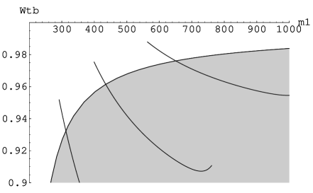
Figure 4: Value of the charged current top coupling as a function of the mass of the first KK mode in the case of BKT and Yukawa couplinga at one and the same brane. The shaded region is forbidden by the measurement of the $T$ parameter. The different lines correspond, from left to right, to $M_{c}=500,\;700,\;1000$ GeV, and the BKT $a_{0}$ increases in each line from right to left from 0 to $20R$.

5 Conclusions

Models with extra dimensions typically have lower-dimensional defects on which kinetic terms for the bulk fields can be localized. These BKT get renormalised and therefore cannot be set to zero at all scales. Moreover, it is natural that they be present already at tree level. The BKT modify the wave functions and masses of the KK modes of bulk fields, and thus their effective four-dimensional couplings. We have discussed here the effects of BKT for bulk fermions, for which relevant new effects appear both in gauge and Yukawa couplings. The former are especially relevant in the case of UED $\!{}^{{\bf?}}$, for which the bound on the compactification scale coming from four-fermion contact interactions becomes the strictest one for BKT larger than order $R$. The latter can be crucial to reconcile low scale models with boundary Yukawa couplings, like the CSM $\!{}^{{\bf?}}$, with precision electroweak measurements. Signatures of this scenario would be the observation of a reduced $W^{L}_{tb}$ mixing and the observation of a relatively light quark singlet of charge $\frac{2}{3}$, as indicates figure 4. These signals are also compatible with five-dimensional models with multilocalized fermions $\!{}^{{\bf?}}$. We want to stress again, however, that these effects require large ($\sim R$) BKT, which is not the case for BKT generated radiatively. But even small BKT can have observable phenomenological implications if they alter tree level equalities, as, for example, if they modify the mass degeneracies forbidding some decays $\!{}^{{\bf?}}$.

References

References

- [1] G. R. Dvali, G. Gabadadze and M. Porrati, Phys. Lett. B 485, 208 (2000).
- [2] H. Georgi, A. K. Grant and G. Hailu, Phys. Lett. B 506, 207 (2001).
- [3] G. R. Dvali, G. Gabadadze and M. A. Shifman, Phys. Lett. B 497, 271 (2001).
- [4] H. C. Cheng, K. T. Matchev and M. Schmaltz, Phys. Rev. D 66, 036005 (2002).
- [5] M. Carena, T. M. Tait and C. E. Wagner, Acta Phys. Polon. B 33, 2355 (2002).
- [6] B. Kyae, arXiv:hep-th/0207272.
- [7] F. del Aguila and J. Santiago, Nucl. Phys. B (Proc. Suppl.) 116, 326 (2003).
- [8] H. Davoudiasl, J. L. Hewett and T. G. Rizzo, arXiv:hep-ph/0212279.
- [9] F. del Aguila, M. Perez-Victoria and J. Santiago, JHEP 0302, 051 (2003).
- [10] M. Carena, E. Ponton, T. M. Tait and C. E. Wagner, arXiv:hep-ph/0212307.
- [11] T. Appelquist, H. C. Cheng and B. A. Dobrescu, Phys. Rev. D 64, 035002 (2001).
- [12] R. Barbieri, L. J. Hall and Y. Nomura, Phys. Rev. D 63, 105007 (2001).
- [13] T. G. Rizzo and J. D. Wells, Phys. Rev. D 61, 016007 (2000).
- [14] F. del Aguila and J. Santiago, JHEP 0203, 010 (2002).
- [15] F. del Aguila, M. Perez-Victoria and J. Santiago, JHEP 0009, 011 (2000).
- [16] F. del Aguila and J. Santiago, Phys. Lett. B 493, 175 (2000); F. del Aguila and J. Santiago, arXiv:hep-ph/0011143.
- [17] J. A. Aguilar-Saavedra, Phys. Rev. D 67, 035003 (2003).