QCD Condensates for the Light Quark V-A Correlator

Abstract

We use the procedure of pinched-weight Finite Energy Sum Rules (pFESR) to determine the OPE coefficients $a_{6},\cdots,a_{16}$ of the flavor $ud$ V-A correlator in terms of existing hadronic $\tau$ decay data. We show by appropriate weight choices that the error on the dominant $d=6$ contribution, which is known to be related to the $K\rightarrow\pi\pi$ matrix elements of the electroweak penguin operator in the chiral limit, may be reduced to below the $\sim 15\%$ level. The values we obtain for OPE coefficients with $d>8$ are shown to naturally account for the discrepancies between our results for the $d=6$ and $d=8$ terms and those of previous analyses, which were obtained neglecting $d>8$ contributions.

I Introduction

In a recent work [1], a pFESR analysis of the flavor $ud$ two-point V-A current correlator, $\Delta\Pi(Q^{2})$, was performed. This allowed extraction of the dimension six V-A OPE coefficient, $a_{6}$, which is related by chiral symmetry to the $K\rightarrow\pi\pi$ matrix element of the electroweak penguin operator, $Q_{8}$. The result for $a_{6}$ led directly to an improved determination of $\epsilon^{\prime}/\epsilon$ in the chiral limit.

The current paper is devoted to a more detailed account of this analysis. In it, we present the rationale for our choice of weight functions, describe the calculation of higher dimension OPE contributions, and discuss the relation of our work to previous treatments of the V-A correlator. Advantages of the particular version of the FESR formulation employed in our analysis are pointed out.

A Background

We recall that non-strange hadronic $\tau$ decay data provide access to the spectral functions of the flavor $ud$ vector (V) and axial vector (A) current correlators [2, 3, 4, 5]. With $J^{\mu}_{V,A}$ the standard V, A currents and the standard definitions of the spin $J=0,1$ parts of the correlators,

$$i\int d^{4}x\,e^{iq\cdot x}\langle 0|T\Bigl{(}J^{\mu}_{V,A}(x)J^{\nu}_{V,A}(0)^{\dagger}\Bigr{)}|0\rangle\equiv\left(-g^{\mu\nu}q^{2}+q^{\mu}q^{\nu}\right)\,\Pi_{V,A}^{(1)}(q^{2})+q^{\mu}q^{\nu}\,\Pi_{V,A}^{(0)}(q^{2})\,,$$ (1)

the ratios

$$R_{V,A}\equiv\frac{\Gamma[\tau^{-}\rightarrow\nu_{\tau}\,{\rm hadrons_{V,A}}\,(\gamma)]}{\Gamma[\tau^{-}\rightarrow\nu_{\tau}e^{-}{\bar{\nu}}_{e}(\gamma)]},$$ (2)

(with $(\gamma)$ indicating additional photons or lepton pairs) are expressible as weighted integrals over the corresponding spectral functions $\rho^{(J)}_{V,A}\equiv{\frac{1}{\pi}}\,{\rm Im}\,\Pi^{(J)}_{V,A}$. Working with the combinations $\Pi_{V,A}^{(0+1)}(s)\equiv\Pi_{V,A}^{(0)}(s)+\Pi_{V,A}^{(1)}(s)$ and $s\Pi_{V,A}^{(0)}(s)$, which have no kinematic singularities, one has explicitly [2, 3, 4, 5],

$$R_{V,A}=12\pi^{2}S_{EW}\,|V_{ud}|^{2}\int^{m_{\tau}^{2}}_{0}{\frac{ds}{m_{\tau}^{2}}}\,\left(1-{\frac{s}{m_{\tau}^{2}}}\right)^{2}\left[\left(1+2{\frac{s}{m_{\tau}^{2}}}\right)\,\rho^{(0+1)}_{V,A}(s)-\,{\frac{2s}{m_{\tau}^{2}}}\,\rho^{(0)}_{V,A}(s)\right]\,$$ (3)

where $S_{EW}=1.0194\pm 0.0040$ represents the leading electroweak corrections [6], and $V_{ud}$ is the $ud$ CKM matrix element . Since the integrals over the $J=0$ part of the spectral function are saturated by the pion pole contribution, up to numerically negligible corrections of ${\cal O}(m_{u,d}^{2})$, non-strange hadronic $\tau$ decay data provide detailed information on the sum $\rho_{V}^{(0+1)}(s)+\rho_{A}^{(0+1)}(s)$. For states containing only pions, G-parity allows an unambiguous separation of the V and A components of this sum. In the range where the decay to states containing kaon pairs is negligible (say $s\leq 2~{}{\rm GeV}^{2}$), the individual V and A terms, and hence also the difference $\Delta\rho\equiv\rho_{V}^{(0+1)}$-$\rho_{A}^{(0+1)}$, are thus known very accurately from experiment.

Knowledge of the V and A spectral functions allows access to the corresponding correlators through the use of either dispersion relations or FESR’s. The latter may be taken to have the form

$$\int_{s_{th}}^{s_{0}}\,ds\,\rho(s)\,w(s)\,={\frac{-1}{2\pi i}}\,\oint_{|s|=s_{0}}\,ds\,\Pi(s)w(s)\ ,$$ (4)

valid for any $w(s)$ analytic in the region of the contour, and any $\Pi(s)$ without kinematic singularities. An example is the standard OPE representation of $R_{V,A}$ [2, 3, 4, 5],

$$R_{V,A}=6\pi S_{EW}\,|V_{ud}|^{2}i\,\oint_{|s|=m_{\tau}^{2}}{\frac{ds}{m_{\tau}^{2}}}\,\left(1-{\frac{s}{m_{\tau}^{2}}}\right)^{2}\left[\left(1+2{\frac{s}{m_{\tau}^{2}}}\right)\Pi^{(0+1)}_{V,A}(s)-2{\frac{s}{m_{\tau}^{2}}}\,\Pi^{(0)}_{V,A}(s)\right]\,,$$ (5)

which results from the application of Eq. (4) to Eq. (3).

If one works at sufficiently large $s_{0}$ that the OPE representation of $\Pi(s)$ may be used reliably on the RHS of Eq. (4), appropriate choices for the weight $w(s)$ allow one to determine OPE contributions of different dimension, $d$, in terms of experimental data for $\rho(s)$ (analogous statements are true for the corresponding dispersion relations and/or their Borel transforms). To reflect the fact that $\Pi(s)$ will differ from its OPE representation over at least some portion of the contour $|s|=s_{0}$, we recast Eq. (4) in the general form

$$\int_{s_{th}}^{s_{0}}\,ds\,\rho(s)\,w(s)\,+R[s_{0},w]={\frac{-1}{2\pi i}}\,\oint_{|s|=s_{0}}\,ds\,\Pi_{\rm OPE}(s)\,w(s)\ ,$$ (6)

where

$$R[s_{0},w]\equiv{\frac{-1}{2\pi i}}\,\oint_{|s|=s_{0}}\,ds\,\left(\Pi_{\rm OPE}(s)-\Pi(s)\right)\,w(s)\ \ .$$ (7)

$R[s_{0},w]$ then quantifies what is usually referred to as “OPE breakdown” or “duality violation”.

Due to the intractibility of strong-coupling QCD, it is not possible at present to obtain an analytic expression for $R[s_{0},w]$, and its neglect (common to all FESR analyses) therefore represents a key dynamical assumption. There exist several strategies, however, to minimize the impact of this assumption:

• Work at the highest possible $s_{0}\equiv s_{max}$, where $s_{max}$ is the maximum value of $s$ for which $\rho(s)$ is experimentally known. At high $s_{0}$, one has increased confidence in the reliability of the OPE. One can check the stability of any nominal OPE output against changes in $s_{0}$ to assess theoretical uncertainties associated with possible OPE breakdown.

• Work in the vicinity of certain ‘optimal’ $s_{0}$ values $s_{0}^{(d)}$, called duality points [9]. The set of all such $s_{0}^{(d)}$ is nothing but the zeros of $R[s_{0},w]$ for certain special weight choices. By “special” is meant that the zeros can be determined independent of the values of any unknown OPE condensates. For example, the weights $w(s)=1$ and $w(s)=s$ are special for the V-A correlator, since the $d=2$ and $d=4$ OPE contributions are known to be zero in the chiral limit (this is the OPE statement of the two Weinberg sum rules (WSR’s) [10]). In general, the sets of zeros of $R[s_{0},w]$ for different correlators and/or different weights are different. The duality point approach relies on the observation that, for the V-A correlator, the $w(s)=1$ duality points lie close to the corresponding $w(s)=s$ duality points (two such points exist in the interval $0<s_{0}<m_{\tau}^{2}$). This is taken to suggest the possibility that the zeros of $R[s_{0},w]$ for all $w(s)$ might be (approximately) the same. If so, sum rules based on other weights would be reasonably satisfied at the $w(s)=1$, $w(s)=s$ duality points. Such sum rules, restricted to these values of $s_{0}$, could then be used to extract unknown OPE coefficients. However, the uncertainty about how close the true duality point for a given sum rule is to that for the $w(s)=1,s$ sum rules will produce a corresponding uncertainty in the extracted OPE coefficients. This uncertainty can be large if the $s_{0}$ dependence of the corresponding spectral integrals is strong (as it is, for example, for the weights $w(s)=s^{k}$ with $k\geq 2$).

• Work with ‘pinched weights’, i.e., those satisfying $w(s_{0})=0$. Such weights suppress OPE contributions from the region of the contour near the timelike real axis where $\left[\Pi_{OPE}-\Pi\right]$ is expected to be largest [12]. $R[s_{0},w]$ will then be small at those scales, $s_{0}$, for which the region of OPE breakdown, on the contour $|s|=s_{0}$, is restricted to the vicinity of the timelike point. If the region of scales for which this is true extends down as far as the experimentally accessible region, one can find a window of $s_{0}$ values within which the data-based spectral integrals admit an OPE-like representation (as given by the RHS of Eq. (6)) for suitable choices of the unknown QCD parameters (i.e. the appropriate OPE condensates). A successful OPE/data match implies that $R[s_{0},w]$ is not detectable, within experimental errors, in the given analysis window. The analysis window then represents an extended duality interval, since every point in it, in the sense of the terminology above, is a duality point. Moreover, working with weights which differ significantly in the ways they weight the experimental spectral data, but whose integrated OPE contributions involve the same set of QCD parameters, allows one to perform additional checks.

We shall follow the last of these approaches and employ pFESR’s to analyze the $ud$ V-A correlator. Evidence in support of this choice can be inferred from the results of FESR studies of the flavor $ud$ V and A correlators, where one knows with good accuracy both the data and the OPE integrals for $s_{0}$ above $\sim 2\ {\rm GeV}^{2}$. These studies show that FESR’s based on the unpinched weights, $w(s)=s^{k}$ ($k=0,\cdots,3$), are rather poorly satisfied over the range $2\ {\rm GeV}^{2}<s_{0}<m_{\tau}^{2}$[11, 16] (i.e., at these scales, $R[s_{0},s^{k}]$ is typically large). In contrast, the FESR predictions, Eq. (5), for $R_{V}$ and $R_{A}$, which are obtained by taking the appropriate linear combinations of the $w(s)=1,s^{2}$ and $s^{3}$ FESR’s, with $s_{0}$ set equal to $m_{\tau}^{2}$ and $R[m_{\tau}^{2},w]$ to zero, are in extremely good agreement with experiment [18, 19]. The failure of the $s^{k}$-weighted FESR’s is a manifestation of the breakdown of the OPE representation near the timelike real $s$ axis for insufficiently large $s_{0}$, as shown by Poggio, Quinn and Weinberg (PQW) [12]. The success of the OPE predictions for $R_{V,A}$ presumably arises from the suppression of this danger region by the (double) zeros of the kinematic weights at $s=m_{\tau}^{2}$ (the edge of hadronic phase space). It turns out that for any weight of the form either $w_{N}(y)=(1-y)(1+Ay)$ or $w_{D}(y)=(1-y)^{2}(1+Ay)$ (with $A$ arbitrary and $y=s/s_{0}$), the corresponding $R_{V,A}$-like pFESR is extremely well satisfied for all $s_{0}$ in the range $2\ {\rm GeV}^{2}<s_{0}<m_{\tau}^{2}$ [11, 16]. This indicates that for the separate V and A correlators, and for such “intermediate” scales, the OPE breakdown is closely localized to the vicinity of the timelike real axis. At these scales, it appears safe to neglect $R[s_{0},w]$ also for other correlators provided $w(y)$ satisfies $w(y=1)=0$, but not otherwise. A more detailed discussion of these issues may be found in Section V.

B Summary of Content

In this paper we focus on the difference $\Delta\Pi$=$\Pi_{V}^{(0+1)}-\Pi_{A}^{(0+1)}$ of the $J=0+1$ components of the flavor $ud$ V and A correlators. In the chiral limit, its OPE is purely non-perturbative, with contributions beginning at dimension $d=6$. The smallness of $m_{u,d}$ means that the physical OPE will be dominated by $d=6$ (and higher) terms, at least until one gets to extremely large scales. Accurate data for the associated spectral function $\Delta\rho$ thus allow the extraction of various vacuum condensate combinations. Of particular interest are the two condensates appearing in the $d=6$ part of $\left[\Delta\Pi\right]_{\rm OPE}$, which turn out to determine the chiral limit values of the $K\rightarrow\pi\pi$ matrix elements of the electroweak penguin operators $Q_{7,8}$ [13]. The $d>6$ terms in $\left[\Delta\Pi\right]_{\rm OPE}$, which enter dispersive sum rules for these matrix elements [14, 15], are also of phenomenological interest since a determination of their values would allow the dispersive determination of Ref. [15] to be performed at lower scales, where uncertainties associated with the classical chiral sum constraints are drastically reduced.

We will extract the higher dimension ($d>4$) terms appearing in the OPE of $\Delta\Pi$ by constructing a set of pFESR’s designed in such a way as to minimize the impact of experimental errors. As we will show below, it is possible to make such determinations for $d=6,\cdots,16$ with good accuracy using the existing experimental $\tau$ decay data base.

In Section II, we detail the input required for the OPE and data sides of the flavor $ud$ V-A $\tau$ decay sum rules and discuss some practical considerations relevant to the choice of pFESR weight. In Section III, we describe how, by appropriate pFESR choices, it is possible to (1) significantly improve on previous determinations of the $d=6$ and $d=8$ OPE contributions and (2) at the same time, extract OPE contributions with dimensions $d=10,\cdots,16$ not obtained in those earlier analyses. A comparison with previous analyses is presented in Section IV. An expanded discussion of the issue of duality violation is given in Section V. This section also contains an outline of the techniques we have employed to test for the presence of possible residual duality violation in our analysis of the V-A correlator. Certain details of these tests which are relevant to the comparison to earlier work are deferred to the Appendix. Our conclusions, together with a brief discussion, are given in Section VI. The implications of our results for the chiral-limit values of the electroweak penguin matrix elements have already been worked out in Ref. [1].

II Sum Rule Analyses of the V-A Correlator $\Delta\Pi$

We now describe the input required for the OPE and data sides of the flavor $ud$ V-A sum rules. The emphasis is on practical considerations relevant to the choice of pFESR weight functions.

A The data side

We shall employ both the ALEPH and OPAL data for $\Delta\rho$ [18, 19]. The respective ALEPH and OPAL spectral functions are displayed in Fig. 1 .

In the case of ALEPH, we use the publicly available data files corresponding to the 1998 analysis, whose overall normalization was set by the preliminary result for the rescaled total strange hadronic branching fraction, $R_{us}\equiv B_{us}/B_{e}$, $R_{us}=0.155$, and the 1998 PDG values of $B_{e}$ and $B_{\mu}$. The 1999 published version, $R_{us}=0.161$ [20] and the recent update, $R_{us}=0.1625$ [21, 22] both differ slightly from the preliminary value. This change, together with minor changes in the values of $B_{e}$, $B_{\mu}$ and the $\tau\rightarrow\pi\nu_{\tau}$ branching fraction, $B_{\pi}$, necessitates a small global rescaling of the 1998 V-A data and covariance matrix . An input value of $V_{ud}$ is required to convert from the experimental number distribution provided by ALEPH to $\Delta\rho$. We have taken this to be $V_{ud}=0.9742\pm 0.0016$, a value which spans both the range based on the $K_{e3}$ decay analysis and that based on the combination of $0^{+}\rightarrow 0^{+}$ nuclear decays and neutron decay, as quoted in PDG2002 [23]. In the case of OPAL, we use the publicly available data files for $\Delta\rho$ and its correlation matrix, corresponding to the results of Ref. [19]. These files were constructed using a central value $V_{ud}=0.9753$. We have, therefore, performed a small global rescaling in order to work with ALEPH and OPAL versions of the spectral function which both correspond to $V_{ud}=0.9742\pm 0.0016$.

As noted previously, the data are very accurate below $s\sim 2\ {\rm GeV}^{2}$. Near the kinematic endpoint $y_{\tau}=1$ ($y_{\tau}\equiv s/m_{\tau}^{2}$), however, the errors on $\Delta\rho$ become large. This is a consequence of several factors:

1. The event rate becomes small in that region due to phase space suppression.

2. There is, at present, no complete separation of V and A contributions to the spectrum for states containing a $K\bar{K}$ pair and $\geq 1$ $\pi$’s.

3. In order to extract $\Delta\rho$ from the experimental decay distribution (c.f. Eq. (3)) one must divide by the kinematic weight factor $w_{\tau}(y_{\tau})=(1-y_{\tau})^{2}(1+2y_{\tau})$. The double zero of $w_{\tau}$ at $s=m_{\tau}^{2}$ thus amplifies the errors on the V-A number distributions for those $s$ near $s=m_{\tau}^{2}$.

In view of item $3$, pinched weights with only a single zero at $s=s_{0}$ will weight the experimental number distribution and errors with a factor which diverges as $s\rightarrow s_{0}$ for $s_{0}$ near $m_{\tau}^{2}$. Such behavior is to be avoided if one wishes to keep the errors on the weighted spectral integrals under control. For this reason we restrict our attention in the following to pFESR’s based on polynomial weights of the form $p(y)(1-y)^{2}$ ($y\equiv s/s_{0}$). Though this restriction is forced on us by necessity, it has the virtue of enforcing a stronger suppression of OPE contributions from the vicinity of the timelike real axis, and hence of improving the reliability of the OPE side of the pFESR’s.

An important practical consideration in choosing pFESR weights is the non-positive definiteness of $\Delta\rho$. Even with the very precise data below $2\ {\rm GeV}^{2}$, weighted integrals which involve significant cancellations between contributions from the regions of positive and negative $\Delta\rho$ will have much larger fractional errors than would be expected based only on the accuracy of the spectral data alone. For some of the weights employed previously in the literature, for example, the V-A cancellation is at the level of a few percent of the individual V and A integrals, leading to large errors and significant sensitivities (as large as $20\%$) to the exact treatment of the $\pi$ pole contribution. Avoiding strong cancellations of this type is crucial to reducing the errors on the final determinations of the various vacuum condensates. To quantify this point in our discussions below, we introduce a quantity $r_{V-A}$ defined as the ratio of the V-A spectral integral to the corresponding vector spectral integral.

B The OPE side

The OPE representation of $\Delta\Pi$ is schematically of the form

$$\Delta\Pi(Q^{2})=\sum_{d=2,4,\cdots}{\frac{X_{d}}{Q^{d}}}\ ,$$ (8)

where $Q^{2}=-s$. Perturbative corrections lead to logarithmic dependences of the $X_{d}$ on $Q^{2}$. To NLO in QCD one has:

$$X_{d}=a_{d}(\mu)+b_{d}\,\log\left(\frac{Q^{2}}{\mu^{2}}\right)\ .$$ (9)

The $b_{d}(\mu)$ are known explicitly for $d=2,4,6$, but not for higher $d$. For polynomial weights, OPE contributions proportional to $b_{d}(\mu)$ involve the integrals $\int_{|x|=1}\,dx\ x^{k}\,log(x)$. For the weights $w(y)=p(y)(1-y)^{2}$ employed in our analysis the variations of sign in the coefficients of $w(y)$ produce significant cancellations (and hence additional numerical suppressions) of these contributions relative to those of the leading non-logarithmic terms. We thus consider it very safe to follow earlier analyses in neglecting such corrections for $d\geq 8$. The remaining non-logarithmic OPE integral contributions follow from

$${\frac{-1}{2\pi i}}\,\oint_{|s|=s_{0}}\,ds\,\left[{\frac{a_{d}}{Q^{d}}}\right]\left({\frac{s}{s_{0}}}\right)^{k}=(-1)^{k}\,\delta_{k,(d/2)-1}\,\left[{\frac{a_{d}}{s_{0}^{k}}}\right]\ .$$ (10)

Weights of degree $2$ thus contain leading OPE contributions up to $d=6$, those of degree $3$ contributions up to $d=8$, etc.. Neglect of $d=10,\cdots,2N+2$ contributions in pFESR’s based on weights with degree $N>3$ is therefore dangerous unless one is working at $s_{0}$ large enough that such contributions may be taken to be safely small. Typically one does not know a priori how large an $s_{0}$ is “large enough”; however, the stronger $1/s_{0}$-dependence of the higher $d$ integrals allows this question to be addressed post facto, provided one works with a range of $s_{0}$ large enough to expose the presence of higher $d$ contributions which may have been omitted when they should not have been. If one finds that the range of $s_{0}$ employed is such that the presence of such contributions is indicated, one can use the pFESR in question to place constraints on the relevant higher dimension $a_{d}$ terms. Obviously, both the reliability of the post facto check and the accuracy of the higher $d$ extraction will be enhanced for pFESR’s having fewer separate $a_{d}$ contributions on the OPE side of the sum rule and larger separations between the dimensions of the contributions which do occur.

The $d=2$ term in Eq. (8) is of ${\cal O}(m_{u,d}^{2})$. That it can be safely neglected can be confirmed numerically by integrating the $J=0+1$ expression of Ref. [25], which is known to ${\cal O}(\alpha_{s}^{2})$. 

The $d=4$ term in Eq. (8) is given by [3, 29]

$$\left[\Delta\Pi(Q^{2})\right]_{d=4}=\left({\frac{8}{3}}\bar{a}+{\frac{59}{3}}\bar{a}^{2}\right){\frac{\langle(m_{u}+m_{d})\bar{u}u\rangle}{Q^{4}}}\ ,$$ (11)

where $\bar{a}\equiv\alpha_{s}(Q^{2})/\pi$, with $\alpha_{s}(Q^{2})$ the running coupling at scale $\mu^{2}=Q^{2}$ in the $\overline{MS}$ scheme. The quark condensate factor can be evaluated using the GMOR relation [30]

$$\langle(m_{u}+m_{d})\bar{u}u\rangle=-F_{\pi}^{2}m_{\pi}^{2}\ ,$$ (12)

which is accurate to better than $6\%$ [31]. We compute the weighted integrals of $\left[\Delta\Pi(Q^{2})\right]_{d=4}$ using the “contour improvement” scheme [4, 32], taking for $\bar{a}$ the version corresponding to 4-loop running [33] with the ALEPH determination [18] $\alpha_{s}(m_{\tau}^{2})=0.334\pm 0.022$ as input. This contribution represents only a small correction to the dominant $d=6$ term because of the ${\cal O}(m_{u,d})$ chiral suppression. In the numerical analysis we have expanded to $\pm 20\%$ the errors assigned to the GMOR evaluation of the $d=4$ OPE contributions in order to account for the truncation of the series for the Wilson coefficient at ${\cal O}(\bar{a}^{2})$. Because the $d=4$ contribution is so small, the resulting contribution to the total error is, however, negligible.

Observe that in the chiral limit the $d=2$ and $d=4$ contributions are zero. Taking $a_{2}=a_{4}=0$ is then the OPE implementation of the first and second WSR’s. To the extent that we use $a_{2}=0$ and $a_{4}\sim m_{\pi}^{2}$ the WSR’s are built into our procedure.

For the $d=6$ contribution, there exist several determinations in the literature [15, 34, 35], corresponding to different schemes for the choice of evanescent operator basis [36]. Since one of our goals is to use our results for the $d=6$ contribution to improve the determination of the chiral limit value of the electroweak penguin contribution to the $K\rightarrow\pi\pi$ decay amplitudes, we employ the most recent determination [15], which corresponds to the same scheme as used in the calculation of the Wilson coefficients of the effective weak Hamiltonian [37] . To simplify the later application of our results it is also convenient to work with the vacuum condensates $\langle O_{1}\rangle$ and $\langle O_{8}\rangle$ defined in Ref. [15],

$$\langle O_{1}\rangle = \langle{\bar{q}}\gamma_{\mu}{\frac{\tau_{3}}{2}}q~{}{\bar{q}}\gamma^{\mu}{\frac{\tau_{3}}{2}}q-{\bar{q}}\gamma_{\mu}\gamma_{5}{\frac{\tau_{3}}{2}}q~{}{\bar{q}}\gamma^{\mu}\gamma_{5}{\frac{\tau_{3}}{2}}q\rangle\ ,$$ (13)

$$\langle O_{8}\rangle = \langle{\bar{q}}\gamma_{\mu}\lambda^{a}{\frac{\tau_{3}}{2}}q~{}{\bar{q}}\gamma^{\mu}\lambda^{a}{\frac{\tau_{3}}{2}}q-{\bar{q}}\gamma_{\mu}\gamma_{5}\lambda^{a}{\frac{\tau_{3}}{2}}q~{}{\bar{q}}\gamma^{\mu}\gamma_{5}\lambda^{a}{\frac{\tau_{3}}{2}}q\rangle\ ,$$ (14)

where $q=u,d,s$, $\tau_{3}$ is a Pauli (flavor) matrix, and $\{\lambda^{a}\}$ are the Gell Mann color matrices. With these choices one has

$$\left[\Delta\Pi(Q^{2})\right]_{d=6}={\frac{1}{Q^{6}}}\left[a_{6}(\mu)+b_{6}(\mu)\ln{Q^{2}\over\mu^{2}}\right]\ ,$$ (15)

with

$$a_{6}(\mu) = 2\left[2\pi\langle\alpha_{s}O_{8}\rangle_{\mu}+A_{8}\langle\alpha_{s}^{2}O_{8}\rangle_{\mu}+A_{1}\langle\alpha_{s}^{2}O_{1}\rangle_{\mu}\right]\ ,$$ (16)

$$b_{6}(\mu) = 2\left[B_{8}\langle\alpha_{s}^{2}O_{8}\rangle_{\mu}+B_{1}\langle\alpha_{s}^{2}O_{1}\rangle_{\mu}\right]\ ,$$ (17)

where $A_{1}$, $A_{8}$, $B_{1}$ and $B_{8}$ are the coefficients tabulated in Ref. [15] . They depend on the number of active flavors, the scheme employed for $\gamma_{5}$, and the evanescent operator basis. For $N_{f}=3$, the values for the NDR and HV $\gamma_{5}$ schemes are

$$A_{1} = 2\ ({\rm NDR}),\ -10/3\ ({\rm HV})$$ (18)

$$A_{8} = 25/4\ ({\rm NDR}),\ 21/4\ ({\rm HV})$$ (19)

$$B_{1} = 8/3\ ({\rm NDR\ and\ HV})$$ (20)

$$B_{8} = -1\ ({\rm NDR\ and\ HV})\ .$$ (21)

The logarithmic ($B_{1,8}$) terms turn out to play a very small role in the analysis, though we have kept them for completeness. We do this by first writing $b_{6}=a_{6}(b_{6}/a_{6})$ and then employing the existing dispersive determination of $\langle O_{1}\rangle$ and $\langle O_{8}\rangle$ [15] to estimate $r_{6}=b_{6}/a_{6}$. With this estimate as input, the integrated $d=6$ OPE contribution is now, like the non-logarithmic $d=6$ term, proportional to $a_{6}$. The overall $a_{6}$ factor multiplying the full $d=6$ contribution is then to be fit to data. The central value for $r_{6}$ turns out to be very small, $\simeq-0.03$. Since only the first term in the expansion of $b_{6}$ in powers of $\alpha_{s}$ is known, we assign a (conservative) $50\%$ uncertainty to this estimate.

For $d=8$ and higher we take

$$\left[\Delta\Pi(Q^{2})\right]_{d}={\frac{a_{d}}{Q^{d}}}\ .$$ (22)

With this notation, $a_{8}$ is identical to $\langle O_{8}\rangle$ of Ref. [8] and $O_{8}$ of Ref. [24]. It is also twice the negative of the integral $M_{3}$ of Ref. [38, 39], independent of $s_{0}$, in the absence of duality violation in the $s^{3}$-weighted FESR.

III Extraction of OPE Condensates from pFESR’s

A Choice of pFESR Weights and the $s_{0}$ Analysis Window

We consider a sequence of pFESR’s designed to simplify the extraction of the OPE coefficients $a_{d}$ of $\Delta\Pi$. Working with pFESR’s allows us to take advantage of the freedom in the choice of weight profile, and hence, by construction, to avoid strong V-A cancellations. The freedom of weight choice also allows us to considerably simplify the task of constraining the $d>8$ contributions and separating them from the $d=6$ and $d=8$ contributions.

Within the space of pFESR weights $w(y)=p(y)(1-y)^{2}$ employed in our analysis, the weight of lowest possible degree is $w(y)=(1-y)^{2}$. In a zero-error world, the corresponding pFESR would allow an extraction of $a_{6}$. Unfortunately, this weight produces a high degree of V-A cancellation, and hence is not practical for use when employed with present experimental data. We thus consider weights of degree 3 (the highest degree possible involving no $a_{d}$ contributions with $d>8$), $w(y)=(1-y)^{2}(1+Ay)$. There will be some value of $A$ for which the fractional errors on the spectral integrals are minimized. It turns out that this value is almost exactly equal to $-3$. The pFESR based on

$$w_{1}(y)=(1-y)^{2}(1-3y)$$ (23)

will then provide the most restrictive constraint on $a_{6}$, $a_{8}$, and this is our first choice of weight. The weight $w_{2}(y)=y(1-y)^{2}$ also has reduced V-A cancellation, and provides independent constraints on the determination of $a_{6}$ and $a_{8}$, since degree three polynomials yield only $a_{4}$, $a_{6}$ and $a_{8}$ OPE contributions, and $a_{4}$ is small. The $s_{0}$ dependence of both the $w_{1}$- and $w_{2}$-weighted spectral integrals will be well-described using only two parameters, $a_{6}$ and $a_{8}$, provided the use of the OPE representation is justified. $w_{2}$ has been chosen, by construction, to weight $\Delta\rho(s)=\Delta\rho(s_{0}y)$ with a profile very different from $w_{1}$ to make this test of the reliability of the OPE representation as non-trivial as possible.

We determine our $s_{0}$ analysis window by fixing the upper edge at $s_{0}=3.15\ {\rm GeV^{2}}\simeq m_{\tau}^{2}$ and decreasing the lower edge until the fitted coefficients cease to be consistent (within experimental errors). Since $a_{6}$ is the most accurately determined coefficient we use it as our basic monitor of the onset of duality violation. We find that duality violation for the V-A correlator and the $w_{1}$, $w_{2}$ weight set begins to set in below $s_{0}\sim 1.8\ {\rm GeV}^{2}$, and hence we fix the lower edge of our analysis window at $1.95\ {\rm GeV^{2}}$.

To investigate $d>8$ contributions it is convenient to construct weights for which the only OPE contributions with $d>4$ are those proportional to $a_{6}$ and $a_{d}$, with $d=10,12,\cdots$. The possibility of working with $s_{0}$ down to $\sim 2\ {\rm GeV}^{2}$ is also helpful since an increased range of $s_{0}$ creates an increased variation in the relative size of the $d=10,12,\cdots$ and $d=6$ contributions over the analysis window, and hence improves our ability to perform the separation of contributions of different dimension. Weights having a double zero at $y=1$, reduced V-A cancellation, and only a single $a_{d}$ contribution beyond $d=6$, are

$$w_{N}(y)=y\left[1-\left({\frac{N}{N-1}}\right)y+\left({\frac{1}{N-1}}\right)y^{N}\right]\ \qquad N=2,3,4,5,6\ .$$ (24)

The overall factor of $y$ has been introduced in order to reduce the level of V-A cancellation. The case $N=2$ corresponds to the previously introduced weight $w_{2}=y(1-y)^{2}$. For $N>2$, $w_{N}(y)$ produces contributions proportional to $a_{4}$, $a_{6}$ and $a_{2N+4}$ on the OPE side of the sum rule. We consider $N$ up to $6$, and hence $a_{d}$ contributions with $d$ up to $16$.  Since each of the resulting sum rules allows a determination of both $a_{6}$ and $a_{2N+4}$, the consistency of the $a_{6}$ solutions obtained from the $w_{1}$ through $w_{6}$ pFESR’s also provides a strong self-consistency constraint on the reliability of the analysis. Further constraints on $a_{8}$ and the higher dimension $a_{d}$ can be obtained by considering the weights

$$w_{4+N}(y)=y\left[1-\left({\frac{N}{N-2}}\right)y^{2}+\left({\frac{2}{N-2}}\right)y^{N}\right]\ \qquad N=3,4,5,6\ .$$ (25)

These weights produce $a_{4}$, $a_{8}$ and $a_{d}$ contributions with $d=10,12,14$ and $16$ for $N=3,4,5$ and $6$, respectively. The $a_{8}$ and $a_{d>8}$ values extracted using $w_{7}$ through $w_{10}$ should be consistent with those obtained using $w_{1}$ through $w_{6}$, provided the OPE representation of $\Delta\Pi$ is reliable for the $s_{0}$ employed in our analysis. We find the consistency is excellent for all the $a_{d}$ with $d>4$.

Finally, we observe that pFESRs based on the weights of Eqs. (24) and (25) allow one in principle to extract condensates of even higher dimension. With the present experimental errors, however, higher degree pFESR’s effectively work with a smaller analysis window, localized around $s_{0}=2$ GeV² (points at higher $s_{0}$ suffer from much larger experimental errors, and become irrelevant in the analysis). This feature weakens the power of this method to detect inconsistencies through the use of an extended $s_{0}$ analysis window. We therefore quote our results for the condensates only up to $d=16$.

With the above choice of weights, and assuming $R[s_{0},w]=0$, the $w_{1}$ through $w_{10}$ pFESR’s may be written as

$$J_{w_{n}}(s_{0})=f_{w_{n}}(\{a_{d}\};s_{0})$$ (26)

where

$$J_{w_{n}}(s_{0}) = \int_{0}^{s_{0}}ds\,w_{n}\left(\frac{s}{s_{0}}\right)\,\Delta\rho(s)+{\frac{1}{2\pi i}}\oint_{|s|=s_{0}}ds\,w_{n}\left(\frac{s}{s_{0}}\right)\,\left[\Delta\Pi_{\rm OPE}(s)\right]_{d=4}$$ (27)

$$f_{w_{n}}(\{a_{d}\};s_{0}) = -{\frac{1}{2\pi i}}\oint_{|s|=s_{0}}ds\,w_{n}\left(\frac{s}{s_{0}}\right)\,\left[\Delta\Pi_{\rm OPE}(s)\right]_{d>4}\ .$$ (28)

The explicit form for the OPE integrals is:

$$f_{w_{1}}(\{a_{d}\};s_{0}) = {\frac{7}{s_{0}^{2}}}\,a_{6}\,\left[1+r_{6}\,\log\left({\frac{s_{0}}{\mu^{2}}}\right)+{\frac{3}{14}}r_{6}\right]\,+\,{\frac{3a_{8}}{s_{0}^{3}}}$$ (29)

$$f_{w_{2}}(\{a_{d}\};s_{0}) = -{\frac{2}{s_{0}^{2}}}\,a_{6}\,\left[1+r_{6}\,\log\left({\frac{s_{0}}{\mu^{2}}}\right)\right]\,-\,{\frac{a_{8}}{s_{0}^{3}}}$$ (30)

$$f_{w_{3}}(\{a_{d}\};s_{0}) = -{\frac{3}{2s_{0}^{2}}}\,a_{6}\,\left[1+r_{6}\,\log\left({\frac{s_{0}}{\mu^{2}}}\right)+{\frac{1}{2}}r_{6}\right]\,+\,{\frac{a_{10}}{2s_{0}^{4}}}$$ (31)

$$f_{w_{4}}(\{a_{d}\};s_{0}) = -{\frac{4}{3s_{0}^{2}}}\,a_{6}\,\left[1+r_{6}\,\log\left({\frac{s_{0}}{\mu^{2}}}\right)+{\frac{2}{3}}r_{6}\right]\,-\,{\frac{a_{12}}{3s_{0}^{5}}}$$ (32)

$$f_{w_{5}}(\{a_{d}\};s_{0}) = -{\frac{5}{4s_{0}^{2}}}\,a_{6}\,\left[1+r_{6}\,\log\left({\frac{s_{0}}{\mu^{2}}}\right)+{\frac{3}{4}}r_{6}\right]\,+\,{\frac{a_{14}}{4s_{0}^{6}}}$$ (33)

$$f_{w_{6}}(\{a_{d}\};s_{0}) = -{\frac{6}{5s_{0}^{2}}}\,a_{6}\,\left[1+r_{6}\,\log\left({\frac{s_{0}}{\mu^{2}}}\right)+{\frac{4}{5}}r_{6}\right]\,-\,{\frac{a_{16}}{5s_{0}^{7}}}$$ (34)

$$f_{w_{7}}(\{a_{d}\};s_{0}) = -{\frac{3}{s_{0}^{2}}}r_{6}a_{6}\,+\,{\frac{3a_{8}}{s_{0}^{3}}}+\,{\frac{2a_{10}}{s_{0}^{4}}}$$ (35)

$$f_{w_{8}}(\{a_{d}\};s_{0}) = -{\frac{8}{3s_{0}^{2}}}r_{6}a_{6}\,+\,{\frac{2a_{8}}{s_{0}^{3}}}-\,{\frac{a_{12}}{s_{0}^{5}}}$$ (36)

$$f_{w_{9}}(\{a_{d}\};s_{0}) = -{\frac{5}{2s_{0}^{2}}}r_{6}a_{6}\,+\,{\frac{5a_{8}}{3s_{0}^{3}}}+\,{\frac{2a_{14}}{3s_{0}^{6}}}$$ (37)

$$f_{w_{10}}(\{a_{d}\};s_{0}) = -{\frac{12}{5s_{0}^{2}}}r_{6}a_{6}\,+\,{\frac{3a_{8}}{2s_{0}^{3}}}-\,{\frac{a_{16}}{2s_{0}^{7}}}\ .$$ (38)

Note that the small, known $d=4$ OPE contribution has been moved to the spectral integral side in defining $J_{w_{n}}(s_{0})$.

B pFESR Fit: Input and Results

For our final results, we proceed in two steps. In the first step, we extract a preferred value for $a_{6}$ in an analysis employing only the weights $w_{1}$ and $w_{2}$ [1]. Such an analysis is “maximally safe” in the sense that the numerical suppressions of the integrated $d>8$ OPE logarithmic corrections are strongest when $d-2n$, where $n$ is the degree of the pFESR polynomial, is as large as possible; the neglect of such $d>8$ logarithmic terms in the OPE is thus safest when one uses the weight(s) of the minimum possible degree. As explained above, the accuracy of current data means that the lowest such degree which still allows an accurate extraction of $a_{6}$ is $3$. In the second step, we perform a combined least-squares fit for the coefficients $a_{6},\cdots,a_{16}$ using, for each of the weights $w_{1}$ through $w_{10}$, defined in Eqs. (23), (24), and (25), the set of 7 $s_{0}$ values $1.95+0.2k\ {\rm GeV}^{2}$, $k=0,\cdots,6$, which span the range from $s_{0}\sim 2\ {\rm GeV}^{2}$ to $3.15\ {\rm GeV}^{2}\simeq m_{\tau}^{2}$.

On the data side we use as input for the analyses based on both the ALEPH and OPAL data $B_{e}=0.1781\pm 0.0006$ [23], $F_{\pi}=92.4\pm 0.07\pm 0.25\ {\rm MeV}$ [23], $S_{EW}=1.0194\pm 0.0040$, and $|V_{ud}|=0.9742\pm 0.0016$. The rescaling of the 1998 ALEPH data is determined using $R_{ud}\equiv B_{ud}/B_{e}=3.480\pm 0.014$ [22]. This value is based on the most recent update, $R_{us}=0.1625\pm 0.0066$ [21, 22], in combination with the PDG2002 average for $B_{e}$ (quoted above), and the assumption of $\mu$-$e$ universality. On the OPE side we use $\langle(m_{u}+m_{d})\bar{u}u\rangle=-F_{\pi}^{2}m_{\pi}^{2}$, and $r_{6}\equiv b_{6}/a_{6}=-0.030\pm 0.015$.

In listing final errors for the ALEPH-based analysis we quote separately the errors produced by the uncertainties in the ALEPH number distribution, and those due to all other sources, including the uncertainties on the OPE input quantities $a_{4}$ and $r_{6}$. The former are calculated using the rescaled ALEPH covariance matrix. The latter are combined in quadrature.

In the analysis based on the OPAL data, we again quote two uncertainties. The first is that computed using the OPAL covariance matrix, the second that obtained by combining in quadrature the errors associated with uncertainties in all other input parameters ($V_{ud}$, $S_{EW}$, $a_{4}$, and $r_{6}$).

Fits to the ALEPH data

The results of the “maximally safe” analysis for $a_{6}$ and $a_{8}$ are 

$$a_{6} = -\left(4.45\pm 0.61\pm 0.34\right)\times 10^{-3}\ {\rm GeV}^{6}$$ (39)

$$a_{8} = -\left(6.16\pm 2.78\pm 1.40\right)\times 10^{-3}\ {\rm GeV}^{8}\ .$$ (40)

For the “combined fit” analysis, we find

$$a_{6} = -\left(4.54\pm 0.83\pm 0.18\right)\times 10^{-3}\ {\rm GeV}^{6}$$ (41)

$$a_{8} = -\left(5.70\pm 3.72\pm 0.64\right)\times 10^{-3}\ {\rm GeV}^{8}$$ (42)

$$a_{10} = \ \ \left(4.82\pm 1.02\pm 0.20\right)\times 10^{-2}\ {\rm GeV}^{10}$$ (43)

$$a_{12} = -\left(1.60\pm 0.26\pm 0.05\right)\times 10^{-1}\ {\rm GeV}^{12}$$ (44)

$$a_{14} = \ \ \left(4.26\pm 0.62\pm 0.14\right)\times 10^{-1}\ {\rm GeV}^{14}$$ (45)

$$a_{16} = -\left(1.03\pm 0.14\pm 0.03\right)\ {\rm GeV}^{16}\ .$$ (46)

Fits to the OPAL data

The results of the “maximally safe” analysis for $a_{6}$ and $a_{8}$ are

$$a_{6} = -\left(5.43\pm 0.72\pm 0.25\right)\times 10^{-3}\ {\rm GeV}^{6}$$ (47)

$$a_{8} = -\left(1.35\pm 3.32\pm 1.0\right)\times 10^{-3}\ {\rm GeV}^{8}\ .$$ (48)

For the combined analysis, we find

$$a_{6} = -\left(5.06\pm 0.89\pm 0.12\right)\times 10^{-3}\ {\rm GeV}^{6}$$ (49)

$$a_{8} = -\left(3.12\pm 3.82\pm 0.45\right)\times 10^{-3}\ {\rm GeV}^{8}$$ (50)

$$a_{10} = \ \ \left(3.87\pm 1.06\pm 0.10\right)\times 10^{-2}\ {\rm GeV}^{10}$$ (51)

$$a_{12} = -\left(1.32\pm 0.27\pm 0.03\right)\times 10^{-1}\ {\rm GeV}^{12}$$ (52)

$$a_{14} = \ \ \left(3.54\pm 0.66\pm 0.06\right)\times 10^{-1}\ {\rm GeV}^{14}$$ (53)

$$a_{16} = -\left(0.85\pm 0.15\pm 0.02\right)\ {\rm GeV}^{16}\ .$$ (54)

We note that the ALEPH and OPAL determinations of OPE coefficients are in good agreement within errors. There is also extremely good agreement between the combined-fit and maximally-safe-fit values for $a_{6}$ and $a_{8}$ in both the ALEPH and OPAL cases, providing strong post facto support for the neglect of the higher $d$ logarithmic corrections. One further point of relevance to the self-consistency of the analysis, not evident from the results quoted above, is the following. For each of the ten pFESR’s considered above, it is possible, because of the different $s_{0}$-dependence of contributions of different dimension, to extract values for the two unknown ($d>4$) $a_{d}$ coefficients occuring on the OPE side of the sum rule in question. One can then compare the values of a given $a_{d}$ obtained using various different individual pFESR’s. It turns out that the agreement among the results of different single-pFESR analyses is excellent for all the $a_{d}$, $d=6,\cdots,16$. By construction six such determinations, and hence six such consistency tests, exist for $a_{6}$ and $a_{8}$.

Our combined fit leads to a determination of the six parameters $a_{6}\dots a_{16}$. Because of the strong correlations between data integrals corresponding to different $s_{0}$ and/or different weights, the resulting fit parameters are highly correlated. If $C_{DD^{\prime}}$ is the $DD^{\prime}$ element of the correlation matrix, we find that the smallest of the $|C_{DD^{\prime}}|$ is $0.90$ for the solution set associated with the ALEPH data and $0.82$ for that associated with the OPAL data. The full covariance matrices are available upon request.

C The Optimized OPE/Spectral Integral Match

It is important to verify that, after fitting the OPE coefficients $a_{d}$, the resulting OPE integrals $f_{w_{n}}(\{a_{d}\};s_{0})$ provide a good match to the corresponding spectral integrals $J_{w_{n}}(s_{0})$ over the whole of the $s_{0}$ analysis window. Failure to achieve such a match would represent a clear sign of duality violation. In Figs. 2, 3 and 4 we display the quality of the $f_{w_{n}}(\{a_{d}\};s_{0})$ / $J_{w_{n}}(s_{0})$ match for the combined fit to the ALEPH data. (The match for the combined fit to the OPAL data is of identical quality, and hence not shown separately.) Fig. 2 shows the results for the $w_{1}$ and $w_{2}$ pFESR’s, Fig. 3 for the $w_{3}$ through $w_{6}$ pFESR’s, and Fig. 4 for the $w_{7}$ through $w_{10}$ pFESR’s. Our results for $f_{w_{n}}(\{a_{d}\};s_{0})$, corresponding to Eqs. (46), are given by the solid lines. There is clearly no sign of duality violation for any of the pFESR’s employed at any of the scales, $s_{0}$, in our analysis window. Improved data would reduce the errors on $J_{w_{n}}(s_{0})$ and allow us to sharpen this test even further. Also shown for comparison in each figure are the OPE results corresponding to the $a_{6}$, $a_{8}$ fits of Refs. [8, 24], where, as in those references we take as central input values $a_{d}=0$ for $d>8$. The inclusion of $d>8$ contributions clearly leads to a significantly improved fit to the data, as well as a significantly reduced error on the determination, in particular, of $a_{6}$.

The excellent agreement between the optimized OPE representation and the corresponding data integrals displayed in Figs. 2 through 4, while a necessary condition that significant duality violation be absent from our analysis, is not a sufficient one. In order to investigate this question further, we have performed a number of additional tests on our solution sets. Since several of these tests correspond to sum rules studied in earlier analyses of the V-A correlator, we first discuss the relation between our results and those of these earlier analyses. Having introduced the relevant sum rules as part of this discussion, we will then return to a discussion of the additional tests which such sum rules allow us to perform on our solution sets in Section V.

IV Previous Analyses

Several determinations of the $d=6$ and $d=8$ contributions to the OPE of $\Delta\Pi$ exist already in the literature [8, 18, 19, 24, 38, 39, 40]. In some cases the quoted results (especially for $a_{8}$) differ significantly from ours. To pin down the source of these discrepancies, a closer scrutiny of the previous analyses is in order. In general, previous results have errors much larger than those on the spectral function over most of its measured range. This suggests either the impact of strong cancellations or the presence of additional theoretical systematic uncertainties. One obvious possibility is the presence of $d>8$ contributions, neglected in the analyses of Refs. [8, 18, 19, 24], in the solutions for $a_{6}$, $a_{8}$. We will demonstrate below that, for both $a_{6}$ and $a_{8}$, the differences between our results and those of previous analyses are naturally accounted for by the $d>8$ coefficients given in Eqs. (46), (54).

In what follows, we shall recall the basic ingredients of the earlier analyses and discuss possible sources of uncertainty.

A Spectral Weight Analyses

In Refs. [8, 18, 19], the “(k,m) spectral weights”,

$$w^{(k,m)}(y)=y^{m}(1-y)^{2+k}(1+2y)\ ,$$ (55)

with $(k,m)=(0,0)$ and $(1,m)$, $m=0,\cdots,3$, were employed to extract $a_{6}$ and $a_{8}$, under the implicit assumption that contributions with $d>8$ were negligible in all cases. The fits for $a_{6}$ and $a_{8}$ were, in all cases, performed using only the highest $s_{0}$ available, $s_{0}=m_{\tau}^{2}$.

Ref. [8] (DGHS) represents an update of the earlier ALEPH analysis [18], and concentrates specifically on the V-A combination, which was not studied independently in the original ALEPH paper. The results for $a_{6}$, $a_{8}$ thus supercede those inferred from the separate V, A extractions performed in Ref. [18]. The results, in our notation, are

$$a_{6} = \left(-6.4\pm 1.8\right)\times 10^{-3}\ {\rm GeV}^{6}$$ (56)

$$a_{8} = \left(\ \ 8.7\pm 2.4\right)\times 10^{-3}\ {\rm GeV}^{8}\ .$$ (57)

They are in good agreement with the results of the OPAL analysis [19],

$$a_{6} = \left(-6.0\pm 0.1\right)\times 10^{-3}\ {\rm GeV}^{6}$$ (58)

$$a_{8} = \left(\ \ 7.6\pm 0.6\right)\times 10^{-3}\ {\rm GeV}^{8}\ .$$ (59)

One should bear in mind that the DGHS and OPAL analysis methods are somewhat different: the DGHS results follow from a dedicated V-A analysis, while the OPAL results were generated by combining the $d=6,8$ contributions extracted for the separate V and A correlators. The separate V, A analyses, however, involve an additional OPE fitting parameter, the gluon condensate, which is absent in the V-A difference. The fits display very strong correlations between $a_{6}$, $a_{8}$ and the gluon condensate [19]. A dedicated V-A analysis of the OPAL data would thus, in general, be expected to give different results for $a_{6}$, $a_{8}$. In view of this, and the good agreement between the OPAL and DGHS results, we concentrate on the DGHS solution in the discussion which follows.

The DGHS value for $a_{6}$ is consistent with ours, within errors, but that for $a_{8}$ is not. We have studied the origin of this discrepancy, and we find that:

• The discrepancy can be understood as arising from the neglect of the $d>8$ contributions to the spectral weight sum rules employed by DGHS.

• The “(k,m) spectral weights” FESR actually provide a consistency check on our solution set.

We first note that the $(0,0)$ and $(1,0)$ pFESR’s have strong V-A cancellations, and hence large experimental errors on the data sides of the sum rules. For the $(0,0)$ case, which involves, from among the unknown $d>4$ $a_{d}$ terms, only the $a_{6}$ and $a_{8}$ contributions, $r_{V-A}\sim 3\%$ for $s_{0}=m_{\tau}^{2}$. The $(1,0)$ case, whose OPE side in principle involves $a_{6}$, $a_{8}$ and $a_{10}$, also has $r_{V-A}\sim 3\%$ for $s_{0}=m_{\tau}^{2}$. The $(1,1)$, $(1,2)$ and $(1,3)$ weights produce much less pronounced V-A cancellations , and hence must dominate the DGHS fit. Note, however, that $w^{(1,m)}(y)=y^{m}[1-y-3y^{2}+5y^{3}-2y^{4}]$; these weights thus produce numerical enhancements of the $a_{d}$, $d>8$ terms, whose presence on the OPE sides of the sum rules has been assumed to be numerically negligible (see explicit example below). The pFESR’s dominating the fit are thus those for which neglect of the $d>8$ terms is least safe.

It is easy to check that the combined fit values for $a_{10},\cdots,a_{16}$ predict non-negligible $d>8$ contributions for all the $(1,m)$ pFESR’s. Our results thus imply that the DGHS values for $a_{6}$ and $a_{8}$, which are dominated by $m=1,2,3$ cases, must contain higher dimension contamination. That the central DGHS $a_{6}$, $a_{8}$ values do not provide as good a fit to the $w_{1}$ and $w_{2}$ pFESR’s (for which $d>8$ contributions are absent) as does our combined fit is, presumably, a reflection of this contamination. Further evidence is provided by the $w_{3}$ through $w_{10}$ pFESR’s.

One can also explicitly demonstrate that the neglected $d>8$ contributions are, indeed, important for the spectral weight pFESR’s. This demonstration is most transparent for the $(1,3)$ pFESR since, in this case, the OPE integral is:

$$f_{w^{(1,3)}}(\{a_{d}\};s_{0})=-{a_{8}\over s_{0}^{3}}-{a_{10}\over s_{0}^{4}}+3\,{a_{12}\over s_{0}^{5}}+5\,{a_{14}\over s_{0}^{6}}+2\,{a_{16}\over s_{0}^{7}}\ .$$ (60)

If $d>8$ OPE contributions are indeed negligible then, rescaling $J_{w^{(1,3)}}(s_{0})$ by $s_{0}^{3}$ should produce a result, $-a_{8}$, independent of $s_{0}$.  We plot $s_{0}^{3}J_{w^{(1,3)}}(s_{0})$ for the ALEPH data in Fig. 5. The result is clearly far from constant with respect to $s_{0}$, unambiguously demonstrating the presence of non-negligible $d>8$ contributions. The solid line shows, for comparison, the predictions corresponding to the combined fit solution of Eqs. (46). The good match shows that the $d>8$ contributions produced by our solution naturally account for the discrepancy between the DGHS predictions and the experimental results.

A similar situation holds for the other spectral weight sum rules, as shown in Fig. 6. In the figure we display the $J_{w^{(k,m)}}(s_{0})$ together with the OPE expressions $f_{w^{(k,m)}}(\{a_{d}\};s_{0})$ corresponding to (i) the central values of the DGHS fit, Eqs. (57), together with $a_{d}=0$ for $d>8$, (shown by the dashed line), and (ii) our combined (ALEPH-based) fit, Eqs. (46), (shown by the solid line). In all cases, if one takes into account the errors and correlation for the DGHS fit parameters, the resulting OPE error bar overlaps the spectral integral bar at $s_{0}=m_{\tau}^{2}$, even when the central values are not in particularly good agreement. However, when one goes to lower $s_{0}$ this is no longer the case; the shape of the curve for the OPE integrals as a function of $s_{0}$ is typically rather different from that for the spectral integrals. This is another signal of missing higher dimension contributions on the OPE sides of the sum rules. On the other hand when one considers the OPE contributions implied by our combined fit, a high-quality match between the OPE and data integrals is obtained. This is a non-trivial consistency test on our solution set.

B The IZ pFESR and Borel Sum Rule Analyses

In Ref. [24] (IZ), three approaches were considered: (1) pFESR’s with $w(y)=(1-y)^{2}$ and $y(1-y)^{2}$, (2) Borel transformed dispersion relations involving $\Delta\Pi(Q^{2})$ for $Q^{2}$ lying along various fixed rays in the complex $Q^{2}$-plane, and (3) Gaussian sum rules. The results, in this case, are

$$a_{6} = \left(-6.8\pm 2.1\right)\times 10^{-3}\ {\rm GeV}^{6}$$ (61)

$$a_{8} = \left(\ \ 7\pm 4\right)\times 10^{-3}\ {\rm GeV}^{8}\ ,$$ (62)

and are dominated by the Borel sum rule (BSR) part of the analysis, though the other determinations are compatible with these, within their (larger) errors.

The pFESR part of the IZ analysis involves one weight, $w(y)=(1-y)^{2}$, for which the V-A cancellation is extremely strong ($r_{V-A}\sim-4\%$ for $s_{0}=m_{\tau}^{2}$), and one, $w(y)=y(1-y)^{2}$, for which it is considerably less so ($r_{V-A}\sim 25\%$ for $s_{0}=m_{\tau}^{2}$). The strong cancellation for the $(1-y)^{2}$ case leads to large errors on $a_{6}$, and to the strong sensitivity to the errors on $F_{\pi}$ noted in Ref. [24]. The necessity of subtracting the poorly determined $a_{6}$ contribution to the $y(1-y)^{2}$ sum rule before obtaining the residual $a_{8}$ contribution, then leads to large errors on $a_{8}$ as well.

BSR’s were employed in the second part of the analysis because of factorial suppression of high $d$ contributions ($a_{d}$ contributions appear in the Borel transform of the OPE side of the sum rule multiplied by $1/((d-2)/2)!M^{d}$ [43], where $M$ is the Borel mass). Since, however, the spectral data are known only up to $s=m_{\tau}^{2}$, and have significant errors above $2\ {\rm GeV}^{2}$, IZ are forced to work at quite low Borel masses to suppress contributions from the region of the spectrum where either data errors are large or data are absent. Explicitly, $M^{2}\simeq 0.8\ {\rm GeV}^{2}$ is used for sum rules dominating the determination of $a_{6}$, and $M^{2}\simeq 0.6\ {\rm GeV}^{2}$ in sum rules used for $a_{8}$. At such low $M^{2}$, factorial suppression of high $d$ contributions is counteracted by the enhancement associated with the smallness of the $M^{2N+2}$ factor in the denominator, making the sum rules potentially sensitive to higher dimension contributions.

While the central IZ values for $a_{6}$ and $a_{8}$ are obtained neglecting $d>8$ contributions, the quoted errors include, not only the uncertainties due to experimental errors, but also a contribution meant to represent a plausible bound on the magnitude of the $d>8$ terms. This bound is based on the assumptions that $|a_{10}|$ and $|a_{12}|$ are bounded by $2\ {\rm GeV}^{4}|a_{6}|$ and $5\ {\rm GeV}^{6}|a_{6}|$, respectively. According to the results of our fit, these assumptions are not sufficiently conservative: the bounds, in both cases, lie well outside the range allowed by the errors on the combined fit values. Recall also that, as shown in Figures 2, 3 and 4, the central IZ $a_{6}$, $a_{8}$ values do not provide good fits to the $w_{1}$ through $w_{10}$ pFESR’s. In contrast, our combined fit implies values for the OPE sums for the four IZ BSR’s which are in excellent agreement with experiment. A demonstration of this claim, together with a more detailed discussion of the four IZ BSR’s, may be found in the Appendix.

Comments similar to those on the BSR’s apply to the Gaussian sum rules studied by IZ. Since, however, the Gaussian sum rule $a_{6}$ and $a_{8}$ errors are larger than those of the BSR analysis, and the OPE convergence even slower, we will not comment further on that part of the IZ analysis.

C Duality Point Analyses

A recent discussion of duality point analyses (summarized earlier in Section I) can be found in Ref. [9]. We comment here on the most recent numerical results, obtained in Refs. [38, 39] (BGP).

BGP determine $a_{6}$ and $a_{8}$ from FESR’s based on the weights $w(s)=s^{2}$ and $w(s)=s^{3}$, working at the highest duality point determined through the second WSR. From the analysis based on ALEPH data (for which $s_{0}^{(d)}=2.53^{+0.13}_{-0.12}$ GeV²) the following results are quoted:

$$a_{6} = -\left(3.4^{+2.4}_{-2.0}\right)\times 10^{-3}\ {\rm GeV}^{6}$$ (63)

$$a_{8} = -\left(14.4^{+10.4}_{-8.0}\right)\times 10^{-3}\ {\rm GeV}^{8}\ .$$ (64)

These values are in qualitative agreement with ours, but are affected by large uncertainties. The origin of these uncertainies is twofold. On the one hand the analysis uses weights which emphasize the region where the data errors are large and, on the other, the uncertainty in the exact location of the WSR duality point gets amplified by the strong slope of the relevant spectral integrals with respect to $s_{0}$ near $s_{0}=s_{0}^{(d)}$.

The errors on the second WSR duality point, $s_{0}^{(d)}$, quoted above are entirely experimental in origin. The fact that the duality points for the $s^{2}$, $s^{3}$ FESR’s may not coincide exactly with those of the second WSR, however, leads to an additional uncertainty which is not amenable to experimental improvement. We think this uncertainty is unlikely to be negligible, as argued below. If the duality points for the WSR’s are universal, i.e. all FESR’s are satisfied at such $s_{0}^{(d)}$, then the values of the extracted OPE parameters should not depend on the particular duality point used in the analysis. Empirically, however, if one uses the lower of the two second WSR duality points ($s_{0}=1.47\pm 0.02$ GeV² [38]), as advocated in Ref. [9, 40], one obtains [38]:

$$a_{6} = -\left(13.2\pm 0.4\right)\times 10^{-3}\ {\rm GeV}^{6}$$ (65)

$$a_{8} = \left(24^{+2}_{-4}\right)\times 10^{-3}\ {\rm GeV}^{8}\ .$$ (66)

These results have much smaller errors (reflecting the better data quality at lower $s_{0}$) but are not compatible with those obtained using the higher duality point, Eq. (64). It is thus impossible for the two duality points of the second WSR to both be duality points of the $s^{2}$ and $s^{3}$ FESR’s. Since at least one of the two WSR duality points must differ from the corresponding $s^{2}$, $s^{3}$ duality point, it seems unlikely to us that either is exactly identical to its $s^{2}$, $s^{3}$ counterpart.

We emphasize that it is the strong slope of the data integrals with respect to $s_{0}$ which is particularly problematic for the duality point approach. The possibility of the existence of a reasonably narrow $s_{0}$ region within which the actual duality points of a number of differently-weighted FESR’s might lie is not itself implausible. Indeed, at those intermediate scales suggested by the PQW argument [12] (where OPE violation is small, except near the timelike real axis), duality points for a wide range of FESR’s would be expected to cluster in the vicinity of any $s_{0}$ for which the real and imaginary parts of $\Pi(s_{0})-\Pi_{OPE}(s_{0})$ happened to be simultaneously small. In the case of $\Delta\Pi$, the zeros of $Im\left[\Pi(s_{0})-\Pi_{OPE}(s_{0})\right]$ on the real axis occur at $s_{0}\simeq 0.9$ and $2.1\ {\rm GeV}^{2}$, somewhat removed from the locations of the WSR duality points. We would thus expect the $s^{2}$ and $s^{3}$ duality points to, indeed, differ somewhat from the corresponding WSR duality points. Since $|Im\left[\Pi(s_{0})-\Pi_{OPE}(s_{0})\right]|$ is considerably smaller at the higher of the two WSR duality points, we are in agreement with the authors of Refs. [38, 39] in expecting the higher of the two duality points to provide the more reliable estimate of $a_{6}$ and $a_{8}$. This expectation would appear to be borne out by comparison to our results. In particular, the result that $a_{6}$ and $a_{8}$ have the same sign, first obtained in Ref. [38], is confirmed by our analysis. We remind the reader that the opposite sign for $a_{8}$ obtained in both the spectral weight and BSR analyses is naturally accounted for by the $d>8$ contributions implied by our solution but neglected in those analyses.

D The MHA Analysis

In Ref. [40], the $a_{d>4}$ are determined, not from data, but using a large-$N_{c}$-inspired, 3-pole, model approximation to $\Delta\rho$ (the so-called “minimal hadronic ansatz” or MHA). The $s^{k}$-weighted physical and MHA spectral integrals, for a given $s_{0}$, are in general very different. For all $-2\leq k\leq 4$, however, the point where the two agree happens to lie in the vicinity of the lower of the duality points for the two WSR’s. This observation is taken as evidence in support of the pattern of long-/short-distance duality predicted by the MHA, and of the reliability of the model values of $a_{6}$, $a_{8}$ and $a_{10}$. The results quoted in Ref. [40] correspond to

$$a_{6} = -\left(9.5\pm 2.0\right)\times 10^{-3}\ {\rm GeV}^{6}$$ (67)

$$a_{8} = \ \ \left(16.0\pm 4.2\right)\times 10^{-3}\ {\rm GeV}^{8}$$ (68)

$$a_{10} = -\left(20.8\pm 10.2\right)\times 10^{-3}\ {\rm GeV}^{10}\ ,$$ (69)

which are not in good agreement with our central fit values.

One should bear in mind that the errors in Eqs. (69) reflect only the uncertainties in the fitted values of the three independent MHA parameters $F_{0}$, $m_{V}$, and $g_{A}$, and not any possible theoretical systematic errors (due to working with the minimal set of hadronic states, and in the large $N_{c}$ limit). The latter are not necessarily negligible. As a first indication of this, let us observe that MHA predicts the duality points for the various $s^{k}$-weighted FESR’s (those $s_{0}$ for which the model and data integrals match) to be different. Because of the strong slope of the $s^{k}$ ($k=2,3,4$) spectral integrals with respect to $s_{0}$, even small errors in the model predictions for these differences can correspond to large uncertainties on the $a_{d}$.

To further test the MHA predictions, and to get an idea of whether or not potential systematic uncertainties might account for the discepancy between the MHA predictions and our results, we may study those pFESR’s sensitive only to $a_{6}$, $a_{8}$ and $a_{10}$. We display, in Fig. 7, the MHA predictions for the $J_{w}(s_{0})$ associated with the $w_{1}$, $(0,0)$, $w_{3}$ and $(1,0)$ pFESR’s. (The first and second sum rules are sensitive to the MHA values of $a_{6}$, $a_{8}$, the third to $a_{6}$ and $a_{10}$, and the fourth to $a_{6}$, $a_{8}$, and $a_{10}$.) We see that, although the representation of the physical spectral integrals is not-unreasonable for a three-parameter model, the quality of this representation is not good at the detailed level. This mismatch suggests to us the presence of residual theoretical systematics uncertainties in the MHA approach, which might be removed by going beyond the minimal ansatz and/or incorporating $1/N_{c}$ corrections.

V Duality Violation and V-A pFESR’s

Our interpretation of the $a_{d}$ obtained above as the true asymptotic OPE coefficients of the $ud$ V-A correlator rests on the assumption that residual duality violation (parameterized by $R[s_{0},w]$) is small for the doubly-pinched pFESR’s and scales employed in our analysis. As noted above, the high quality of the match between the optimized OPE representation and the corresponding spectral integrals is a necessary, but not sufficient, condition for the validity of this assumption. In this section we discuss additional evidence in its favor. We begin by reviewing certain relevant aspects of what is known about the nature of duality violation in QCD.

A General Expectations for Duality Violation in QCD

A useful review of the current status of our understanding of duality violation in QCD is given in Ref. [17]. It is important to bear in mind that duality violation may be small in weighted spectral integrals even when the level of duality violation in the spectral function itself is large over significant portions, or even all, of the integration range .

Two distinct types of duality violation in the spectral function are identified in Ref. [17]. The first is that produced by contributions to the correlator which, asymptotically, are exponentially suppressed relative to OPE contributions for spacelike $Q^{2}$. Such terms behave asymptotically as $\mbox{exp}(-bQ)/Q^{\kappa}$, and hence acquire oscillating imaginary parts for timelike $Q^{2}=-s$. The second type of duality violation occurs in $N_{c}\rightarrow\infty$ QCD, where the spectrum consists of a tower of infinitely narrow resonances. As a result of this spectral structure, the associated correlator has a different convergent Laurent expansion in each of the annuli lying between successive poles in the complex $s$-plane. In none of these annuli is the Laurent expansion equal to the asymptotic expansion; hence duality violation exists, in this case, in all such annuli.

An important difference in the nature of duality violation in these two cases lies in the structure of the duality violating contributions to the correlator in the complex plane. In the $N_{c}\rightarrow\infty$ scenario, one has a series of different “sub-asymptotic” expansions, each valid in a different annulus. When one crosses from one annulus to the next, all Laurent coefficients are altered, and for no annulus are they equal to the corresponding asymptotic OPE coefficients. Duality violation in a given annulus is thus equally large at all points on the circle $|s|=s_{0}$ lying within the given annulus, and is NOT localized to the vicinity of the timelike point on that circle for any $s_{0}$, no matter how large. In contrast, for $Q^{2}=s_{0}e^{i\phi}$ (with $\phi=-\pi\,(+\pi)$ corresponding to the top (bottom) of the physical cut), a term of the form $\sim\mbox{exp}(-bQ)/Q^{\kappa}$ behaves as

$${\frac{1}{s_{0}^{\kappa}}}\,\mbox{exp}\left[-b\,s_{0}\,\cos(\phi/2)\right]\,\mbox{exp}\left[i\left(\kappa\phi/2+\sin(\phi/2)\right)\right]$$ (70)

and hence retains an exponential suppression, via the factor $\mbox{exp}[-s_{0}b\,\cos(\phi/2)]$, for all but the timelike point on $|s|=s_{0}$. This suppression will remain quite significant over most of the circle for scales $s_{0}$ larger than $1/b$. This may be the case even if the oscillating, duality-violating component of the spectral function is far from negligible at the same $s_{0}$. Duality violation via such terms is thus PQW-like: “intermediate” scales exist for which duality violation in the correlator ($\Pi_{\rm OPE}(s)-\Pi(s)$) is strongly localized to the vicinity of the timelike real axis.

B Detecting the Presence and Nature of Duality Violation

The two distinct patterns of duality violation for a given correlator in the complex plane manifest themselves in readily distinguishable different ways in sum rule analyses. In particular, these patterns suggest different strategies and tests to explore the impact of duality violation in a given analysis. In this section we identify such strategies and enumerate a number of possible tests. In the next section, we then specialize to the flavor $ud$ V-A correlator, and we discuss the practical implementation of these tests.

In presence of a PQW-like component of duality violation, there will exist intermediate scales $s_{0}$ where

• power-weighted ($w(s)=s^{k}$) FESR’s, which fail to suppress contributions from the integral over $|s|=s_{0}$ near the timelike axis, are poorly satisfied;

• pFESR’s involving weights which suppress contributions from the vicinity of the timelike point are well satisfied.

This observation motivates the use of ”pinched weights” in FESR analyses to tame PQW-like duality violation. Having adopted a set of weights, one wants to verify that residual duality violating contributions from the region near $s=s_{0}$ are not present in the results of the analysis. In this respect, an important test is to

• verify that the (nominally asymptotic) $a_{d}$ coefficients extracted in the pFESR analysis provide accurate representations, not only of the spectral integrals used in fitting the $a_{d}$, but also of spectral integrals corresponding to weights with zeros of a higher order at $s=s_{0}$ (which therefore further suppress PQW-like duality violating effects).

In the $N_{c}\rightarrow\infty$-like scenario, where duality violation is not localized to the vicinity of the timelike real axis, a rather different pattern of sum rule behavior will be observed. Since OPE-like Laurent expansions exist in any given annulus, so long as one restricts oneself to $s_{0}$ lying in a single annulus, one will obtain a set of coefficients, $a_{d}$, which provide a perfect match between the “OPE” and data sides of both power-weighted and pinch-weighted FESR’s at those scales. That set will, of course, consist of just the coefficients of those terms in the Laurent expansion for the given annulus which survive when integrated against the weights employed. If one performs the same basic analysis (i.e., using the same set of weights), but now for $s_{0}$ lying entirely in a different annulus, one will obtain a different set of $a_{d}$. These $a_{d}$ will provide a perfect match between the “OPE” and data sides of the sum rules employed in the new annulus. Schematically, this type of duality violating contribution implies:

• the existence of several sub-asymptotic regimes;

• that pinching is not effective in removing this type of duality violating effect (both pinch-weighted and power-weighted FESR’s are equally well satisfied in each sub-asymptotic region).

The existence of several such sub-asymptotic regimes in this type of scenario can also, in principle, be exposed in a pFESR analysis, as follows. Starting with some particular small range of $s_{0}$ one may gradually decrease the lower edge of the $s_{0}$ analysis window, keeping the upper edge fixed. So long as the lower edge lies in the same annulus as the upper edge, a pFESR analysis extraction of OPE-like coefficients, obtained by means of matching to spectral integral data, will produce an exact determination of the relevant coefficients in the singular part of the Laurent expansion for that annulus. As soon as the lower edge of the $s_{0}$ analysis window leaves the single annulus, however, there is no longer a single set of expansion coefficients valid for all the $s_{0}$ being employed. The existence of such a two-annulus regime will be evident by the sudden appearance of a poor match between the optimized OPE-like integral and spectral integral sets. One can check these expectations explicitly within the equal-spacing pole model of Refs. [9, 17]. This exercise shows that, in performing a pFESR analysis, it is crucial to

• demonstrate that there is no drift in the values of the extracted coefficients as one decreases the lower edge of the $s_{0}$ analysis window and

• demonstrate that the optimized values of the fit parameters in fact produce an accurate match to the spectral integral data used to produce the fit over the whole of the $s_{0}$ analysis window employed.

These tests serve not only to verify the reliability of the assumed OPE-like expansion form, but also, at least potentially, to expose the existence of multiple sub-asymptotic expansion regimes .

In the context of the $N_{c}\rightarrow\infty$ discussion, however, it is clear that, while passing these tests is a necessary condition for the reliability of the extraction of the OPE coefficients from data, it is not a sufficient one: if one happened to be unlucky and perform the pFESR analysis only for those $s_{0}$ lying in a single, but sub-asymptotic, annulus, one would see a high quality match (exact in the case of the pole model) between the spectral integrals and optimized OPE-like integrals even though one would have actually extracted the coefficients relevant to the Laurent expansion in the sub-asymptotic annulus, and not those relevant to the asymptotic regime. A simple way to test whether or not this is the case is to

• take the coefficients extracted in the pFESR analysis and employ them as input to a dispersive analysis relevant to the asymptotic regime.

If the coefficients extracted in the pFESR analysis are not those relevant to the asymptotic regime, the resulting dispersive integrals will be poorly approximated by the OPE-like representation generated using the fitted coefficients. Again, explicit illustrations of this point can be worked out within the equal-spacing pole model of Refs. [9, 17]. In the case of the model, performing the dispersive test is straightforward because the spectral function of the model is actually known for all $s$. The situation of interest to us, however, is one where spectral data are available for only a limited range of $s$. In such a situation, it would typically be difficult to construct a dispersive test for which the errors on the dispersive integrals were under sufficient control to make the test useful. One general solution is to work with BSR’s and restrict one’s attention to Borel masses which are both low enough that the spectral weight, $\mbox{exp}(-s/M^{2})$, is negligible in the region where spectral data are absent and, simultaneously, high enough that the convergence with $d$ of the Borel transformed OPE series for the set of $a_{d}$ one wishes to test is acceptable. For a given BSR, such $M$ may or may not exist. Three of the four IZ BSR’s turn out to provide examples of such tests for our solution set (details are reported in the Appendix). Additional asymptotic tests, involving BSR’s at larger $M$, are possible for the flavor $ud$ V-A correlator. In this case, the spectral integral uncertainties are brought under control using the classical chiral sum rule constraints associated with the Weinberg sum rules and the sum rule for the $\pi$ electromagnetic mass splitting. An efficient procedure for implementing these constraints is provided by the “residual weight method”, which is described in detail in Ref. [15].

C The Nature of Duality Violation in the $ud$ V-A Channel

In the following we argue that duality violation in the $ud$ V-A correlator is predominantly PQW-like. From previous work [16], one has empirical evidence that duality violation in the individual $ud$ V and A channels is predominantly PQW-like. Checking for the presence or absence of duality violations in the $ud$ V and A correlators at intermediate scales is straightforward because one has independent (asymptotic) information on the value of the OPE parameter $\alpha_{s}$. Such a straightforward check is not possible for the $ud$ V-A difference. A qualitative argument is however available, based on the the observation that duality violation in the flavor $ud$ V+A sum cancels, within experimental errors, for scales above $s\sim 2\ {\rm GeV}^{2}$. This can be seen from (i) the fact that the corresponding spectral function is in agreement with the OPE prediction for such $s$ (see, e.g., Fig. 6 of the second of Refs. [18]) and (ii) the observation that the spectral integrals for the $s^{k}$-weighted FESR’s, $k=0,\cdots,3$, are in good agreement with the corresponding OPE integrals for $s_{0}$ above $\sim 1.9\ {\rm GeV}^{2}$ [16]. This implies that the duality violating contribution to the $ud$ V-A correlator is, within experimental errors, twice that to the $ud$ V correlator. The latter is known to be strongly localized to the vicinity of the timelike real axis for the scales of interest to us, and hence so is the former. This conclusion is compatible with the observation that, although the $ud$ V-A $s^{k}$-weighted FESR data integrals are not constant with respect to $s_{0}$ (i.e., not in agreement with the behavior of the $s^{k}$-weighted “OPE” integrals), the agreement between the data and “OPE” sides of our pFESR’s is very good for the optimized OPE-like fits given above.

Tests of the type 1.

Having a suppression of duality violating contributions which is strong enough to make such contributions negligible relative to the $d=0$ terms in the $ud$ V and A correlators does not necessarily mean that the same suppression is sufficient to make such contributions small relative to the $d=6$ and higher OPE contributions in the $ud$ V-A difference. In order to check for residual duality violating contributions localized to the vicinity of the timelike real axis, we have performed tests of the type defined in the previous section, item 1. The $(1,m)$ spectral weights discussed above (with $m=0,\cdots,3$) have zeros of order $3$. As we have already seen in Figs. 5 and 6, the results of our combined fit produce an extremely good “OPE”/spectral integral match for all of these weights, with no quality deterioration. We have also investigated the $(2,0)$, $(2,1)$, $(3,0)$, $(3,1)$ and $(4,0)$ spectral weight pFESR’s, which have weights with zeros of order $4,\ 4,\ 5,\ 5$ and $6$, respectively, at $s=s_{0}$. Again the quality of the match to the spectral integral sides of these sum rules provided by our combined fit is excellent in all cases, despite the much stronger suppression of contributions from the region on $|s|=s_{0}$ near $s=s_{0}$. We illustrate the quality of this match for the most extreme cases (the $(3,1)$ and $(4,0)$ pFESR’s) in Fig. 8.

Tests of the type 2.,3.,4.

The arguments given above do not completely rule out the presence of residual duality violation of non-PQW-like nature (the $N_{c}\rightarrow\infty$-like scenario). In order to deal with this, we have subjected our solution set to tests of the type described in items 2.,3., and 4. of the previous section. As for test 2., we find that within the present experimental errors there is no drift in the extracted OPE parameters as one lowers the lower edge of the $s_{0}$ analysis window (see below for details and prospect of sharpening this test with improved data). Also tests of the type 3. are succesfully passed by our solution set (see Section III C).

Finally, to deal with the possibility that our entire $s_{0}$ analysis window lies within a single sub-asymptotic region, we have performed a number of asymptotic dispersive tests of the type described in the previous subsection, item 4. A first set of asymptotic dispersive tests is provided by the four IZ BSR’s. These are highly non-trivial since, because of the difference in the sign of $a_{8}$ between our combined fit and the IZ solutions, those IZ BSR’s for which $d=6$ contributions are absent would appear to be problematic for our combined fit. It turns out that this is not the case; in fact, the convergence of the Borel transformed OPE series is quite slow at the low $M$ employed by IZ and, once one extends the sum involving our combined fit to sufficiently high $d$ to obtain convergence, the OPE predictions are in excellent agreement with the spectral data. Since these tests are also relevant to the comparison to previous work, we provide a detailed demonstration of these claims in the Appendix.

To obtain BSR’s at larger Borel mass, $M$, one needs to use “residual weight method” improvement on the spectral integrals [15]. In order to keep the errors under control, it is necessary to work with the product of $\Delta\Pi$ with appropriately chosen polynomials. We find that the combined fit OPE predictions are in excellent agreement with the spectral integral sides of these BSR’s for $M$ over a range sufficiently wide that, at the upper end, the OPE integrals are completely dominated by their $d=6$ contribution while, at the lower end, the full set of $a_{d}$ obtained in the combined fit ($d=6,\cdots,16$) must be included before convergence of the Borel transformed OPE sum is obtained.

Model explorations

In principle, explicit models of the V-A spectral function could be used to try and address the level of duality violation present in our analysis. One should bear in mind, however, that the only information we have about $\Delta\rho$ in the region above $s=m_{\tau}^{2}$ is in the form of the constraints provided by the classical chiral sum rules. These constraints are far from sufficient to fully constrain the behavior of $\Delta\rho$ above $s=m_{\tau}^{2}$ and, as a result, there exists a wide range of model extensions of the data for $\Delta\rho$ to $s>m_{\tau}^{2}$, all of which are compatible with these constraints. It is easy to construct, among these, models for $\Delta\rho(s)$ for which the asymptotic expansion coefficients are the same as those of our combined fit. The models which have this property display continued damped oscillations in $\Delta\rho$ as one goes to higher $s$, and hence appear quite natural. It is also possible to construct models for which the asymptotic OPE parameters differ significantly from those of our combined fit [44].

Because the integrated pFESR OPE contributions of dimension $d$ scale as $1/s_{0}^{(d-2)/2}$, one finds that, for large $s_{0}$, the higher $d$ $a_{d}$ contributions drop rapidly in size with increasing $d$. With such small high $d$ contributions, a small change in the modelling of $\Delta\rho$ in the region where it is not known experimentally typically produces a large change in $a_{d}$. A very large theoretical systematic uncertainty for the higher dimension $a_{d}$ will thus be associated with any attempts to model $\Delta\rho$ in the region above $s=m_{\tau}^{2}$. Without being able to control this theoretical systematic error, obtaining meaningful information on the level of duality violation from such model studies is somewhat problematic.

Prospects of improving the data-based tests

It is worth stressing that significant improvements in the analysis will become possible once the new hadronic $\tau$ decay data from the B-factory experiments is available. At present both the errors on the $a_{d}$ and the accuracy with which it is possible to determine the location of the onset of duality violation in the analysis are limited by the errors on $\Delta\rho(s)$ above $s\sim 2\ {\rm GeV}^{2}$. These errors are dominated by experimental uncertainties on the $4\pi$, $\bar{K}K\pi$ and $\bar{K}K\pi\pi$ spectral distributions and uncertainties in the V/A separation for $\bar{K}K\pi$ and $\bar{K}K\pi\pi$ states. Major improvements should be forthcoming as a result of the expected $\sim 10^{2}$-fold increase in the size of the $\tau$ decay data base. The improved spectral integral errors which result will allow us to improve significantly on the efficiency of our tests for the absence of residual duality violation. The current situation in this regard is discussed in brief below.

Recall that, by decreasing the lower edge of the analysis window, we were able to demonstrate the presence of duality violation for the pFESR’s used in our analysis at scales below $\sim 1.8\ {\rm GeV}^{2}$. With current experimental errors there is no evidence for duality violation in our analysis window. Ideally one would like to work at scales well above $1.8\ {\rm GeV}^{2}$, in order to suppress, as much as possible, any residual duality violating contributions which might be present, but masked by current experimental errors. While current errors are small enough that $a_{6}$ may still be determined, even if one works with only a small portion of our present analysis window, this is not true for the $a_{d}$ with $d\geq 8$. In fact, with current experimental errors, the uncertainties on the extracted $d\geq 8$ $a_{d}$ do not become smaller than $|a_{d}|$, until the lower edge of the analysis window has been reduced to below $s_{0}\sim 2.5\ {\rm GeV}^{2}$. If, as an example, we perform our analysis of the ALEPH data using the $s_{0}=2.35\rightarrow 3.15\ {\rm GeV}^{2}$ sub-window, then, with central values for all non-spectral input, the maximally-safe output for $a_{6}$ and $a_{8}$ is:

$$a_{6} = -(3.88\pm 1.21)\times 10^{-3}\,{\rm GeV}^{6}$$ (71)

$$a_{8} = -(9.32\pm 6.58)\times 10^{-3}\,{\rm GeV}^{8}\ .$$ (72)

Within the quoted errors, these results are compatible with those of the full-window analysis. The situation is similar for the results of the combined analysis: the results of the sub-window analysis for $a_{10}$ through $a_{16}$ are:

$$a_{10} = (6.62\pm 2.83)\times 10^{-2}\,{\rm GeV}^{10}$$ (73)

$$a_{12} = -(2.16\pm 0.86)\times 10^{-1}\,{\rm GeV}^{12}$$ (74)

$$a_{14} = (5.88\pm 2.48)\times 10^{-1}\,{\rm GeV}^{14}$$ (75)

$$a_{16} = -(1.47\pm 0.69)\,{\rm GeV}^{16}\ ,$$ (76)

again compatible with the full-window analysis within the sub-window analysis errors. Were the errors to be $1/3$ as large, however, the full-window and sub-window results would no longer be compatible and we would be forced to conclude that residual duality violation was present for those $s_{0}$ in the lower part of the full analysis window. We stress that there is no reason for reaching such a conclusion at present. In fact, there are strong reasons for trusting the results of the full-window analysis:

• where the existence of duality violation can be explicitly demonstrated, the OPE-like expansion is known not to provide a good representation of the spectral integrals;

• in the lower part of our full analysis window the OPE-like form provides an excellent representation of the spectral integrals;

• the combined fit from the full analysis window provides an excellent representation of the spectral integrals not only in the lower part, but also the upper part, of the analysis window;

• the combined fit results obtained from the sub-window version of the analysis turn out to provide a poor representation of the spectral integrals in the lower part of the full window.

Nonetheless, the size of the sub-window errors are such that much stronger tests of the absence of residual duality violation, using various sub-windows, will become possible once the errors on $\Delta\rho(s)$ above $2\ {\rm GeV}^{2}$ are reduced . While it seems unlikely to us, for the reasons given above, it is not at present possible to conclusively rule out additional uncertainties, associated with residual duality violating, at the level of the difference of the full-window and sub-window analysis central $a_{d}$ values.

VI Conclusions

In this paper we have used Finite Energy Sum Rules with “pinched-weights” (pFESR’s) to determine the OPE coefficients $a_{6},\cdots,a_{16}$ of the flavor $ud$ V-A correlator with good accuracy using existing hadronic $\tau$ decay data. While it is not possible at present to either prove or disprove on rigorous analytic grounds that this approach (or any other) yields a valid approximation to the actual dynamics of QCD, we have carefully demonstrated the advantages of pFESR’s among the class of sum rule techniques and have described a large number of checks on our own work and that of others.

At a technical level, we have employed a set of ten polynomial weights carefully chosen to minimize the impact of experimental errors and of duality violating effects, as well as to optimally separate the contributions from condensate combinations of different dimension. Our analysis shows that the OPE contributions with $d>8$ are typically not negligible at scales $\sim 2-3\ {\rm GeV}^{2}$.

We have performed a number of tests to explore the presence of duality violating effects in our analysis. These support the conclusion that our combined fit values are not affected by duality violation within the existing experimentally induced errors. We recall the main observations in support of this statement:

• independent determinations of the $a_{d}$ using pFESR’s based on different (independent) weights are in excellent agreement;

• the results of the combined fit for the $a_{d}$ lead to an extremely good match between the OPE and spectral integral sides of all the pFESR’s employed in the fitting procedure;

• the combined fit values also lead to extremely good matches for the $(k,m)$ spectral weight pFESR’s, where $d>8$ contributions are much larger relative to $d=6,8$ contributions than is the case for the $w_{3}$ through $w_{10}$ pFESR’s;

• there is no deterioration in the quality of the combined fit prediction for the pFESR spectral integrals even for those spectral weights with zeros at $s=s_{0}$ of much higher order than those used in obtaining the combined fit ;

• the dispersive tests, described above, and in the Appendix, are successfully passed by our solution set. This provides additional support for the reliability of the extracted values, and our interpretation of them as asymptotic OPE coefficients of the V-A correlator.

Improved experimental data would allow one to significantly sharpen some of the tests reported above.

Some general observations also follow from the results and discussion above. First, the OPE representation of $\Delta\Pi$, with the $a_{d}$ given by the combined fit values of either Eq. (46) or Eqs. (54), provides a very accurate representation of the corresponding spectral integrals down to scales as low as $s_{0}=2\ {\rm GeV}^{2}$, at least for pFESR’s based on weights with a double zero at $s=s_{0}$. This suggests that the OPE remains reliable at intermediate scales, $Q^{2}\sim 2\to 3\ {\rm GeV}^{2}$, apart perhaps from a region near the timelike real axis. In contrast, if one considers weights which do not suppress contributions from this region, one sees clear evidence for the breakdown of the OPE. The situation is similar to that for the flavor $ud$ V and A correlators. The double zeros of the pFESR weights at $s=s_{0}$ in the V-A case evidently again provide sufficiently strong suppression in the vicinity of the timelike real axis to efficiently remove contributions from the region of OPE breakdown on the circle $|s|=s_{0}$.

A second point concerns the relative sizes of the various $a_{d}$. The results of the combined fit indicate that $a_{d+2}/a_{d}$ is typically of order $2\to 3\ {\rm GeV}^{2}$ for the V-A correlator. This means that, at intermediate ($2\to 3\ {\rm GeV}^{2}$) scales, there is no ‘natural’ ordering of contributions with different $d$, in the sense that pFESR weights with comparable coefficients for the $y^{N}$ and $y^{M}$ terms in $w(y)$ will produce comparable $d=2N+2$ and $d=2M+2$ contributions to the pFESR OPE integrals. This makes explicit the danger of neglecting terms with $d>8$ for pFESR’s based on $w(y)$ with degree greater than $3$. This observation also raises the possibility that the analogous neglect of higher $d$ terms in other pFESR analyses, such as those used to extract $m_{s}$ from the flavor-breaking difference of $ud$ and $us$ V+A correlators [26, 45], may suffer from similar problems.

A The IZ Low-Scale Asymptotic Dispersive Tests

In this Appendix we provide details of the four IZ BSR’s and complete the comparison of our results to those of early work by subjecting our combined fit to the asymptotic dispersive tests provided by these sum rules.

Incorporating the small $d=6$ logarithmic contribution, the BSR’s employed by IZ may be cast into the form 

$$\int_{0}^{\infty}\,ds\, exp[s\,cos(\phi)/M^{2}]\,cos[s\,sin(\phi)/M^{2}]\,\Delta\rho^{(0+1)}(s)\ =\ \sum_{k=1}(-1)^{k}{\frac{cos(k\phi)\,a_{2k+2}}{k!M^{2k}}}$$ (A2)

$$\qquad-{\frac{b_{6}}{2M^{4}}}\left[(\phi-\pi)sin(2\phi)+\left(\ell n(M^{2}/\mu^{2})-\gamma_{E}+3/2\right)cos(2\phi)\right]$$

$$\int_{0}^{\infty}\,ds\, exp[s\,cos(\phi)/M^{2}]\,sin[s\,sin(\phi)/M^{2}]\,\Delta\rho^{(0+1)}(s)\ =\ \sum_{k=1}(-1)^{k}{\frac{sin(k\phi)\,a_{2k+2}}{k!M^{2k}}}$$ (A4)

$$\qquad-{\frac{b_{6}}{2M^{4}}}\left[(\phi-\pi)cos(2\phi)-\left(\ell n(M^{2}/\mu^{2})-\gamma_{E}+3/2\right)sin(2\phi)\right]\ ,$$

where $\phi$ is the angle fixing the ray in the complex $Q^{2}$ plane along which the Borel transform was performed ($\phi=0$ corresponds to the top of the physical cut). The four cases considered by IZ correspond to

1. Eq. (A2) with $\phi=5\pi/6$ and $M^{2}=0.8\ {\rm GeV}^{2}$,

2. Eq. (A4) with $\phi=2\pi/3$ and $M^{2}=0.85\ {\rm GeV}^{2}$,

3. Eq. (A2) with $\phi=3\pi/4$ and $M^{2}=0.6\ {\rm GeV}^{2}$,

4. Eq. (A4) with $\phi=3\pi/4$ and $M^{2}=0.65\ {\rm GeV}^{2}$.

The first two cases have no $d=8$ contribution, the third no $d=6$ contribution. We test the combined fit by employing the fitted $a_{d}$ values as input on the OPE side of the IZ BSR’s. This leads to a prediction for the value of the corresponding spectral integral (less the known $d=4$ contribution) for each such sum rule.

Since the $a_{6}$ or $a_{8}$ values obtained by IZ reflect the values of the spectral integrals, the change in sign of $a_{8}$ between the IZ fit and our combined fit would seem to represent a problem for the combined fit, especially in the case of the third IZ sum rule. This is, however, not the case. It is easy to check that, with the combined fit values as input, the convergence of the Borel transformed OPE series, at the low values of $M^{2}$ employed by IZ, is rather slow. Not only is the first of the $d>8$ contributions neglected by IZ in obtaining their central values, in all cases, larger in magnitude than the corresponding sum of $d=6$ and/or $d=8$ contributions, but also, in order to be certain that we have reached the region of convergence, we have had to extend the extraction of the $a_{d}$ to higher $d$. This is done using the extensions to higher $N$ of the families of weights of which $w_{6}$ and $w_{10}$ are members (recall that these weights produce $d>4$ OPE contributions proportional to either $a_{6}$ and $a_{2N+4}$ or $a_{8}$ and $a_{2N+4}$). We are able to extract terms with $d$ up to $24$, albeit with larger errors than for the $a_{d}$ given by the combined fit. The $a_{d}$ $d=18,\cdots 24$ values obtained from the two different weight families are in good agreement, and the $a_{6}$ and $a_{8}$ values obtained using each of the new sum rules separately are also in good agreement with those corresponding combined fit values. With these values in hand one finds that the OPE sides of the BSR’s may be safely truncated, as can be seen from Table I. As in turns out, the additional ($d>16$) terms play a role in the full OPE sum only for the third of the IZ sum rules. In none of the four cases is the $d=6$ or $d=8$ contribution the dominant one.

In Table II we show the combined-fit predictions, together with the actual values (inferred from IZ) for the IZ spectral integrals (less the known $d=4$ OPE terms). Shown for comparison are the predictions corresponding to the IZ solution. Note that the second of the four sum rules has been used by IZ to obtain their quoted value for $a_{6}$. The errors quoted for the combined fit $d=6$ through $d=24$ sum are obtained using the covariance matrix for the solution set, generated from covariance matrix of the ALEPH data. As is evident from the table, the combined fit predictions are in excellent agreement with the data, providing further support for the asymptotic nature of the coefficients extracted in the combined fit. Table I, in addition, shows that the four sum rules weight the different $a_{d}$ contributions in very different ways, demonstrating that the results represent four independent, highly non-trivial tests of the combined fit results.

IZ case	$d=6$	$d=8$	$d=10$	$d=12$	$d=14$	$d=16$	$d=18$	$d=20$	$d=22$	$d=24$
1	$1$	$0$	$1.33$	$-1.93$	$1.23$	$-0.46$	$0.09$	$0.00$	$-0.01$	$0.00$
2	$1$	$0$	$1.18$	$-0.93$	$0.00$	$0.20$	$-0.07$	$0$	$0.00$	$0.00$
3	$0$	$1$	$-5.19$	$4.09$	$0.00$	$-1.73$	$1.16$	$-0.34$	$0.00$	$0.04$
4	$1$	$0.42$	$0.00$	$-1.46$	$1.41$	$-0.53$	$0$	$0.09$	$-0.04$	$0.01$

TABLE I.: The relative size of $d>4$ OPE contributions to the four IZ BSR’s for the extended version of the combined fit described in the Appendix. In all cases, the entries have been normalized to the lowest dimension ($d=6$ or $d=8$) contribution. IZ cases 1 through 4 label the four IZ BSR’s according to the enumeration scheme given in the Appendix.

IZ case	Combined fit	IZ fit	Data $-\ (d=4)$
1	$-0.0023\pm 0.0002$	$-0.0027\pm 0.0008$	$-0.0023\pm 0.0006$
2	$0.0038\pm 0.0002$	$0.0041\pm 0.0013$	$0.0041\pm 0.0009$
3	$-0.0030\pm 0.0004$	$-0.0038\pm 0.0022$	$-0.0032\pm 0.0009$
4	$0.0050\pm 0.0001$	$0.0050\pm 0.0033$	$0.0051\pm 0.0004$

TABLE II.: The combined fit $d>4$ predictions for the four IZ BSR’s. IZ cases 1 through 4 label the four IZ BSR’s according to the enumeration scheme given in the Appendix. Column 2 gives our prediction for the $d>4$ OPE sum, obtained using extended version of the combined fit corresponding to the ALEPH data. The results obtained using the OPAL data are the same, except in the fourth case, where our prediction becomes $.0051\pm.0001$. Column 3 gives the $d>4$ OPE sum corresponding to the central values of the IZ fit. Column 4 gives the spectral integrals, less the known $d=4$ terms, corresponding to the results quoted by IZ. The entries in columns 2, 3, and 4 are in GeV².

FIG. 1.: The ALEPH (top panel) and OPAL (bottom panel) versions of the V-A spectral function. The errors shown are the square roots of the diagonal entries of the corresponding covariance matrices.

FIG. 2.: $J_{w_{n}}(s_{0})$ and $f_{w_{n}}(\{a_{d}\};s_{0})$ for the $w_{1}$ (top panel) and $w_{2}$ (bottom panel) pFESR’s. The $J_{w_{n}}(s_{0})$ integrals and errors were obtained using the ALEPH data and covariance matrix. Three versions of the $f_{w_{n}}(\{a_{d}\};s_{0})$ curve are shown. The solid line corresponds to either the “maximally-safe” or combined fit for $a_{6}$ and $a_{8}$, as described in the text, the short-dashed and long-dashed lines to the corresponding DGHS and IZ solutions, respectively.

FIG. 3.: $J_{w_{n}}(s_{0})$ and $f_{w_{n}}(\{a_{d}\};s_{0})$ for the $w_{3}$ (top left panel), $w_{4}$ (top right panel), $w_{5}$ (bottom left panel) and $w_{6}$ (bottom right panel) pFESR’s. The $J_{w_{n}}(s_{0})$ integrals and errors were obtained using the ALEPH data and covariance matrix. Three versions of the $f_{w_{n}}(\{a_{d}\};s_{0})$ curve are shown. The solid line corresponds to the combined fit given in Eqs. (46) of the text, the short-dashed and long-dashed lines to the DGHS and IZ solutions (for which $a_{d}=0$ for $d>8$).

FIG. 4.: $J_{w_{n}}(s_{0})$ and $f_{w_{n}}(\{a_{d}\};s_{0})$ for the $w_{7}$ (top left panel), $w_{8}$ (top right panel), $w_{9}$ (bottom left panel) and $w_{10}$ (bottom right panel) pFESR’s. The $J_{w_{n}}(s_{0})$ integrals and errors were obtained using the ALEPH data and covariance matrix. The notation for the three OPE curves is as in Figure 3.

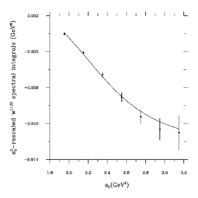
FIG. 5.: The rescaled $(1,3)$ spectral weight combination, $s_{0}^{3}\,J_{w^{(1,3)}}(s_{0})$ versus $s_{0}$. The integrals $J_{w^{(1,3)}}(s_{0})$ and errors were obtained using the ALEPH data and covariance matrix. The solid line shows the OPE prediction $f_{w^{(1,3)}}(\{a_{d}\};s_{0})$ corresponding to the combined fit of Eqs. (46).

FIG. 6.: $J_{w^{(k,m)}}(s_{0})$ and $f_{w^{(k,m)}}(\{a_{d}\};s_{0})$ for the $(0,0)$ (top left panel), $(1,0)$ (top right panel), $(1,1)$ (bottom left panel) and $(1,2)$ (bottom right panel) spectral weight pFESR’s. The $J_{w^{(k,m)}}(s_{0})$ integrals and errors were obtained using the ALEPH data and covariance matrix. The dashed and solid curves correspond to the OPE fit of DGHS, and our combined fit (Eqs. (46)), respectively.

FIG. 7.: $J_{w}(s_{0})$ and the corresponding MHA integrals for the $w_{1}$ (top left panel), $(0,0)$ (top right panel), $w_{3}$ (bottom left panel) and $(1,0)$ (bottom right panel) pFESR’s. The $J_{w}(s_{0})$ integrals and errors were obtained using the ALEPH data and covariance matrix.

FIG. 8.: $J_{w^{(k,m)}}(s_{0})$ and $f_{w^{(k,m)}}(\{a_{d}\};s_{0})$ for the $(3,1)$ (top panel) and $(4,0)$ (bottom panel) spectral weight pFESR’s. The $J_{w^{(k,m)}}(s_{0})$ integrals and errors were obtained using the ALEPH data and covariance matrix. The solid line shows the predictions based on the $d>4$ OPE solution represented by our combined fit, Eqs. (46).

REFERENCES

- [1] V. Cirigliano, J.F. Donoghue, E. Golowich and K. Maltman, Phys. Lett. B555, 71 (2003) [arXiv:hep-ph/0211420].
- [2] Y.S. Tsai, Phys. Rev. D4, 2821 (1971); H.B. Thacker and J.J. Sakurai, Phys. Lett. B36, 103 (1971); F.J. Gilman and D.H. Miller, Phys. Rev. D17, 1846 (1978); F.J. Gilman and S.H. Rhie, Phys. Rev. D31, 1066 (1985); E. Braaten, Phys. Rev. Lett. 60, 1606 (1988); S. Narison and A. Pich, Phys. Lett. B211, 183 (1988); E. Braaten, Phys. Rev. D39, 1458 (1989); S. Narison and A. Pich, Phys. Lett. B304, 359 (1993).
- [3] E. Braaten, S. Narison and A. Pich, Nucl. Phys. B373, 581 (1992).
- [4] F. Le Diberder and A. Pich, Phys. Lett. B286, 147 (1992) and B289, 165 (1992).
- [5] A. Pich, arXiv:hep-ph/9704453, in “Heavy Flavors II”, eds. A.J. Buras and M. Lindner, World Scientific, 1997.
- [6] W.J. Marciano and A. Sirlin, Phys. Rev. Lett. 61, 1815 (1988).
- [7] J. Erler, arXiv:hep-ph/0211345.
- [8] M. Davier, L. Girlanda, A. Höcker and J. Stern, Phys. Rev. D58, 096014 (1998) [arXiv:hep-ph/9802447].
- [9] M. Golterman, S. Peris, B. Phily and E. de Rafael, JHEP 0201:024 (2002) [arXiv:hep-ph/0112042].
- [10] S. Weinberg, Phys. Rev. Lett. 18, 507 (1967).
- [11] K. Maltman, Phys. Lett. B440, 367 (1998) [arXiv:hep-ph/9901239].
- [12] E. Poggio, H. Quinn and S. Weinberg, Phys. Rev. D13, 1958 (1976).
- [13] J.F. Donoghue and E. Golowich, Phys. Lett. B478, 172 (2000) [arXiv:hep-ph/9911309].
- [14] V. Cirigliano, J.F. Donoghue and E. Golowich, JHEP 0010, 048 (2000) [arXiv:hep-ph/0007196].
- [15] V. Cirigliano, J.F. Donoghue, E. Golowich and K. Maltman, Phys. Lett. B522, 245 (2001) [arXiv:hep-ph/0109113].
- [16] K. Maltman, arXiv:hep-ph/0209091.
- [17] M. A. Shifman, arXiv:hep-ph/0009131.
- [18] R. Barate et al. (The ALEPH Collaboration), Z. Phys. C76, 379 (1997); Eur. Phys. J. C4, 409 (1998).
- [19] K. Ackerstaff et al. (The OPAL Collaboration), Eur. Phys. J. C7, 571 (1999) [arXiv:hep-ex/9808019].
- [20] R. Barate et al., The ALEPH Collaboration, Eur. Phys. J. C11, 599 (1999) [arXiv:hep-ex/9903015].
- [21] M. Davier, S.M. Chen, A. Höcker, J. Prades and A. Pich, Nucl. Phys. Proc. Suppl. 98, 385 (2001).
- [22] M. Davier and C.Z. Yuan, arXiv:hep-ex/0211057.
- [23] Particle Data Group, K. Hagiwara et al., Phys. Rev. D66, 010001 (2002).
- [24] B.L. Ioffe and K.N. Zyablyuk, Nucl. Phys. A687, 437 (2001) [arXiv:hep-ph/0010089].
- [25] K.G. Chetyrkin and A. Kwiatkowski, Z. Phys. C59, 525 (1993) and arXiv:hep-ph/9805232.
- [26] K.G. Chetyrkin, J.H. Kuhn, A.A. Pivovarov, Nucl. Phys. B533, 473 (1998) [arXiv:hep-ph/9805335].
- [27] K. Maltman, Phys. Rev. D58: 093015 (1998) [arXiv:hep-ph/9804298]; A. Pich and J. Prades, JHEP 9806: 013 (1998) [arXiv:hep-ph/9804462].
- [28] K. Maltman and J. Kambor, Phys. Rev. D64: 093014 (2001) [arXiv:hep-ph/0107187].
- [29] S.C. Generalis, J. Phys. G15, L225 (1989); K.G. Chetyrkin, S.G. Gorishny and V.P. Spiridonov, Phys. Lett. B160, 149 (1990).
- [30] M. Gell-Mann, R.J. Oakes and B. Renner, Phys. Rev. 175, 2195 (1978).
- [31] G. Colangelo, J. Gasser and H. Leutwyler, Phys. Rev. Lett. 86, 5008 (2001) [arXiv:hep-ph/0103063].
- [32] A.A. Pivovarov, Yad. Fiz. 54, 1114 (1991) [Sov. J. Nucl. Phys. 54, 676 (1991)] and Z. Phys. C53, 461 (1992).
- [33] T. van Ritbergen, J.A.M. Vermaseren and S.A. Larin, Phys. Lett. B400, 379 (1997) [arXiv:hep-ph/9701390].
- [34] L.V. Lanin, V.P. Spiridonov and K.G. Chetyrkin, Yad. Fiz. 44, 1372 (1986) [Sov. J. Nucl. Phys. 44, 892 (1986)].
- [35] L.E. Adam and K.G. Chetyrkin, Phys. Lett. B329, 129 (1994) [arXiv:hep-ph/9404331].
- [36] M. Knecht, S. Peris and E. de Rafael, Phys. Lett. B508, 117 (2001) [arXiv:hep-ph/0102017].
- [37] A.J. Buras, M. Jamin, M.E. Lautenbacher and P.H. Weisz, Nucl. Phys. B400, 37 (1993) [arXiv:hep-ph/9211304].
- [38] J. Bijnens, E. Gamiz and J. Prades, JHEP 0110, 009 (2001) [arXiv:hep-ph/0108240].
- [39] J. Bijnens, E. Gamiz and J. Prades, arXiv:hep-ph/0209089.
- [40] S. Peris, B. Phily and E. de Rafael, Phys. Rev. Lett. 86, 14 (2001) [arXiv:hep-ph/0007338].
- [41] S. Narison, Nucl. Phys. B593, 3 (2001) [arXiv:hep-ph/0004247].
- [42] M. Knecht, Proc. Int. Conf. on High Energy Physics, HEP 2001, Budapest, Hungary, July 12-18, 2001.
- [43] M.A. Shifman, A.I. Vainshtein, and V.I. Zhakarov, Nucl. Phys. B147, 385, 448 (1979).
- [44] J. F. Donoghue, private communication.
- [45] A. Pich and J. Prades, JHEP 10, 004 (1999) [arXiv:hep-ph/9909244]; J.G. Korner, F. Krajewski and A.A. Pivovarov, Eur. Phys. J. C20, 259 (2001) [arXiv:hep-ph/0003165]; J. Kambor and K. Maltman, Phys. Rev. D62, 093023 (2000) [arXiv:hep-ph/0005156]; S. Chen, et al., Eur. Phys. J. C22, 31 (2001) [arXiv:hep-ph/0105253]; E. Gamiz, et al., JHEP 0301: 060 (2003) [arXiv:hep-ph/0212230].