Classical Gluodynamics of High Energy Nuclear Collisions: an Erratum and an Update

Abstract

We comment on the relation of our previous work on the classical gluodynamics of high energy nuclear collisions to recent work by Lappi (hep-ph/0303076). While our results for the non-perturbative number liberation coefficient agree, those for the energy disagree by a factor of 2. This discrepancy can be traced to an overall normalization error in our non-perturbative formula for the energy. When corrected for, all previous results are in excellent agreement with those of Lappi. The implications of the results of these two independent computations for RHIC phenomenology are noted.

I Introduction

In a series of recent papers, we computed numerically the classical gluodynamics of the early stages of very high energy nuclear collisions. These computations were first performed for an SU(2) Yang-Mills gauge theory AR99 ; AR00 ; AR01 and later for the SU(3) Yang-Mills gauge theory AYR01 ; AYR02a ; AYR02b . In a very recent paper, Lappi has independently performed the same computation for the SU(3) gauge theory Lappi . We will show that the apparent discrepancies in the two computations can be understood as arising from an incorrect overall normalization in the non-perturbative formula for the energy in our previous work. Since the problem arises from a normalization error, all of our previous results are still useful if interpreted appropriately. The purpose of this note is primarily to clarify the sources of discrepancy in the two computations and to present corrected results wherever necessary. Now that two independent computations can be shown to agree, we will show that they significantly constrain phenomenological interpretations of the RHIC data.

This note is organized as follows. In Section II, we discuss the different conventions for the small x classical effective Lagrangean density used in the literature and isolate the source of the normalization error in our previous computations. A reader uninterested in the details can skip right ahead to Section III where we discuss the corrected results for various quantities. The implications of these results for RHIC phenomenology are discussed in Section IV.

II Normalization of Classical Effective Lagrangean

There are two conventions for the classical effective Lagrangean density MV that are followed in the literature. This is occasionally confusing so we shall discuss these explicitly here. The first of these is

$$L_{I}[A,\rho]={1\over 4}\,F^{a}F^{a}-\rho^{a}A^{a}+i{\rho^{a}\rho^{a}\over 2\mu_{A}^{2}}\,.$$ (1)

For convenience, all Lorentz indices and space–time integrals have been suppressed here. For example, $F^{a}$ denotes the field strength tensor. In this form of the effective Lagrangean density, the coupling constant $g$ is absorbed in the definition of the charge density $\rho^{a}$. The color charge squared per unit area $\mu_{A}^{2}$ contains a factor $g^{2}$. The correlator of color charges is then

$$\langle\rho^{a}(x_{\perp})\rho^{a}(y_{\perp})\rangle=\mu_{A}^{2}\,\delta^{ab}\,\delta^{(2)}(x_{\perp}-y_{\perp})\,.$$ (2)

This form of the effective Lagrangean density is used in several works – for instance, Refs. KovMuell ; IancuMcLerran .

The other form of the effective Lagrangean density found in the literature, for instance in Refs. MV ; JKW ; GyulassyMcLerran is

$$L_{II}[A,\rho]={1\over 4}\,F^{a}F^{a}-g{\tilde{\rho}}^{a}A^{a}+i{{\tilde{\rho}}^{a}{\tilde{\rho}}^{a}\over 2\mu_{N}^{2}}\,.$$ (3)

Here $g$ is not absorbed in the definition of the charge density $\rho^{a}$ but appears explicitly in the second term of the classical effective Lagrangean density. The relation between the color charge squared values in the two Lagrangean densities is therefore

$$\mu_{A}^{2}=g^{2}\mu_{N}^{2}\,.$$

The form of the effective Lagrangean density in Eq. (3) is the form used in our papers AR99 ; AR00 ; AR01 ; AYR01 ; AYR02a ; AYR02b , and the scale we use, $\Lambda_{s}^{2}$ is defined to be $\Lambda_{s}^{2}=g^{4}\mu_{N}^{2}$. Eq. (1) of Ref. Lappi has the form

$$\langle\rho^{a}(x_{\perp})\rho^{a}(y_{\perp})\rangle=g^{2}\mu_{N}^{2}\,\delta^{ab}\,\delta^{(2)}(x_{\perp}-y_{\perp})\,.$$ (4)

Thus from Eqs. (2) and  (II), it is clear that the form of the effective Lagrangean density used by Lappi is Eq. (1), albeit with the color charge squared defined to be identical to ours.

In Eq. (1) and (3), the field strength tensor has the canonical form

$$F_{\mu\nu}^{a}=\partial_{\mu}A_{\nu}^{a}-\partial_{\nu}A_{\mu}^{a}+gf^{abc}A_{\mu}^{b}A_{\nu}^{c}\,.$$ (5)

In our numerical work – see for instance Ref. AR99 – the field strength tensor is defined as

$${{\overline{F}}}_{\mu\nu}^{a}=\partial_{\mu}{\overline{A}}_{\nu}^{a}-\partial_{\nu}{\overline{A}}_{\mu}^{a}+2f^{abc}{\overline{A}}_{\mu}^{b}{\overline{A}}_{\nu}^{c}\,.$$ (6)

Performing the field re-definition ${\overline{A}}_{\mu}^{a}={g\over 2}A_{\mu}^{a}$, we obtain

$${{\overline{F}}}_{\mu\nu}^{a}={g\over 2}\,F_{\mu\nu}^{a}\,.$$ (7)

The “canonical” effective Lagrangean density in Eq. (3) can then be re-written as

$$L_{II} = \left({2\over g}\right)^{2}\,\left({1\over 4}\,{{\overline{F}}}^{a}{{\overline{F}}}^{a}+{g^{2}\over 2}\,{\tilde{\rho}}^{a}{\overline{A}}^{a}\right)$$ (8)

$$+ i{{\tilde{\rho}}^{a}{\tilde{\rho}}^{a}\over 2\mu_{N}^{2}}\,.$$

With a further re-definition ${{\overline{\rho}}}^{a}=g^{2}{\tilde{\rho}}^{a}/2$, we obtain

$$L_{(II)} = {4\over g^{2}}\,\left({1\over 4}\,{\overline{F}}^{a}{\overline{F}}^{a}+{{\overline{\rho}}}^{a}{\overline{A}}^{a}\right)$$ (9)

$$+ i{{{\overline{\rho}}}^{a}{{\overline{\rho}}}^{a}\over 2\,g^{4}{\overline{\mu}}_{N}^{2}}\,,$$

where ${\overline{\mu}}_{N}=\mu_{N}/2$. With the field re-definition, $A^{a}\rightarrow A^{a}/g$, both $L_{I}$ and $L_{II}$, as defined in Eqs. (1) and (3) respectively, can be expressed in the same form as the right hand side of Eq. (9), albeit without the factor of $4$ in front of the first two terms, and with $\mu_{N}$ instead of ${\overline{\mu}}_{N}$. Since the continuum limit of the lattice Hamiltonian in Ref. Lappi corresponds to $L_{I}$ with $A^{a}\rightarrow A^{a}/g$ and $\rho^{a}={{\overline{\rho}}}^{a}/g$, there is this overall difference of a factor of 4 in the normalization between our lattice Hamiltonian and that of Lappi plus the requirement that the charge densities are related by ${\overline{\mu}}_{N}=\mu_{N}/2$.

Now consider the expression for the energy per unit rapidity per unit area,

$$\varepsilon\tau={1\over 2}\,\left(E^{a}E^{a}+B^{a}B^{a}\right)\,,$$ (10)

again suppressing Lorentz indices. From Eq. (7),

$${\overline{B}}^{a}={g\over 2}\,B^{a}\,\,\,;\,\,\,{\overline{E}}^{a}={g\over 2}\,E^{a}\,,$$ (11)

which gives

$$\varepsilon\tau={4\over g^{2}}\,{\overline{\varepsilon}}\tau\,.$$ (12)

In Refs. AR00 and  AYR01 , we computed

$${\overline{\varepsilon}}\tau={\overline{f}}_{E}\,\left(g^{2}{\overline{\mu}}_{N}\right)^{3}\,,$$ (13)

where ${\overline{f}}_{E}$ was determined by an extrapolation of the lattice results to the continuum limit. Then from Eq. (10) and (12), we obtain

$$\varepsilon\tau={4\over g^{2}}\,{\overline{f}}_{E}\,\left(g^{2}{\overline{\mu}}_{N}\right)^{3}\,.$$ (14)

However, ${\overline{\mu}}_{N}=\mu_{N}/2$. Performing this substitution, we obtain

$$\varepsilon\tau={1\over g^{2}}\,f_{E}\,\Lambda_{s}^{3}\,,$$ (15)

where $f_{E}={\overline{f}}_{E}/2$. Thus the physical value of the energy liberation coefficient is one half that computed previously. It accounts precisely for the result found by Lappi.

The number liberation coefficient remains the same after the field re-definitions. This is because the number per unit rapidity per unit area is defined to be

$$N={4\over g^{2}}{\overline{f}}_{N}\left(g^{2}{\overline{\mu}}_{N}\right)^{2}\,.$$ (16)

Since ${\overline{\mu}}_{N}=\mu_{N}/2$, this replacement here exactly cancels the extra factor of $4$ appearing in the normalization. Hence ${\overline{f}}_{N}=f_{N}$ – our previous result is in agreement with the result of Lappi.

The gluon number distributions in the two papers coincide if we replace $\Lambda_{s}\rightarrow\Lambda_{s}/2$. The resulting comparison of the result of Lappi to our prior result in Ref. AYR01 is excellent and is shown in Fig. 1.

III Corrected Results

Now that we understand the origin of the apparent discrepancies in the numerical results of Ref. Lappi and our prior results, we will discuss the corrected results here. As discussed previously AR00 , all dimensional quantities in the classical effective theory can be expressed in terms of the appropriate power of $\Lambda_{s}$ times a non-perturbative function of $\Lambda_{s}R$. This is because $\Lambda_{s}$ and $R$ are the only dimensional scales in the problem. $\Lambda_{s}$ is, in principle, a function of the energy, the centrality and the atomic number. For RHIC energies, one can broadly estimate that $\Lambda_{s}\sim 1$-2 GeV (more on this in the next section). The radius of a gold nucleus is approximately $6.5$ fm, so $\Lambda_{s}R$ lies in the range $32.5$ – $65$ for Au-Au collisions at RHIC. We obtain, for the transverse energy,

$${1\over\pi R^{2}}\,{dE_{T}\over d\eta}={f_{E}(\Lambda_{s}R)\over g^{2}}\,\Lambda_{s}^{3}\,.$$ (17)

Previously, in Ref. AYR01 , we had $f_{E}(25)=0.537$ and $f_{E}(83.7)=0.497$. Following Eq. (15), this should be corrected to read $f_{E}(50)=0.27$ and $f_{E}(167.4)=0.25$. The corresponding expression for the gluon number is

$${1\over\pi R^{2}}\,{dN\over d\eta}={f_{N}(\Lambda_{s}R)\over g^{2}}\,\Lambda_{s}^{2}\,,$$ (18)

with $f_{N}(50)=0.315$ and $f_{N}(167.4)=0.3$. The variation in the number with $\Lambda_{s}R$ is very small, on the order of 10%. These results are in good agreement with those of Lappi.

As we have explained in detail in our earlier papers, there are a variety of ways of defining the particle number for a generic field $\phi$ and its conjugate momentum $\pi$. Let us compare the results for the following three definitions (here and in the following $k_{T}$ is the transverse momentum of the field):

$$n(\vec{k}_{T}) = \sqrt{\langle|\phi(\vec{k}_{T})|^{2}\rangle\langle|\pi(\vec{k}_{T})|^{2}\rangle},$$ (19)

$$= \omega(\vec{k}_{T})\langle|\phi(\vec{k}_{T})|^{2}\rangle$$ (20)

$$= \langle|\pi(\vec{k}_{T})|^{2}\rangle/\omega(\vec{k}_{T}).$$ (21)

Here $\omega(\vec{k}_{T})$ is the eigenfrequency for a free massless plane wave of the wave number $\vec{k}_{T}$ on a square lattice. In our work, as in Lappi’s, these prescriptions are applied to field configurations in the Coulomb gauge. In Fig. 1 our transverse momentum distributions for gluons are compared with Lappi’s result. KNV I (circles) in Fig. 1 is the same distribution as in our previous papers, but with the correct value of $\Lambda_{s}$ used to set the horizontal scale. KNV I corresponds to the gluon number distribution from the definition Eq. (19),and $k_{T}$ dependence is extracted only for the transverse momenta along the principal lattice directions. The solid line is from Lappi’s numerical result, which is computed according to Eq. (21) using the entire Brillouin zone. KNV II is obtained by the same definition as Lappi’s and it is consistent. The deviation at large $k_{T}$ is considerd to be a consequence of how we define $k_{T}$ on the lattice. It should be noted that, with the lattice spacings used, the ultraviolet portion of the spectrum, $k_{T}/\Lambda_{s}\geq 3$, cannot reliably reproduce continuum physics.

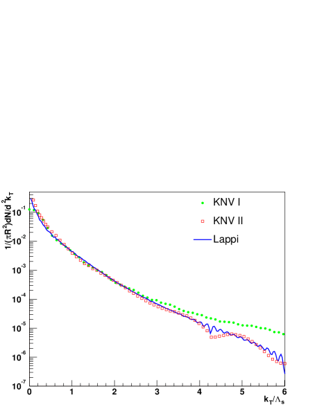
Figure 1: Comparison of gluon transverse momentum distributions per unit area as a function of $k_{T}/\Lambda_{s}$. KNV I (circles): the number defined as in Eq. (19), with $k_{T}$ taken to mean the lattice wave number along one of the principal directions. KNV II (squares) and Lappi (solid line): the number defined as in Eq. (21), with an average over the entire Brillouin zone and with $k_{T}$ taken to mean the frequency $\omega({\vec{k}}_{T})$.

The initial transverse energy per particle changes (because $f_{E}$ does) and is now

$${E_{T}\over N}=0.9\Lambda_{s}\,.$$ (22)

This value is nearly a factor of 2 lower than previously . As we will discuss in the following section, this lower value of the transverse energy per particle makes the connection to RHIC phenomenology simpler to interpret.

The “formation time” $\tau_{i}$ (defined as $\tau_{i}=1/\gamma(\Lambda_{s}R)/\Lambda_{s}$) of gluons extracted in Ref. AR00 (it is the same for SU(2) and SU(3) as confirmed in Ref. AYR01 ) is unaffected, albeit the $\Lambda_{s}R$ at which it is evaluated should be a factor of 2 larger than stated. One has approximately $\gamma=0.3$ in the range of interest. The initial energy density is then

$$\varepsilon={1\over\tau_{i}}\,{dE_{T}\over{\pi R^{2}d\eta}}={0.08\over g^{2}}\,\Lambda_{s}^{4}\,.$$ (23)

The number distributions, with coefficients appropriately scaled with $\Lambda_{s}$, have the same form as previously:

$${1\over\pi R^{2}}{dN\over d\eta d^{2}k_{T}}={1\over g^{2}}{\overline{f}}_{n}(k_{T}/\Lambda_{s})\,,$$ (24)

where ${\overline{f}}_{n}(k_{T}/\Lambda_{s})$ is

$${\overline{f}}_{n}=\left\{\begin{array}[]{ll}a_{1}\left[\exp\left(\sqrt{k_{T}^{2}+m^{2}}/T_{\rm eff}\right)-1\right]^{-1}&(k_{T}/\Lambda_{s}\leq 1.5)\\ \\ a_{2}\,\Lambda_{s}^{4}\log(4\pi k_{T}/\Lambda_{s})k_{T}^{-4}&(k_{T}/\Lambda_{s}>1.5)\\ \end{array}\right.$$ (25)

with $a_{1}=0.137$, $m=0.0358\Lambda_{s}$, $T_{\rm eff}=0.465\Lambda_{s}$, and $a_{2}=0.0087$.

With this expression for the number distributions, we can now compute the occupation number for gluons after the collision. The relevant quantity for the validity of the three dimensional classical approximation is the three dimensional occupation number  which can be estimated from the two dimensional boost-invariant number distribution computed in our simulation by the following relation MuellerQM2002 :

$$f^{\rm glue}={(2\pi)^{3}\over 2\,(N_{c}^{2}-1)}\,{1\over\pi R^{2}}\,{dN\over d\eta d^{2}\,k_{T}}\,.$$ (26)

Substituting our result for the number distribution from Eq. (19) here, one can compute the occupation number of gluons at the early stages of the collision. The results are shown in Fig. 2 for $\Lambda_{s}R=66$.

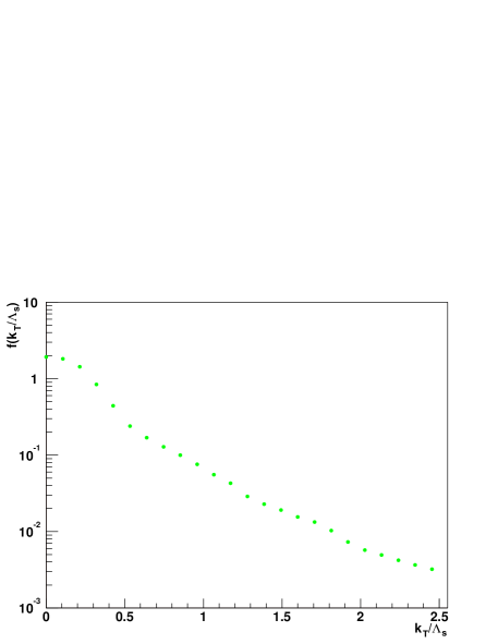
Figure 2: Gluon occupation number defined in Eq .(26), computed using Eq. (19).

Strictly speaking, the classical description is valid for $f>1$. It is not known however what the value of $f$ is at which the classical description breaks down completely and quantum corrections are dominant.

All of our other results can be understood by appropriate re-scaling. For instance, the $p_{t}$ distribution of the azimuthal asymmetry, $v_{2}(p_{t})$, plotted versus $p_{t}/\Lambda_{s}$ is the same after replacing $\Lambda_{s}\rightarrow\Lambda_{s}/2$ on the x-axis of the plot AYR02a . The peak in $v_{2}(p_{t})$ is therefore at even lower momenta then previously – at $p_{t}\sim\Lambda_{s}/8$.

IV Numerical Gluodynamics and RHIC Phenomenology

Now that we have shown that the results of two independent computations converge, it is useful to consider its implications for RHIC phenomenology. The results obtained in this classical approach are valid only at the very early stages of the nuclear collision and the connection to the final state distributions of measured hadrons might be considered remote. We will argue that, on the contrary, very general arguments can be applied to the RHIC data which will help constrain the properties of the initial state. In addition, they also significantly limit the freedom of final state interaction models which attempt to describe thermalization and the subsequent evolution of a Quark Gluon Plasma (QGP) in very high energy heavy ion collisions.

We know that the hadronic multiplicity at $\eta\approx 0$ for central Au-Au collisions with center of mass energy $\sqrt{s}=130$ GeV/nucleon at RHIC is $\sim 1000$ while the hadronic transverse energy is $\sim 500$ GeV experiment . One expects, on general grounds, the following relations, respectively, to hold for the transverse energy and the multiplicity:

$$E_{T}^{\rm glue} > E_{T}^{\rm hadrons}$$ (27)

$$N^{\rm glue} \leq N^{\rm hadrons}\,.$$ (28)

The inequality for the transverse energy follows from the expectation that some of the initial transverse energy is converted into work due to the expansion of the system MuellerQM2002 . Moreover, if the system were to approach thermalization due to re-scattering, this process would again cause the initial transverse energy to be transferred into longitudinal energy Mueller2000 . Even if there were no $pdV$ work done and no re-scattering, it is difficult to envision a scenario where the final transverse energy is larger than the initial one. The second constraint is also very plausible. For a thermal system, entropy is simply proportional to the multiplicity and the final entropy must be equal to or greater than the initial one. Even in the other extreme scenario, independent fragmentation with no re-scattering, parton-hadron duality suggests that the parton multiplicity prior to hadronization is equal to the multiplicity of hadrons after phd .

Combining the first condition in Eq. (28) on the transverse energy with Eq. (17) and the empirical result for the RHIC data, we find that

$$\Lambda_{s}^{\rm RHIC}>1.3\,\,{\rm GeV}\,.$$ (29)

Here we have assumed that the average transverse area for the range of impact parameters corresponding to the most central collisions is $\pi R^{2}=130$ fm² and $g=2$  Combining the second condition in Eq. (28) on the particle multiplicity (at $\eta=0$) with Eq. (18), we find

$$\Lambda_{s}^{\rm RHIC}\leq 2\,\,{\rm GeV}\,.$$ (30)

Also, from Eq. (22), and Eqs. (29)-(30), we obtain the following constraint for the initial transverse energy per particle:

$$1.14\,\,{\rm GeV}\leq{E_{T}\over N}_{\rm initial}^{\rm RHIC}\leq 1.76\,\,{\rm GeV}\,,$$ (31)

and, for the initial energy density, (from Eq. (23)),

$$7.1\,\,{\rm{GeV\over fm^{3}}}\leq\varepsilon_{\rm initial}^{\rm RHIC}\leq 40\,\,{\rm{GeV\over fm^{3}}}\,.$$ (32)

Thus the experimental data, the non-perturbative formulae in Eqs. (17)-(18) obtained from the classical numerical gluodunamics, and very general constraints can all be put together to significantly restrict the allowable range of $\Lambda_{s}^{\rm RHIC}$. These in turn restrict the initial transverse energy per particle and the initial energy density. How these quantities evolve tell us a great deal about the space-time evolution of partonic matter in a heavy ion collision.

In our analysis, $\Lambda_{s}$ is an external parameter – $\Lambda_{s}^{2}\equiv g^{4}\mu^{2}$, where $\mu^{2}$, as discussed previously, has the physical interpretation of being the average color charge squared per unit area per unit rapidity of color sources at higher values of $x$ than those of interest. This scale is not quite the same as the gluon saturation scale $Q_{s}^{2}$, which denotes the scale at which the gluon distribution changes qualitatively due to saturation effects KovMuell . The relation between the two can be obtained by comparing the analytical expressions for the gluon distributions in the two approaches JKMW ; Kovchegov ; KovMuell . One obtains AYR02b

$$Q_{s}^{2}\approx\Lambda_{s}^{2}\,{N_{c}\over 4\pi}\,\ln\left({\Lambda_{s}^{2}\over\Lambda_{QCD}^{2}}\right)\,.$$ (33)

For the values of $\Lambda_{s}$ in the range of interest, $Q_{s}\approx\Lambda_{s}$. Extrapolating the Golec-Biernat–Wusthoff parametrization to RHIC (with the appropriate $A^{1/3}$ dependence), we find $\Lambda_{s}^{2}\approx Q_{s}^{2}=2$ GeV². This value for $Q_{s}$ is also obtained by Kharzeev and Nardi KN . $\Lambda_{s}$ thus obtained lies within the range required by Eqs. (29) and Eq. (30). Nevertheless, there is an ambiguity in Eq. (33). For smaller values of $x$, one expects the infrared scale in this equation to be of order $Q_{s}$ and not $\Lambda_{QCD}$ KIIM ; Mueller ; the relation between $Q_{s}$ and $\Lambda_{s}$ will then be modified. Secondly, even at the classical level, the requirement that color neutrality be maintained Lam will alter the relation between $\Lambda_{s}$ and $Q_{s}$. Indeed, in this case, one can directly relate the two scales with an appropriate definition of $Q_{s}$. This point will be discussed further at a later date. Understanding this relation is important because the constraint on $\Lambda_{s}$ discussed here will translate into a constraint on the gluon content in the nuclei at RHIC energies.

The bounds in Eq. (31) and Eq. (32) are very important for understanding the “late” stage dynamics of high energy heavy ion collisions, namely, when the classical approach breaks down as it must. One possibility is that the system undergoes hydrodynamic expansion Rasanen . At the end of the classical stage , the system is completely out of equilibrium. This is because the momentum distribution is very anisotropic: $p_{t}\sim\Lambda_{s}$ and $p_{z}\sim 0$. If the system is to thermalize, there must be particle production after the classical stage. Particle number conserving $2\rightarrow 2$ interactions are too inefficient to thermalize the system within a reasonable time scale Mueller2000 ; BMSS . If $\Lambda_{s}$ is $2$ GeV, particles cannot be produced subsequent to the classical stage because this value saturates our bound for the particle number. If $\Lambda_{s}$ is $1.3$ GeV (at the lower end of our allowed range), one can certainly increase the particle number by approximately a factor of 2 after the classical stage. The transverse energy per particle (see Eq. (31)) will then also decrease by a commensurate amount and approach the experimental value. However, one cannot then have any hydrodynamic expansion (and therefore thermalization) because for $\Lambda_{s}=1.3$, the transverse energy was already as low as it could be: hydrodynamic expansion would lower it still further.

The problem with this “free streaming” scenario is that one does not have a satisfactory mechanism to explain the momentum dependence of the azimuthal anisotropy (especially at low $p_{t}$) observed at RHIC. The classical numerical simulations of $v_{2}$ do not generate enough $v_{2}$ AYR02a . There is an interesting attempt to explain the RHIC data as resulting from “non-flow” correlations but at low $p_{t}$ ($p_{t}<Q_{s}$) its energy dependence is different from the trend in the measured data from RHIC at $\sqrt{s}=130$ GeV/nucleon and $\sqrt{s}=200$ GeV/nucleon KovTuchin . A consistent picture of all the global features of the RHIC data might still be feasible within the straitjacket provided by the classical simulations and the data but there is limited room for models of final state interactions to maneuver.

- (1) A. Krasnitz and R. Venugopalan, hep-ph/9706329, hep-ph/9808332; Nucl. Phys. B557 237 (1999).
- (2) A. Krasnitz and R. Venugopalan, Phys. Rev. Lett. 84 (2000) 4309.
- (3) A. Krasnitz and R. Venugopalan, Phys. Rev. Lett. 86 (2001) 1717.
- (4) A. Krasnitz, Y. Nara and R. Venugopalan, Phys. Rev. Lett. 87, 192302 (2001).
- (5) A. Krasnitz, Y. Nara and R. Venugopalan, Phys. Lett. B 554, 21 (2003); arXiv:hep-ph/0209341.
- (6) A. Krasnitz, Y. Nara and R. Venugopalan, Nucl. Phys. A 717, 268 (2003).
- (7) T. Lappi, arXiv:hep-ph/0303076.
- (8) L. McLerran and R. Venugopalan, Phys. Rev. D49 2233 (1994); D49 3352 (1994); D50 2225 (1994).
- (9) Y. V. Kovchegov and A. H. Mueller, Nucl. Phys. B 529, 451 (1998).
- (10) E. Iancu, A. Leonidov and L. McLerran, arXiv:hep-ph/0202270; E. Iancu and R. Venugopalan, arXiv:hep-ph/0303204.
- (11) J. Jalilian-Marian, A. Kovner, A. Leonidov, and H. Weigert, Nucl. Phys. B504 415 (1997).
- (12) M. Gyulassy and L. McLerran, Phys. Rev. C56 (1997) 2219.
- (13) A. H. Mueller, arXiv:hep-ph/0208278.
- (14) . Adler et al. [STAR Collaboration], Phys. Rev. Lett. 87, 112303 (2001); K. Adcox et al. [PHENIX Collaboration], Phys. Rev. Lett. 87, 052301 (2001); I. G. Bearden et al. [BRAHMS Collaborations], Phys. Lett. B 523, 227 (2001); B. B. Back et al. [PHOBOS Collaboration], Phys. Rev. C 65, 061901 (2002).
- (15) K. J. Eskola, P. V. Ruuskanen, S. S. Rasanen and K. Tuominen, Nucl. Phys. A 696, 715 (2001).
- (16) A. H. Mueller, Nucl. Phys. B572 (2000) 227; J. Bjoraker and R. Venugopalan, Phys. Rev. C63 024609 (2001).
- (17) Ya. I. Azimov, Yu. L. Dokshitzer, V. A. Khoze, and S. I. Troyan, Z. Phys. C27:65, (1985).
- (18) J. Jalilian–Marian, A. Kovner, L. McLerran and H. Weigert, Phys. Rev. D55 5414 (1997).
- (19) Y. V. Kovchegov, Phys. Rev. D 54, 5463 (1996).
- (20) D. Kharzeev and M. Nardi, Phys. Lett. B 507, 121 (2001); D. Kharzeev and E. Levin, Phys. Lett. B 523, 79 (2001); D. Kharzeev, E. Levin and M. Nardi, arXiv:hep-ph/0111315.
- (21) E. Iancu, K. Itakura and L. McLerran, Nucl. Phys. A 708, 327 (2002).
- (22) A. H. Mueller, arXiv:hep-ph/0206216.
- (23) C. S. Lam and G. Mahlon, Phys. Rev. D 61, 014005 (2000); ibid., 62, 114023 (2000).
- (24) R. Baier, A. H. Mueller, D. Schiff and D. T. Son, Phys. Lett. B502 51 (2001); B539, 46 (2002).
- (25) Y. V. Kovchegov and K. L. Tuchin, Nucl. Phys. A 708, 413 (2002).