Abstract

Neutrino Oscillation, in which a given flavour of neutrino transforms into another is a powerful tool for probing small neutrino masses. The intrinsic neutrino properties involved are neutrino mass squared difference $\Delta m^{2}$ and the mixing angle in vacuum $\theta$. In this talk I will summarize the progress that we have achieved in our search for neutrino oscillation with special emphasis on the recent results from the Sudbury Neutrino Observatory (SNO) on the measurement of solar neutrino fluxes. I will outline the current bounds on the neutrino masses and mixing parameters and discuss the major physics goals of future neutrino experiments in the context of the present picture.

1 Introduction

Since it was proposed in 1929 by Pauli the question whether neutrinos are massive or not has been an intriguing issue. The Standard Model (SM) contains only massless neutrinos in left handed doublets. But there is no fundamental principle like the gauge invariance which makes the photon massless –that would forbid a mass term for the neutrinos. Most extensions of the SM predict small but non-zero neutrino masses. A non-zero neutrino mass would not only constitute a signal of physics beyond standard model it would also help in probing the underlying gauge symmetry governing the interactions. Moreover because of the important role played by neutrinos in stellar evolution, supernova dynamics, nucleosynthesis and structure formation in the early universe the implications of massive neutrinos can be very significant for astrophysics and cosmology.

Direct bounds on neutrino masses are obtained from purely kinematical measurements
$\bullet$ $m_{\nu_{e}}<$ 2.2 eV (${}^{3}{H}\rightarrow^{3}{He}+e^{-}+\bar{\nu_{e}}$) [1]
$\bullet$ $m_{\nu_{\mu}}<$ 170 KeV (Pion decay) [2]
$\bullet$ $m_{\nu_{\tau}}<$ 15.5 MeV (Tau decay) [3].
A bound on the effective mass of the electron neutrino can be obtained from the absence of the neutrinoless double beta decay process which gives $\langle{m_{ee}}\rangle\equiv|\sum U_{ei}^{2}m_{\nu_{i}}|\leq 0.38p$ eV at 95%  CL, where $p\sim 0.6-2.8$ denotes the uncertainty in nuclear matrix element [4]. $U$ is the neutrino mixing matrix and $m_{\nu_{i}}(i=1,2,3)$ denote the neutrino mass values. This process is lepton number violating and the occurrence of such an event would indicate that neutrinos are Majorana fermions i.e. their own antiparticles. An important bound on neutrino mass comes from cosmology

$$\sum_{i}m_{\nu_{i}}<100h^{2}{\rm eV}$$ (1)

which implies masses much smaller than the kinematical bounds.

Very small neutrino mass squared differences can be probed by neutrino oscillation which arises if neutrinos have mass and different flavours mix among themselves. Thanks to painstaking experimental efforts we now have strong evidences in favour of neutrino oscillation coming from the measurement of solar and atmospheric neutrino fluxes. The high statistics SuperKamiokande(SK) and SNO experiments have established the conjecture of neutrino flavour conversion as a reality and provided important information on neutrino mass and mixing. The purpose of this talk is to discuss the recent developments in the neutrino oscillation experiments and the bounds on neutrino mass squared differences and mixing angles obtained from these. Since the results and implications of the SK experiment has been discussed in detail by Mark Vagins in these proceedings the emphasis on this paper will be on the recent SNO results. In section 2 we develop briefly the formalism for neutrino oscillation in vacuum as well as in matter. In section 3 we discuss the neutrino oscillation experiments and discuss the constraint that one obtains on $\Delta{m}^{2}$ and $\theta$ from two and three generation oscillation analyses. In section 4 we discuss if the current data requires a fourth sterile neutrino or not. In section 5 we discuss the goals and salient features of the future experiments which are soon expected to give data/start operation. Finally we present the concluding remarks.

2 Neutrino Oscillation In Vacuum

We consider a neutrino flavor state $|{\nu_{\alpha}}>$ created in weak interaction processes. In general this is a superposition of neutrino mass eigenstates $|\nu_{i}>$

$$|\nu_{\alpha}>=\Sigma_{i}U_{\alpha i}|\nu_{i}>$$ (2)

where $U$ is the unitary mixing matrix analogous to the Cabibbo-Kobayashi-Maskawa matrix in the quark sector. Assuming ultra-relativistic neutrinos with a common definite momentum $p$, $E_{i}\simeq p+{m_{i}^{2}}/{2p}$i, $U$ to be real i.e. neglecting CP violating phases in the lepton sector the probability that a neutrino of flavour $\alpha$ gets converted to a neutrino of flavour $\beta$ after traversing a distance $L$ is

$$P(\nu_{\alpha},0;\nu_{\beta},t)=\delta_{\alpha\beta}-4~{}\Sigma_{j>i}~{}U_{\alpha i}U_{\beta i}U_{\alpha j}U_{\beta j}\sin^{2}\left(\frac{\pi L}{\lambda_{ij}}\right)$$ (3)

where $\lambda_{ij}$ is defined to be the neutrino vacuum oscillation wavelength given by,

$$\lambda_{ij}=(2.47{\rm m})\left(\frac{E}{MeV}\right)\left(\frac{\Delta_{ij}}{eV^{2}}\right)^{-1}$$ (4)

which denotes the scale over which neutrino oscillation effects can be significant;
$\Delta_{ij}=\mid{m_{j}^{2}-m_{i}^{2}}\mid$. The oscillatory character is embedded in the $\sin^{2}(\frac{\pi L}{\lambda_{ij}})$ term. If $\Delta_{ij}$ is such that the corresponding $\lambda_{ij}>>L$, the oscillatory term $\sin^{2}{\pi L/\lambda_{ij}}\rightarrow 0$, whereas $\lambda_{ij}<<L$ would imply a large number of oscillations and consequently the $\sin^{2}{\pi L/\lambda_{ij}}$ term averages out to 1 /2, when integrated over energy and/or source /detector position.
For two-generations, $U$ can be parametrised by a single mixing angle $\theta$ as:

$$U=\pmatrix{\cos{\theta}&\sin{\theta}\cr-\sin{\theta}&\cos{\theta}\cr}$$ (5)

and the conversion probability is

$$P_{\nu_{\alpha}\nu_{\beta}}=\sin{{}^{2}}2\theta\sin{{}^{2}}(1.27{\Delta m}^{2}L/E)$$ (6)

where $\Delta{m}^{2}$ is in eV², $L$ is in meters and $E$ is in MeV. From the above equation we see that oscillation effect is maximum for $\mbox{$\Delta{m}^{2}$~{}}\sim L/E$. Consequently the values of $\Delta{m}^{2}$ that can be explored in an experiment depend on the energy of the neutrino beam and the source-detector distance. Table 1 shows the typical $L/E$ and the $\Delta{m}^{2}$ that can be probed in various experiments using different neutrino sources. Since the energy usually has a spread, each experiment is actually sensitive to a range of $\Delta{m}^{2}$ .

3 Matter-Enhanced Resonant Flavor Conversion

Wolfenstein and later Mikheyev and Smirnov [5] pointed out that interaction of the neutrinos with matter modifies their dispersion relation and consequently they develop an effective mass dependent on the matter density. For unpolarized electrons at rest, the forward charged current scattering of neutrinos off electron gives rise to an effective potential

$$V_{cc}=\sqrt{2}G_{F}n_{e}$$ (7)

while the neutral current interaction gives a contribution (assuming charge neutrality)

$$V_{nc}=-\sqrt{2}G_{F}n_{n}/2$$ (8)

Experiment	Energy(E)	Distance(L)	$\Delta m^{2}$
Reactor	1 MeV	100m	$10^{-2}$ eV2
Low Energy	10 MeV	100m	$10^{-1}$ eV2
Accelerator
High Energy	1 GeV	1 km	1 eV2
Accelerator
Atmospheric	1 GeV	10,000 km	$10^{-4}$ eV2
Neutrinos
Solar Neutrinos	10 MeV	$10^{11}$ m	$10^{-10}$ eV2
Long-Baseline	1 MeV	1 km	$10^{-3}$ eV 2
Reactor
Long-Baseline	1 GeV	1000km	$10^{-3}$ eV2
Accelerator

Table 1: Sensitivity to $\Delta m^{2}$ in various oscillation experiments for vacuum mixing

Considering for simplicity two neutrino flavours $\nu_{e}$ and $\nu_{\mu}$ the neutrino propagation equation in flavour basis in the presence of matter is

$${i\frac{d}{dt}{\pmatrix{\nu_{e}\cr\nu_{\mu}\cr}}={M_{F}}{\pmatrix{\nu_{e}\cr\nu_{\mu}\cr}}}$$ (9)

$$M_{F}={U}\pmatrix{m_{1}^{2}/2E&0\cr 0&m_{2}^{2}/2E\cr}U^{\dagger}+EI\\ \\ \\ +\pmatrix{{\sqrt{2}G_{F}n_{e}}&0\cr 0&0\cr}-{\frac{G_{F}n_{n}}{\sqrt{2}}}I$$ (10)

The last two terms denote the matter contribution. The terms proportional to the identity matrix contributes to the overall phase and dropping these terms the mass matrix in flavour basis takes the form

$$M_{F}=\frac{1}{2E}{\pmatrix{\Delta m^{2}sin^{2}\theta+{2\sqrt{2}G_{F}n_{e}E}&\Delta m^{2}sin2\theta\cr\Delta m^{2}sin2\theta&\Delta m^{2}cos^{2}\theta\cr}}$$ (11)

$\Delta m^{2}=m_{2}^{2}-m_{1}^{2}$. The mass eigenvalues in matter is obtained by diagonalizing the above matrix. The flavour and mass states in matter are now related as

$$\pmatrix{{\nu_{e}}\cr\nu_{\mu}\cr}=\pmatrix{cos\theta_{M}&sin\theta_{M}\cr-sin\theta_{M}&cos\theta_{M}\cr}\pmatrix{\tilde{\nu_{1}}\cr\tilde{\nu_{2}}\cr}$$ (12)

where the mixing angle in matter is given as

$$\tan 2\theta_{M}=\frac{\Delta m^{2}\sin 2\theta}{\Delta m^{2}\cos 2\theta-2\sqrt{2}G_{F}n_{e}E}$$ (13)

$n_{e}$ is the electron density of the medium and $E$ is the neutrino energy. Eq. (13) demonstrates the resonant behavior of $\theta_{M}$. Assuming $\Delta m^{2}>0$ the mixing angle in matter is maximal (irrespective of the value of mixing angle in vacuum) for an electron density satisfying,

$$2\sqrt{2}G_{F}n_{e,res}E=\Delta m^{2}\cos 2\theta$$ (14)

This is the Mikheyev-Smirnov-Wolfenstein (MSW) effect of matter-enhanced resonant flavor conversion.

4 Oscillation Experiments

Experimental searches for neutrino oscillation can be classified into two categories
$\bullet$ Disappearance Experiment – in which one looks for the diminution of the neutrino flux due to oscillation to some other flavor to which the detector is not sensitive.
$\bullet$ Appearance Experiment – in which one looks for a new neutrino flavor not present in the initial beam, which can arise from oscillation.

4.1 Reactor And Accelerator Neutrino Experiments

Nuclear reactors provide an intense source of  $\overline{\nu_{e}}$ with energies $\sim$ 1 MeV. Because of this low energy spectrum, reactor based oscillation experiments are suitable for searching for $\overline{\nu_{e}}$ going to any flavor using disappearance technique. The dominant systematic uncertainties come from the strength of the neutrino source, the detector efficiency, the cross-section for neutrino interactions etc. These limit the sensitivity of the mixing angle that can be probed in these experiments. The systematic uncertainties are largely eliminated when energy spectra measured at two different detector positions are compared.

There are two types of accelerator neutrino beams. Low-energy accelerators (the Meson-factories) provide an equal admixture of $\nu_{\mu}$, $\nu_{\bar{\mu}}$ and $\nu_{e}$ from decays of stopped $\pi^{+}$ and $\mu^{+}$. These are of energy $\sim$ 10 MeV. High-energy accelerators produce $\nu_{\mu}$ (${\bar{\nu_{\mu}}}$) beams coming from K or $\pi$ decay, the $\nu_{e}$ component being small. The mean energy of these type of neutrinos are $\sim$ 1 GeV. These are suitable to look for ${\nu_{\mu}}$ (${\bar{\nu_{\mu}}}$) $\rightarrow{\nu_{e}}$ (${\bar{\nu_{e}}}$) or ${\nu_{\mu}}$ (${\bar{\nu_{\mu}}}$) $\rightarrow{\nu_{\tau}}$ (${\bar{\nu_{\tau}}}$) by appearance method or to measure the probability of ${\nu_{\mu}}$ (${\bar{\nu_{\mu}}}$) $\rightarrow$ ${\nu_{\mu}}$ (${\bar{\nu_{\mu}}}$) by disappearance technique. For the appearance experiments one needs to understand the backgrounds thoroughly in order to identify an event arising from oscillation. Table 2 shows the characteristics of some of the important reactor and accelerator based experiments.

		probes	signal
	experiment	oscillation	for	$\Delta{m}^{2}$ in eV2	$\sin^{2}2\theta$
		channel	oscillation
	GÖSGEN	${\nu_{e}}\rightarrow\nu_{x}$	negative	$<0.02$	$<0.02$
	Krasnoyarsk	${\nu_{e}}\rightarrow\nu_{x}$	negative	$<0.014$	$<0.14$
$I$	BUGEY	${\nu_{e}}\rightarrow\nu_{x}$	negative	$<0.01$	$<0.2$
	CHOOZ	${\nu_{e}}\rightarrow\nu_{x}$	negative	$<0.002$	$<0.1$
	Palo Verde	${\nu_{e}}\rightarrow\nu_{x}$	negative	$<0.002$	$<0.6$
	CDHSW	${\nu_{\mu}}\rightarrow\nu_{x}$	negative	$<0.23$	$<0.02$
	CHARM	${\nu_{\mu}}\rightarrow\nu_{x}$	negative	$<0.29$	$<0.2$
	CCFR	${\bar{\nu_{\mu}}}\rightarrow\bar{\nu}_{x}$	negative	$<15$	$<0.02$
	E776	${\bar{\nu_{\mu}}}\rightarrow\bar{\nu}_{x}$	negative	$<0.075$	$<0.003$
	E531	${\nu_{\mu}}\rightarrow{\nu_{\tau}}$	negative	$<0.9$	$<0.004$
$II$	E531	${\nu_{e}}\rightarrow{\nu_{\tau}}$	negative	$<9$	$<0.12$
	LSND	${\bar{\nu_{\mu}}}\rightarrow{\bar{\nu_{e}}}$	positive
	LSND	${\nu_{\mu}}\rightarrow{\nu_{e}}$	positive	} 1.2	}0.003
	KARMEN2	${\bar{\nu_{\mu}}}\rightarrow{\bar{\nu_{e}}}$	negative	$<0.007$	$<0.0021$

Table 2: The major reactor (I) and accelerator (II) experiments that are running/completed. From ref. [9].

With the exception of the LSND experiment all the reactor and accelerator based experiments of Table 2 are seen to consistent with no neutrino oscillation and provide exclusion regions in the $\Delta{m}^{2}$ - $\sin^{2}2\theta$ parameter space. In Table 2 We display the minimum value of $\Delta{m}^{2}$ and minimum value of $\sin^{2}2\theta$ that are excluded by the experiments that observe null oscillations. The LSND collaboration [6] gives $P_{\overline{\nu}_{\mu}\overline{\nu}_{e}}$ of $({0.31}^{+0.11}_{-0.10}\pm 0.05)$% corroborating their earlier result. They have also looked for $\nu_{\mu}-\nu_{e}$ oscillations. This gives an oscillation probability of $(0.26\pm 0.1\pm 0.05)$%. However a similar experiment KARMEN at the Rutherford laboratories searching for ${\bar{\nu_{\mu}}}-{\bar{\nu_{e}}}$ oscillations did not find any evidence of oscillation [7]. Combining the positive result of LSND with the no-oscillation result from KARMEN, the earlier ${\bar{\nu_{\mu}}}-{\bar{\nu_{e}}}$ experiment E776 at BNL [8], and the reactor experiment Bugey results in a very narrow range of allowed $\Delta{m}^{2}$ from 0.4 - 2 $eV^{2}$ at 95% C.L..

4.2 Atmospheric Neutrinos

The primary components of the cosmic-ray flux interact with the earth’s atmosphere producing pions and kaons which can decay as:

$\pi^{\pm}(K^{\pm})\rightarrow\mu^{\pm}+\nu_{\mu}(\overline{\nu}_{\mu})$

$\mu^{\pm}\rightarrow e^{\pm}+\nu_{e}(\overline{\nu}_{e})+$

From this decay chain one expects the number of muon neutrinos to be about twice that of electron neutrinos and as many neutrinos as antineutrinos. Atmospheric neutrino fluxes have been computed by several authors [10, 11]. Due to uncertainties arising from the primary cosmic ray spectrum, its composition, the hadronic interaction cross-sections, etc. different computations of the absolute ${\nu_{e}}~{}+{\bar{\nu_{e}}}$  and ${\nu_{\mu}}~{}$+ ${\bar{\nu_{\mu}}}$  fluxes agree only within 20-30%.

Measurement of atmospheric neutrino flux has been carried out using two different techniques: by imaging water $\breve{\rm C}$erenkov detectors, – Kamiokande [12] and IMB [13] – or using iron calorimeters as is done in Fréjus [14], Nusex [15] and Soudan2 [16]. To reduce the uncertainty in the absolute flux values these groups presented the double ratios $R$

$$R={\frac{(\nu_{\mu}+\overline{\nu}_{\mu})/(\nu_{e}+\overline{\nu}_{e})_{\rm obsvd}}{(\nu_{\mu}+\overline{\nu}_{\mu})/(\nu_{e}+\overline{\nu}_{e})_{\rm MC}}}$$ (15)

where MC denotes the Monte-Carlo simulated ratio. Different calculations agree to within better than 5% on the magnitude of this quantity. The value of R was found to be less than the expected value of unity in Kamiokande, IMB and Soudan2. This discrepancy came to be known as the atmospheric neutrino problem and an explanation to this was sought in terms of neutrino oscillations. The results from the high statistics SuperKamiokande experiment not only confirmed this but also provided an independent and strong evidence in favour of neutrino oscillation and hence neutrino mass from the measurement of the zenith angle dependence of the data. The SK data indicate a deficit of the muon-neutrinos passing upward through the earth ($\theta_{zenith}>90^{o}$). For the downward muon neutrinos ($\theta_{zenith}<90^{o}$) no such deficit was found. For electron neutrino events the ratio $N_{up}/N_{down}$ was found to consistent with expectations. A convincing explanation of all aspects of SK data comes in terms of $\nu_{\mu}-\nu_{\tau}$ oscillation. The 1289 day SK data [17] give $\sin^{2}2\theta>0.88$ and $1.6\times 10^{-3}$ eV${}^{2}<\Delta m^{2}<4\times 10^{-3}$ eV² at 90% C.L.. Pure $\nu_{\mu}-\nu_{s}$ oscillation is disfavoured at 99% C.L.. The charged current data from SK looking for $\nu_{\tau}$ interactions is reported to be consistent with $\nu_{\tau}$ appearance at 2$\sigma$ level [18].

5 Solar Neutrinos

The sun is a copious source of electron neutrinos, produced in the thermonuclear reactions that generate solar energy. The underlying nuclear process is:

$$4\;p\;\;\rightarrow\;\alpha\;+\;2\;e^{+}\;+\;2\;\nu_{e}\;+\;25\;{\rm MeV}$$

The above reaction is the effective process driven by a cycle of reactions (e.g. the $pp$-chain or the CNO cycle). Neutrinos are produced in several stages and those from a particular reaction have a characteristic spectrum. The solar neutrino fluxes are calculated using Standard Solar Models (SSM) the most popular among these are the ones due to Bahcall and his collaborators [19].

5.1 Solar Neutrino Experiments

So far seven experiments have published results on measurements of solar neutrino flux.
$\bullet$ Radiochemical Detectors

The pioneering experiment is the Cl experiment at Homestake which employs the reaction [20]

$$\nu_{e}+^{37}{Cl}\rightarrow^{37}{Ar}+e^{-}.$$ (16)

for detecting the neutrinos. The threshold is 0.814 MeV and is sensitive to the ${}^{8}{B}$ and ${}^{7}{Be}$ neutrinos.

Three experiments SAGE in Russia and GALLEX and GNO (upgraded version of GNO) in Gran Sasso underground laboratory in Italy employ the following reaction [21]

$$\nu_{e}\;+\;^{71}Ga\;\rightarrow\;^{71}Ge\;+\;e^{-}$$ (17)

This reaction has a low threshold of 0.233 MeV and the detectors are sensitive to the basic $pp$ neutrinos. Since the $pp$-chain is mainly responsible for the heat and light generation in the sun, detection of these neutrinos constitute an important step towards establishment of the accepted ideas of solar energy synthesis.
$\bullet$ $\breve{\rm C}$erenkov Detectors

The water $\breve{\rm C}$erenkov detector KamioKande in Japan detected the $\breve{\rm C}$erenkov light emitted by electrons which are scattered in the forward direction by solar neutrinos

$$\nu_{x}~{}+~{}e\rightarrow~{}\nu_{x}~{}+~{}e.$$ (18)

In addition to $\nu_{e}$ this reaction is also sensitive to $\nu_{\mu}$ and $\nu_{\tau}$ though with a reduced strength. Since Kamiokande’s energy threshold (for the recoil electron) was 7.5 MeV, it could measure only the ${}^{8}{B}$ neutrino flux. But one of the most important aspect was from a reconstruction of the incoming neutrino track it for the first time verified that the neutrinos are indeed of solar origin [22]. The KamioKande is upgraded to SuperKamiokande which started taking data from 1996. It has so far provided 1496 days of data [23].

The most recent results on solar neutrino flux measurement has come from the heavy water $\breve{\rm C}$erenkov detector at Sudbury Neutrino Observatory [24]. There are three reactions which are used by this experiment
$\nu_{e}+d\rightarrow p+p+e$        (CC)
$\nu_{x}+e\rightarrow\nu_{x}+e$            (ES)
$\nu_{x}+d\rightarrow p+n+\nu_{x}$      (NC)
The CC and ES reactions have a threshold of 5 MeV for the recoil electron while for NC the neutrino energy threshold is s 2.2 MeV. Thus these reactions are sensitive only to the ${}^{8}{B}$ neutrinos. The NC reaction is sensitive to all neutrino flavours with equal strength and thus provides a direct model independent evidence of the total solar ${}^{8}{B}$ flux.

In Table 3 we present the fluxes observed in these experiments with respect to the SSM predictions. The observed fluxes in all the experiments are less than the expectations from SSM and this constitutes the essence of the solar neutrino problem.

experiment	$R$	composition
$Ga$	0.584 $\pm$ 0.039	$pp(55\%),Be(25\%),B(10\%)$
$Cl$	0.335 $\pm$ 0.029	$B(75\%),Be(15\%)$
$SK$	0.459 $\pm$ 0.017	$B(100\%)$
$SNO(CC)$	0.349 $\pm$ 0.021	$B(100\%)$
$SNO(ES)$	0.473 $\pm$ 0.074	$B$ (100%)

Table 3: The observed solar neutrino rates relative to the $SSM$ predictions [19] are shown along with their compositions for different experiments.

However as more and more data accumulated it became more focused. If we combine the ${}^{8}{B}$ flux observed in SK with the Cl experimental rate, it shows a strong suppression of the ${}^{7}{Be}$ neutrinos. The pp flux constrained by solar luminosity along with the ${}^{8}{B}$ flux observed in SK leaves no room for the ${}^{7}{Be}$ neutrinos in Ga. This vanishing of the ${}^{7}{Be}$ neutrinos renders a purely astrophysical solution to the solar neutrino problem impossible and neutrino flavour conversion was conjectured as a plausible solution. This was beautifully confirmed by the SNO data. The ${}^{8}{B}$ flux measured by the CC and ES reactions in SNO is

$\Phi_{CC}^{SNO}=1.75\pm 0.07(stat)^{+0.12}_{-0.11}(sys)\times 10^{6}cm^{-2}s^{-1}$

$\Phi_{ES}^{SNO}=2.39\pm 0.34(stat)^{+0.16}_{-0.14}(sys)\times 10^{6}cm^{-2}s^{-1}$

The later is consistent with that observed by the SuperKamiokande (SK) detector [25] via the same reaction

$\Phi_{ES}^{SK}=2.32\pm 0.03(stat)^{+0.08}_{-0.07}\times 10^{6}cm^{-2}s^{-1}$

Since the CC reaction is sensitive only to $\nu_{e}$ and the ES reaction is sensitive to both $\nu_{e}$ and $\nu_{\mu}/\nu_{\tau}$ a higher ES flux would signify the presence of $\nu_{\mu}/\nu_{\tau}$. The combination of SNO CC and SK ES data provides a 3.3$\sigma$ signal for $\nu_{e}$ transition to an active flavour (or against $\nu_{e}$ transition to solely a sterile state). The total flux of active ${}^{8}{B}$ neutrinos determined from these measurements is $5.44\pm 0.99\times 10^{6}cm^{-2}s^{-1}$ which is in close agreement with the SSM value [19].

SNO has also published data on the CC spectrum and it gives a flat spectrum consistent with the flat recoil electron spectrum observed at SK. This is in contrast with the strong energy dependence observed by the data on total rates. Apart from the total fluxes, SK has also provided the fluxes measured at day and night. The day-night flux difference observed at SK :

$$\frac{D-N}{(D+N)/2}=-0.034\pm 0.022\pm 0.013$$

which is a $1.3\sigma$ effect. As we will see in the next section all these different aspects of the solar neutrino data contribute in shaping up the allowed areas in $\Delta m^{2}-\tan^{2}\theta$ plane.

5.2 Bounds on Neutrino mass and mixing including the SNO CC data

In this section I present the allowed regions in neutrino mass and mixing parameters by performing a global and unified $\chi^{2}$ analysis of the solar neutrino data including the SNO CC rate.

5.2.1 Two generation $\nu_{e}-\nu_{active}$ analysis

The general expression for $\nu_{e}$ survival probability in an unified formalism over the mass range $10^{-12}-10^{-3}$ eV² and for the mixing angle $\theta$ in the range [0,$\pi/2$] is [26]

$$P_{ee} = P_{\odot}P_{\oplus}+(1-P_{\odot})(1-P_{\oplus})$$ (19)

$$+2\sqrt{P_{\odot}(1-P_{\odot})P_{\oplus}(1-P_{\oplus})}\cos\xi$$

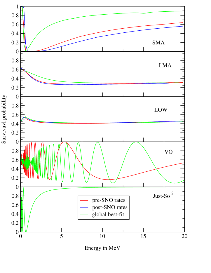
Figure 1: $P_{ee}$ vs. Energy at the best-fit values obtained from rates and rates+spectrum analysis

where $P_{\odot}$ denotes the probability of conversion of $\nu_{e}$ to one of the mass eigenstates in the sun and $P_{\oplus}$ gives the conversion probability of the mass eigenstate back to the $\nu_{e}$ state in the earth. All the phases involved in the Sun, vacuum and inside Earth are included in $\xi$. This most general expression reduces to the well known MSW (the phase $\xi$ is large and averages out) and vacuum oscillation limit (matter effects are absent and the phase $\xi$ is important) for appropriate values of $\Delta m^{2}/E$. The procedure which we use for calculating $P_{\oplus}$ and $P_{\odot}$ in MSW, vacuum as well as the in-between quasi-vacuum (QVO) regions where both $\xi$ and matter effects are relevant is discussed in [27]. We present in Table 4 the results of the $\chi^{2}$ analysis for ${\nu_{e}}-\nu_{\rm active}$ oscillations for only rates analysis as well as for global analysis including both rate and SK spectrum data. We use data from the Cl, Ga, SK and SNO experiments as given in Table 3 and the 1258 day SK recoil electron energy spectrum at day and night . We show the best-fit values of the parameters $\Delta{m}^{2}$ and $\tan^{2}\theta$, $\chi^{2}_{\rm min}$ and the goodness of fit (GOF) for the small mixing angle (SMA), large-mixing angle (LMA), LOW-QVO (low $\Delta{m}^{2}$ -quasi-vacuum), vacuum oscillation (VO) and Just So² solutions. The best-fit for the only rates analysis comes in the VO region which is favored at 28.79%. For the global rates + spectrum analysis we get five allowed solutions LMA, VO, LOW, SMA and Just So² in order of decreasing GOF. Best-fit comes in the LMA region. In fig. 1 we plot the probabilities vs. energy for this five solutions at the best-fit values obtained from only rates and rates+spectrum analysis. The LMA and the LOW solution can reproduce the flat recoil electron spectrum observed at SK well and hence from the global rate and spectrum analysis LMA and LOW are preferred. For the VO solution at the best-fit values from only rates analysis there is a non-monotonic dependence on energy which explains the rates data well. However the spectrum data requires a flat energy spectrum and the best-fit shifts to $\sim 4.5\times 10^{-10}$ eV². For the SMA solution also there is a mismatch between the parameters that give the minimum $\chi^{2}$ for the rates data and the spectrum data. The spectrum data prefers value of $\tan^{2}\theta$ which is one order of magnitude lower than that preferred by the rates data. This conflict increases with the inclusion of the SNO CC rate as is seen from fig. 1 where we plot the probabilities for the SMA region at best-fit values of pre-SNO and post-SNO rate analysis. The Just So² solution cannot account for the suppression of the ${}^{8}{B}~{}$flux as is evident from fig. 1 but since it gives a flat probability for the ${}^{8}{B}~{}$neutrinos the spectrum shape can be accounted for and the global analysis gives a GOF of 8.1%.

	Nature of	$\Delta m^{2}$	$\tan^{2}\theta$	$\chi^{2}_{min}$	Goodness
	Solution	in eV2			of fit
	SMA	$7.71\times 10^{-6}$	$1.44\times 10^{-3}$	5.44	6.59%
	LMA	$2.59\times 10^{-5}$	0.34	3.40	18.27%
rates	LOW-QVO	$1.46\times 10^{-7}$	0.67	8.34	1.55%
	VO	$7.73\times 10^{-11}$	0.27	2.49	28.79%
	Just So2	$5.38\times 10^{-12}$	1.29	19.26	$6.57\times 10^{-3}$%
	SMA	$5.28\times 10^{-6}$	$3.75\times 10^{-4}$	51.14	9.22%
rates	LMA	$4.70\times 10^{-5}$	0.38	33.42	72.18%
+	LOW-QVO	$1.76\times 10^{-7}$	0.67	39.00	46.99%
spectrum	VO	$4.64\times 10^{-10}$	0.57	38.28	50.25%
	Just So2	$5.37\times 10^{-12}$	0.77	51.90	8.10%

Table 4: The best-fit values of the parameters, $\chi^{2}_{min}$, and the goodness of fit from the global analysis of rates and rates+spectrum data for MSW oscillations involving two active neutrino flavors [9].

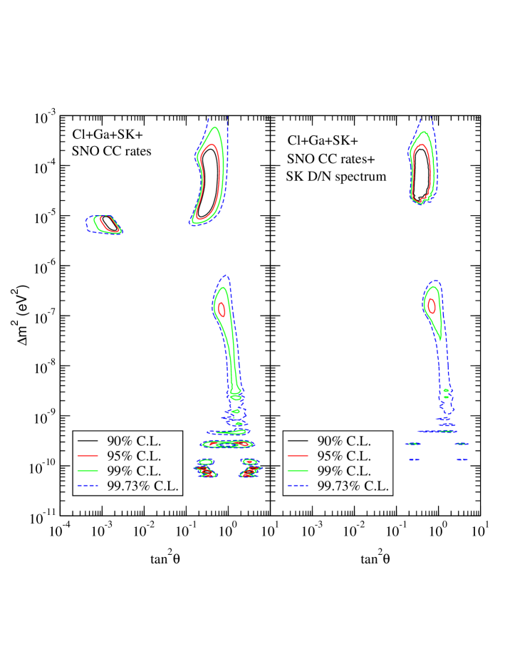
Figure 2: The 90%, 95%, 99% and 99.73% C.L. allowed areas from the analysis of the total rates (left panel) and global analysis of the rates and the 1258 day SK recoil electron spectrum at day and night (right panel), assuming MSW conversions to sequential neutrinos.

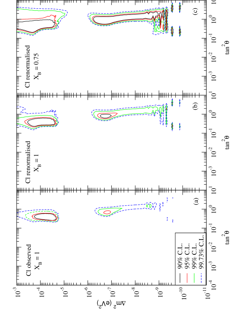
Figure 3: The 90, 95 and 99 and 99.73% C.L. allowed area from the global analysis of the total rates from Cl (observed and 20% renormalised), Ga,SK and SNO (CC) detectors and the 1258 days SK recoil electron spectrum at day and night, assuming MSW conversions to active neutrinos.

In fig. 2 we show the allowed regions in the $\Delta m^{2}-\tan^{2}\theta$ plane from the analysis of total rates and rate+spectrum. The significant change in the allowed regions after including the SNO results is the disappearance of the SMA region even at 99.73% C.L. ($3\sigma$) as a result of increased conflict between the total rates and SK spectrum data [28]. We see from fig. 2 that maximal mixing ($\tan^{2}\theta=1$) is not allowed in the LMA region but is allowed in the LOW region. In fig. 3 we show the allowed regions in $\Delta m^{2}-\tan^{2}\theta$ plane by
(i) using a Cl rate renormalised by 20% upwards in view of the fact that this is till an uncalibrated experiment
(ii) by using a ${}^{8}{B}$ flux normalisation factor of 0.75 in view of the large uncertainties associated with it due to the uncertainties in the ${{}^{7}{Be}}(p,\gamma){{}^{8}{B}}$ cross-section.
Both these cases gives an enlarged allowed region encompassing the maximal mixing solution for both LMA and LOW [29].

5.2.2 Energy independent solution

In Table 5 we give the results assuming an energy independent survival probability

$$P_{ee}=1-\frac{1}{2}\sin^{2}2\theta$$ (20)

	$X_{B}$	$\sin^{2}2\theta$ ($\tan^{2}\theta$)	$\chi^{2}_{\min}$	g.o.f
Chlorine	1.0	0.93(0.57)	46.06	23.58%
Observed	0.72	0.94(0.60)	44.86	27.54%
Chlorine	1.0	0.87(0.47)	41.19	41.83%
Renormalised	0.70	0.88(0.48)	38.63	48.66%

Table 5: The best-fit value of the parameter, the $\chi^{2}_{\min}$ and the g.o.f from a combined analysis of rate and spectrum with the energy independent solution [29].

This solution gives a better g.o.f to the global data as compared to the SMA solution.

5.2.3 Three Generation Neutrino Oscillation Parameters after SNO

We consider the picture $\Delta m^{2}_{21}=\Delta m^{2}_{\odot}$, $\Delta m^{2}_{31}=\Delta m^{2}_{CHOOZ},\simeq\Delta m^{2}_{atm}=\Delta m^{2}_{32}$
and the mixing matrix

$$U = \pmatrix{c_{13}c_{12}&s_{12}c_{13}&s_{13}\cr-s_{12}c_{23}-s_{23}s_{13}c_{12}&c_{23}c_{12}-s_{23}s_{13}s_{12}&s_{23}c_{13}\cr s_{23}s_{12}-s_{13}c_{23}c_{12}&-s_{23}c_{12}-s_{13}s_{12}c_{23}&c_{23}c_{13}\cr}$$ (21)

where we have neglected the CP violation phases. For $\Delta$m${}_{31}^{2}>>\Delta$m${}_{21}^{2}\approx$ the matter potential in sun , the $\nu_{3}$ state experiences almost no matter effect and MSW resonance can occur between $\nu_{2}$ and $\nu_{1}$ states. One can show the $\nu_{e}$ survival probability for this case to be

$$P_{ee}=c_{13}^{4}P_{ee}^{2gen}+s_{13}^{4}$$ (22)

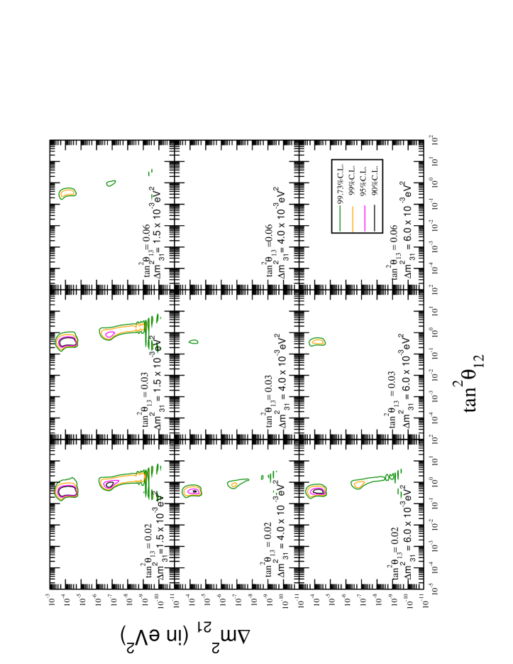
Figure 4: The allowed areas in $\tan^{2}\theta_{12}-\Delta m^{2}_{21}$ plane from solar+CHOOZ analysis for different fixed values of $\Delta m^{2}_{23}$ and $\tan^{2}\theta_{13}$.

where $P_{ee}^{2gen}$ is of the two generation form in the mixing angle $\theta_{12}$. We present in fig. 4 the allowed areas in the 1-2 plane at 90%, 95%, 99% and 99.73% confidence levels for different sets of combination of $\Delta m^{2}_{31}$ and $\tan^{2}\theta_{13}$, lying within their respective allowed range from atmospheric+CHOOZ and solar+CHOOZ analysis. Since CHOOZ data restricts $\tan^{2}\theta_{13}$ to very small values ($<0.075$) there is not much change in the allowed regions compared to the two-generation plots. In the three flavor scenario also there is no room for SMA MSW solution at the 3$\sigma$ level (99.73% C.L).The mixing matrix at the best-fit value of solar+CHOOZ analysis is [30]

$$U\simeq{\pmatrix{2\sqrt{\frac{2}{11}}&\sqrt{\frac{3}{11}}&0\cr-\sqrt{\frac{3}{22}}&\frac{2}{\sqrt{11}}&\frac{1}{\sqrt{2}}\cr\sqrt{\frac{3}{22}}&-\frac{2}{\sqrt{11}}&\frac{1}{\sqrt{2}}}}$$ (23)

Thus the best-fit mixing matrix is one where the neutrino pair with larger mass splitting is maximally mixed whereas the pair with splitting in the solar neutrino range has large but not maximal mixing.

6 Do we need a sterile neutrino?

The three neutrino oscillation phenomena mentioned above – namely the solar neutrino problem, the atmospheric neutrino anomaly and the $\nu_{\mu}-\nu_{e}$ oscillation observed by the LSND group – require three hierarchically different mass ranges,

$$\Delta m_{sun}^{2} \sim 5\times 10^{-5}\ eV^{2}\ , \sin^{2}2\theta\sim 0.8(LMA~{}~{}~{}MSW)$$

$$\Delta m_{Atm}^{2} \sim 3\times 10^{-3}\ eV^{2}, \ \sin^{2}2\theta\sim 1$$

$$\Delta m_{LSND}^{2} \sim 0.4-2\ eV^{2} \ \sin^{2}2\theta\sim 0.001-0.01$$

which cannot be accommodated in a three-generation picture. It has been widely realised that a remedy of this situation might be the introduction of a fourth neutrino. According to the LEP data there are three light active neutrino species. So the fourth neutrino has to be sterile. Introducing an additional sterile neutrino many schemes are possible. Detailed analysis shows that complete hierarchy of four neutrinos ($m_{1}<<m_{2}<<m_{3}<<m_{4}$) is not favoured by current data [31]. Mass patterns with three neutrino states closely degenerate in mass and the fourth one separated from these by the LSND gap (the 3+1 scheme) is also not preferred [32]. The 2+2 scheme in which two degenerate mass states are separated by the LSND gap is also disfavoured as it requires dominant oscillation to sterile neutrinos for either solar or atmospheric neutrinos. The still allowed scheme is the so called mixed 2+2 scheme in which the solar neutrino oscillation is due to $\nu_{e}$ going to a mixture of $\nu_{\tau}$ and $\nu_{s}$ and atmospheric neutrino problem can be explained by $\nu_{\mu}$ transition to a mixed state containing both $\nu_{\tau}$ and $\nu_{s}$ [33].

7 Goals for future experiments

In the context of the present picture it is worthwhile at this point to discuss what should be the major aims for the future experiments. These can be divided into two categories

7.1 Independent confirmation of the existing anomalies

Solar Neutrinos
The hints of neutrino oscillation coming from the earlier experiments is now established on a firm footing by the SK and SNO data. The main goal for the future experiments is discrimination between the LMA and LOW regions which are still allowed. Evidence in support of the LMA region is supposed to come from the KamLand experiment in Japan [34]. This is the first terrestrial experiment to probe the solar neutrino anomaly. It will look for oscillation by studying the flux and energy spectra of $\bar{\nu_{e}}$ produced by Japanese commercial nuclear reactors. The typical energy and length scales are $E_{\nu}\sim$ 3 GeV, L $\sim$ 3 $\times 10^{5}$ m , $\Delta m^{2}\sim 10^{-5}$ eV². Thus KamLand can probe the L/E dependence of the oscillations in the LMA region. It has started taking data in January 2002 and the results are expected to come this year.

Borexino is a 300 tons of liquid scintillator detector using trimethyle boroxine as a target [35]. Its main focus is the detection of 0.862 MeV solar ${}^{7}{Be}$ neutrinos which requires ultra low natural radioactive levels. A 4 tons prototype called counting test facility (CTF) has demonstrated extremely low radioactive level ($10^{-16}$g/g of U/th) can be achieved. SSM predicts $\sim$ 55/day in Borexino while SMA, LMA, LOW and VO solutions predict respectively $\sim$ 10-12/day, LMA $\sim$ 24/day, LOW $\sim$ 23/day, VAC $\sim$ 10-45/day with seasonal variations. Although LMA and LOW has almost the same number of events Borexino can distinguish between these two since the LOW region gives rise to a day-night asymmetry in Borexino due to earth regeneration
Atmospheric Neutrinos
Plans to increase the sensitivity of the accelerator neutrino oscillation experiments, by extending the baseline beyond the limits of the laboratory by sending intense neutrino beams towards a large and far away detector are in progress. These are the proposed long baseline experiments. These can have a sensitivity down to $\Delta{m}^{2}$ $\approx 10^{-3}$ eV² and using these one can cross-check the atmospheric neutrino results using neutrino beams of well known properties. K2K is the first Long baseline experiment to declare its data [36] and it reports a positive evidence of oscillation as we have heard from the previous speaker. The P-875 (MINOS) project plans to send a $\nu_{\mu}$ beam from FNAL to the Soudan mine [37] with a baseline of 730 km. It will have maximum sensitivity to $\nu-\mu-\nu_{\tau}$ and $\nu_{\mu}-\nu_{e}$ oscillations in the parameter space suggested by the SK atmospheric neutrino data. In Europe one proposed project is to send a beam from CERN to the ICARUS detector in the Gran Sasso underground laboratory in Italy with $L$ = 732 km [38] and explore $\nu_{\mu}-\nu_{\tau}$ and $\nu_{\mu}-\nu_{e}$ oscillations.

There is a proposal of a massive magnetized tracking calorimeter (MONOLITH) for detecting the atmospheric muon neutrinos and directly observing the $L/E$ pattern [39].
LSND
Independent confirmation of LSND results are expected to come from the Miniboone experiment at Fermilab which is scheduled to start collecting data soon [40].

7.2 Precise determination of the oscillation parameters

The SK and SNO data has provided the long awaited evidence in favour of neutrino oscillation. The future experiments are now geared towards determining the oscillation parameters accurately and determine the leptonic CKM matrix. Important role will be played by the long baseline experiments discussed earlier and by the proposed neutrino factories [41]. These will use muon storage rings to produce intense neutrino beams. A 20-30 GeV neutrino factory with $10^{19}$ muon decays/year provide what is known as an entry-level machine whereas a 50 GeV neutrino factory providing 10²⁰ muon decays/year is termed an high-performance machine. Below I list which parameters can be determined to what precision from these experiments.
Kamland experiment can tell us how close ($\pm$ few %) $\sin^{2}2\theta_{12}$ to 1 and also it is possible to determine of $|\Delta m^{2}_{21}|$ precisely (to within 10%) if LMA solution is the correct one. $\sin^{2}2\theta_{13}$ can be determined with a precision of $\sim$ 0.01 (long baseline experiments), $0.001$ ( entry level neutrino factory ), $\sim 10^{-4}$ ( high performance neutrino factory). $\sin^{2}2\theta_{23}$ can be determined to an accuracy of 10% (long baseline accelerator experiments and entry level neutrino factories) and in high performance neutrino factories this can be improved to $<5$%. $\Delta m^{2}_{23}$ can be determined by long baseline accelerator experiments and entry level neutrino factories to an accuracy of $\sim$ 10%. and in high performance neutrino factories it can be determined to within $<$ 1%. Sign of $\Delta m^{2}_{23}$ (normal or inverted hierarchy) can be determined from studying the matter effects on neutrino propagation in long baseline accelerator experiments and Neutrino Factories. CP violation in the lepton sector can be probed in neutrino factories, A new tritium beta decay experiment KATRIN is being planned to have a sensitivity limit of $\sim$ 0.3 eV [42]. This can provide the complimentary information on the absolute neutrino mass scale. Neutrino less double beta decay experiments are planned to have an increases sensitivity to $\langle{m_{ee}}\rangle$. These are CURORE ($\sim 0.1$ eV), MOON ($\sim 0.03$ eV), GENIUS ($\sim 0.002$ eV) [43].

8 Concluding Remarks

Last twenty years have seen a substantial progress in finding a definite answer to the question of neutrino mass and neutrino oscillation has emerged as a powerful probe to explore small neutrino masses. We now have two conclusive evidences in favour of neutrino flavour conversion coming from the
$\bullet$ The up/down asymmetry of the atmospheric muon neutrinos observed by SuperKamiokande signifies dominant $\nu_{\mu}-\nu_{\tau}$ conversion.
$\bullet$ Combination of SuperKamiokande and the SNO charged current (CC) data signals the presence of $\nu_{\mu}$/$\nu_{\tau}$ in the solar $\nu_{e}$ flux at more than 3$\sigma$ level.
$\bullet$ The most plausible and comprehensive explanation of both atmospheric and solar neutrino problem comes in terms of neutrino oscillation. The atmospheric neutrino anomaly indicates $\Delta m^{2}\sim 10^{-3}$ eV² and $\tan^{2}\theta\sim 1$. The solar neutrino data gives a best-fit $\Delta m^{2}\sim 5\times 10^{-5}$ eV² and $\tan^{2}\theta\sim 0.38$. Thus both atmospheric and solar neutrino problem indicate large mixing angles.
$\bullet$ The combined effect of SNO CC data and the SK recoil electron spectrum data disfavours SMA solution to the solar neutrino problem and no allowed region is obtained in this region at 3$\sigma$ level from the global analysis.
$\bullet$ A three generation analysis involving solar, atmospheric and CHOOZ data indicate a small value of $\tan^{2}\theta_{13}$ ($<0.075$) which is the common mixing angle connecting both solar and atmospheric sectors. Because of this the allowed regions in $\Delta m^{2}_{12}$ and $\theta_{12}$ for solar and $\Delta m^{2}_{23}$ and $\theta_{23}$ for atmospheric remain almost the same as in the two generation case.
$\bullet$ If the LSND data of positive evidence of neutrino oscillation is taken to be true then one requires the presence of a sterile neutrino. Of many models involving sterile neutrinos only the mixed 2+2 models are still consistent with the current data on solar and atmospheric neutrinos.
$\bullet$ Future experiments are planned to establish the oscillation solution by observing the actual oscillation pattern.
$\bullet$ With the conventional long baseline and neutrino factory experiments neutrino physics will enter the era of precision measurements.

Note Added: This talk was given in January 2002. The global analyses presented in the talk include the SNO CC data and the 1258 day SK spectrum data. Since then we have the 1496 day zenith angle spectrum data [23] and the SNO NC data [44, 45]. The main results are (i) The total flux measured with the NC reaction is consistent with the SSM value. (ii)Comparison of the SNO NC and the CC results establishes an active non-electron flavour component in the solar $\nu_{e}$ flux at more than 5$\sigma$ level.(iii)The probability of the LOW region decreases considerably as a combined effect of including the SNO NC data as well as the 1496 day SK spectrum data.

I thank the organizers of whepp-7 for inviting me to give this talk. I would like to acknowledge my collaborators A. Bandyopadhyay, S. Choubey, A.Joshipura, K. Kar, D.Majumder, D.P. Roy and A. Raychaudhuri.

References

- [1] A.I. Belesev et al., Preprint No. INR 862/94 (1994).
- [2] K. Assamagan et al., Preprint No.PSI-PR-94-19, (1994).
- [3] D. Buskulic et al., Phys. Lett. B349, 585 (1995).
- [4] H. V. Klapdor-Kleingrothaus et al, Euro. Phys. Journal, A12 (2001) 147; F. Feruglio, A. Strumia and F. Vissani, hep-ph/0201291.
- [5] L. Wolfenstein, Phys. Rev. D34, 969 (1986); S. P. Mikheyev and A. Yu. Smirnov, Sov. J. Nucl. Phys. 42, 913 (1985); Nuovo Cimento, 9C, 17 (1986).
- [6] C. Athanassopoulos et al., (The LSND Collaboration) Phys. Rev. Lett. 77, 3082 (1996); ibid. 81, 1774 (1998); A. Aguilar et al., (The LSND Collaboration) hep-ex/0104049.
- [7] Talk presented by The Karmen Collaboration (K Eitel for the Collaboration) in Neutrino 2000 held at Sudbury, Canada, Nucl. Phys. Proc. Suppl. 91, 191 (2001).
- [8] L. Borodovsky et al., Phys. Rev. Lett. 68, 274 (1992).
- [9] S. Choubey, P.hD. thesis, hep-ph/0110189.
- [10] T. K. Gaisser and J. S. O’Connell, Phys. Rev. D34, 822 (1986).
- [11] M. Honda, T. Kajita, S. Midorikawa, and K. Kasahara, Phys. Rev. D52, 4985 (1995).
- [12] Y. Fukuda et al., Phys. Lett. B335, 237 (1994).
- [13] D. Casper et al., Phys. Rev. Lett. 66, 2561 (1991); R. Becker-Szendy et al., Phys. Rev. D46, 3720 (1992).
- [14] Ch. Berger et al., Phys. Lett. B227, 489 (1989), Phys. Lett. B245, 305 (1990); Ch. Berger et al., Nucl. Instrum. Methods A261, 540 (1987).
- [15] M. Agiletta et al., Europhys. Lett. 8, 611 (1989).
- [16] M. Goodman et al., Nucl. Phys. (Proc. Suppl.) B38, 337 (1995).
- [17] T. Toshito, hep-ex/0105023.
- [18] For the details of the SuperKamiokande experiment and results see the article by Mark Vagins, Pramana-J. Phys. 60, 249 (2003).
- [19] J.N. Bahcall, S. Basu, M.P. Pinsonneault, Phys. Lett. B433, 1 (1998); Astrophys. J. 555, 990 (2001).
- [20] B.T. Cleveland et al. Astrophys. J 496, 505 (1998).
- [21] J.N. Abdurashitov et al., (The SAGE collaboration), Phys. Rev. C 60, 055801 (1999); W. Hampel et al., (The Gallex collaboration), Phys. Lett. B388, 384 (1996); Phys. Lett. bf B447, 127 (1999); ; M. Altmann et al., (The GNO collaboration),Phys. Lett. bf B492,16 (2000).
- [22] Y. Fukuda et al., (The Kamiokande collaboration), Phys. Rev. Lett. 77, 1683 (1996).
- [23] M. B. Smy, hep-ex/0202020.
- [24] The SNO Collaboration (Q.R. Ahmad et al.), Phys. Rev. Lett. 87, 071301 (2001)
- [25] Y. Fukuda et al., Phys. Rev. Lett. 86, 5651 (2001).
- [26] S.T. Petcov, Phys. Lett. B214, 139, (1988); ,200,373, (1988); S.T. Petcov and J. Rich, Phys. Lett. B426, (1989); G.L. Fogli, E. Lisi, D. Montanino, A. Palazzo , Phys. Rev. D62, 113004, (2000).
- [27] S. Choubey, S. Goswami, K. Kar, A.R. Antia, S.M. Chitre, Phys. Rev. D64, 113001 (2001).
- [28] G.L. Fogli, E. Lisi, D. Montanino and A. Palazzo, hep-ph/0106247; J.N. Bahcall, M.C. Gonzalez-Garcia and C. Penya-Garay, hep-ph/0106258; A. Bandyopadhyay, S. Choubey, S. Goswami and K. Kar, Phys. Lett. B519, 83 (2001).
- [29] S. Choubey, S. Goswami and D.P. Roy, Phys. Rev. D65, 073001 (2002).
- [30] A. Bandyopadhyay, S. Choubey, S. Goswami and K. Kar, Phys. Rev. D65, 073031 (2002).
- [31] S. M. Bilenky,,C. Giunti and W. Grimus, Euro. Phys. Journal C1 (1998)247; S. M. Bilenky et. al. Phys. Rev. D60 (1999) 073007.
- [32] . Maltoni, T. Schwetz and J. W. Valle, Phys. Lett. B 518 (2001) 252.
- [33] M. C. Gonzalez-Garcia, M. Maltoni and C. Pena-Garay, hep-ph/0108073.
- [34] S. A. Dazeley [KamLAND Collaboration], hep-ex/0205041.
- [35] . T. J. Beau, arXiv:hep-ex/0204035.
- [36] S.H. Ahn et al., (The K2K collaboration), Phys. Lett. B511, 178 (2001).
- [37] V. Paolone, Nucl. Phys. Proc. Suppl. 100 (2001) 197.
- [38] J. Rico [ICARUS Collaboration], hep-ex/0205028.
- [39] F. Terranova [MONOLITH Collaboration], Int. J. Mod. Phys. A 16S1B (2001) 736
- [40] E. A. Hawker, Int. J. Mod. Phys. A 16S1B (2001) 755.
- [41] V. D. Barger, S. Geer, R. Raja and K. Whisnant, Phys. Rev. D 62 (2000) 073002 and references therein.
- [42] Y. Farzan, O. L. Peres and A. Y. Smirnov, Nucl. Phys. B 612 (2001) 59.
- [43] E. Fiorini et al., Phys. Rep. 307 (1998) 309; H. Ejiri et. al. Phys. Rev. Lett. 85 (2000) 2917; GENIUS Collaboration (H. V. Klapdor-Kleingrothaus et al.), hep-ph/9910205.
- [44] The SNO Collaboration (Q.R. Ahmad et al.), (submitted to Phys. Rev. Lett.), nucl-ex/0204008.
- [45] The SNO Collaboration (Q.R. Ahmad et al.), (submitted to Phys. Rev. Lett.), nucl-ex/0204009.