Lepton Flavor Violation and Neutrino Mixings in a $3\times 2$ Seesaw Model

Abstract

We study the predictions for $BR(\mu\rightarrow e+\gamma)$ and $BR(\tau\rightarrow e,\mu+\gamma)$ in a class of recently proposed horizontal $SU(2)$ model that leads to a $3\times 2$ seesaw model for neutrino masses. We consider two such models and obtain the correct bi-large mixing pattern for neutrinos. In these models, the effective low energy theory below the $SU(2)_{H}$ scale is the MSSM. Assuming a supersymmetry breaking pattern as in the minimal SUGRA models, we find that consistent with present g-2, $b\rightarrow s+\gamma$ and WMAP dark matter constraints on the parameters of the model, the $BR(\mu\rightarrow e+\gamma)$ prediction is accessible to the proposed MEG experiment at PSI making this class of models testable in the near future.

I Introduction

Evidences for neutrino oscillations and hence for neutrino masses and mixings seem to be getting more and more solid. The results from solar and atmospheric neutrino experiments as well as those using terrestrial neutrinos as in the K2K and KAMLAND experiments which are responsible for this very important conclusion have together with CHOOZ and PALO-VERDE experiments clearly established the mixing pattern among different neutrino generations. It seems that two of the three neutrino mixings i.e. $\theta_{12}$ and $\theta_{23}$ are large and the third angle $\theta_{13}$ is smallreview . We will follow the literature and call this the bi-large mixing pattern.

This good news on the mixing front is however not shared by the masses i.e. our knowledge of the neutrino mass pattern is far from clear. At the moment three obvious possibilities i.e. (i) normal mass hierarchy, (ii) inverted mass hierarchy and (iii) degenerate mass pattern are equally viable. The challenge for future experiments is therefore twofold: to pin down the mass pattern more definitively and to improve measurements of the three angles to more precise values so that different theoretical models can be tested. For example it has been noted that if the present upper limit on the angle $\theta_{13}$ drops by one order of magnitude, a lot of very interesting models for neutrino masses will be ruled out. Of course more models being ruled out makes the direction of physics beyond the standard model that much more clear. It is therefore important to extract the predictions of the various models as far as possible to narrow the choices.

One of the very intriguing mass patterns for neutrinos is the inverted pattern, where the two heavier neutrinos are split by the solar mass difference $\Delta m^{2}_{\odot}$, whereas their absolute mass value is the square root of the atmospheric mass difference square i.e. $\Delta m^{2}_{A}$. In the extreme limit where $\Delta m^{2}_{\odot}=0$, this mass matrix admits an $L_{e}-L_{\mu}-L_{\tau}$ symmetry. If this pattern is confirmed by experiments, the existence of the $L_{e}-L_{\mu}-L_{\tau}$ symmetry could provide a clue to new local symmetries that operate at the higher scales where neutrino masses arise.

In two recent paperskuchi , it was shown that if there is a leptonic $SU(2)_{H}$ horizontal symmetryother acting both on the left as well as the right handed leptons of the standard model, then the theory must have two right handed neutrinos to cancel the global $SU(2)_{H}$ Witten anomaly. This provides a rationale for the existence of the right handed neutrino needed for implementing the seesaw mechanism. This leads to a $3\times 2$ seesaw formula for neutrino masses. The resulting neutrino mass matrix naturally leads to an inverted mass pattern for the light neutrinos after seesaw mechanismseesaw and in a certain areas of the parameter space gives rise to an approximate $L_{e}-L_{\mu}-L_{\tau}$ symmetryemutau of the neutrino mass matrix. Thus if the inverted mass pattern for neutrinos is confirmed by experiments, the $SU(2)_{H}$ models must be given very serious consideration.

As discussed in ref.kuchi , there are two possible patterns for the charged lepton mass matrix in these models and since the PMNS mixing matrix gets contributions both from the charged lepton as well as the neutrino sector, there will be two sets of predictions for the neutrino mixings. In this paper, we focus on them separately and study their physical implications, especially their predictions for lepton flavor violating branching ratios $BR(\mu\rightarrow e+\gamma)$ and $BR(\tau\rightarrow e,\mu+\gamma)$.

The key point is that below the horizontal symmetry scale, the theory is the minimal supersymmetric standard model (MSSM) and as is well knownlfv1 ; lfv2 ; lfv3 ; bdm , the presence of lepton mixings leads to mixings between sleptons via the renormalization group evolution even though at the GUT scale all slepton masses being equal forbid any such mixings. These in turn lead to lepton flavor violating decays such as $BR(\mu\rightarrow e+\gamma)$ and $BR(\tau\rightarrow e,\mu+\gamma)$ through one loop graphs involving the gauginos.

In order to arrive at our result, we first fix the model parameters such that they lead to observed neutrino mixings. We then find that for both the models referred to above, in most of the allowed parameter space for MSSM, the $BR(\mu\rightarrow e+\gamma)$ is around $10^{-12}$, which is within the range of the next generation of experimentspsi . The constraints on the supersymmetry parameter space come not only from the collider searches for supersymmetry and the LEP bound on Higgs boson mass but also from the Brookhaven g-2 results as well as the WMAP dark matter constraintswmap . The last constraint arises from the lightest neutralino $\chi^{0}_{1}$ as the dark matter candidate and using the recent WMAP results for the dark matter content of the universe i.e. $0.094<\Omega h^{2}<0.129$ (2$\sigma$). In deriving these results, some assumptions are needed for supersymmetry breaking parameters of the model. We use the mSUGRA choicesugra at the GUT scale to obtain the constraints i.e. universal mass for superpartners, common gaugino mass and $A$-terms being proportional to the Yukawa couplings. It is important that the GUT scale is higher than the seesaw scale to get sizable flavor mixing effects.

This paper is organized as follows: in sec. 2, we briefly review the salient features of the $SU(2)_{H}$ models and write down the $3\times 2$ seesaw formulae for the neutrino masses and mixings as well as the charged lepton mass matrices. We also present the exact neutrino mixing matrices in the limit of zero electron masses. In sec. 3, we present the numerical analysis of the neutrino mixings and masses and write down the choices of the model parameters that are phenomenologically acceptable. In sec. 4, we discuss the predictions for lepton flavor violating branching ratios in the model for these choices of parameters. In sec. 5, we conclude with a summary of the results.

II Models for lepton mixing

We consider extensions of the MSSM where the gauge group extended to $SU(3)_{c}\times SU(2)_{L}\times U(1)_{Y}\times SU(2)_{H}$ above the seesaw scale. Below the seesaw scale the model is MSSM so that the usual results for gauge coupling unification and electrweak symmetry breaking hold.

The basic motivation for considering these models is to find a symmetry rationale for the existence of right handed neutrino othet than the fact that it is needed to implement the seesaw mechanism. An elegant extension of the standard model that brings in the right handed neutrino automatically is to include the local B-L symmetry in the theory i.e. theories based on the gauge group $SU(2)_{L}\times U(1)_{I_{3R}}\times U(1)_{B-L}$ or $SU(2)_{L}\times SU(2)_{R}\times U(1)_{B-L}$ or the GUT group SO(10). Since our understanding of neutrino physics is not complete, it is important to explore other possibilities.

A different possibility is to look for horizontal (or family) symmetries that arise in the standard model in the limit of vanishing fermion masses. To see the possibilities, let us work with the extension of the standard model based on the gauge group $G_{STD}\times G_{H}$, where $G_{H}$ actos on the different generations. Three interesting possibilities that provide independent motivations for the existence of right handed neutrinos are: (i) $G_{H}=SU(3)_{q+\ell}$kribs ; (ii) $G_{H}=SU(2)_{q+\ell}$ kuchi and (iii) $G_{H}=SU(2)_{\ell}$kuchi with the obvious choice of fermion assignments. Here we will work with the case (iii) where we assume that the quark superfields transform under the $SU(2)_{H}$ group as singlets and leptons as doublets. In this case, it was noted in kuchi that while this model is free of local anomalies, absence of global Witten anomalieswitten implies that one must add two right handed neutrinos to the theory. Thus the existence of the right handed neutrinos are required for the consistency of the theory and not just to implement the seesaw mechanism. This is the model we want to study in detail in this paper.

The assignment of the leptons and Higgs superfields under the gauge group $SU(3)_{c}\times SU(2)_{L}\times U(1)_{Y}\times SU(2)_{H}$ is given as follows:

Table I

$\Psi\equiv(L_{e},L_{\mu})$	(1,2,-1,2)
$L_{\tau}$	(1,2,-1,1)
$E^{c}\equiv(\mu^{c},-e^{c})$	(1,1,-2, 2)
$\tau^{c}$	(1,1,-2, 1)
$N^{c}\equiv(\nu^{c}_{\mu},-\nu^{c}_{e})$	(1,1,0,2)
$\nu^{c}_{\tau}$	(1,1,0,1)
$\chi_{H}\equiv\left(\begin{array}[]{cc}\chi_{1}&\chi_{2}\\ \end{array}\right)$	(1, 1, 0, 2)
$\bar{\chi}_{H}\equiv\left(\begin{array}[]{cc}-\bar{\chi}_{2}&\bar{\chi}_{1}\\ \end{array}\right)$	(1,1,0,2)
$H_{u}$	(1,2,1,1)
$H_{d}$	(1,2,-1,1)
$\Delta_{H}$	(1,1,0,3)

Table caption: We display the quantum number of the matter and Higgs superfields of our model.

Here $L_{e,\mu,\tau}$ denote the left handed lepton doublet superfields. We arrange the Higgs potential in such a way that the $SU(2)_{H}$ symmetry is broken by $<\chi_{1}>=<\bar{\chi}_{2}>=v_{H1};<\chi_{2}>=<\bar{\chi}_{1}>=v_{H2}$ and $<\Delta_{H,3}>=v^{\prime}_{H}$, where $v_{H,i},v^{\prime}_{H}\gg v_{wk}$. The vevs for $\bar{\chi}$ are chosen so as to cancel the D-terms and leave supersymmetry unbroken below the scale $v_{H}$. Note that we have used the $SU(2)_{H}$ symmetry to align the $\Delta_{H}$ vev along the $I_{H,3}$ direction. At the weak scale, all the neutral components of the fields $H_{u}$ and $H_{d}$ acquire nonzero vev’s and break the standard model symmetry down to $SU(3)_{c}\times U(1)_{em}$. We denote these vev’s as follows: $<H^{0}_{u}>=\kappa_{0}$ and $<H^{0}_{d}>=\kappa_{0}cot\beta$; Clearly $\kappa_{0}$ has values in the 100 GeV range depending on the value of $tan\beta$.

Note that $<\Delta_{H}>\neq 0$ breaks the $SU(2)_{H}$ group down to the $U(1)_{L_{e}-L_{\mu}}$ group which is further broken down by the $\chi_{H}$ vevs. Since the renormalizable Yukawa interactions do not involve the $\chi_{H}$ field, this symmetry ($L_{e}-L_{\mu}$) is also reflected in the right handed neutrino mass matrix. This turns out to play a crucial role in leading to a bimaximal mixing pattern.

To discuss the detailed leptonic mixings, we now write down the Yukawa superpotential of the theory. The two models we discuss arise from the two ways the horizontal doublets couple to fermion superfields. In one case, we will allow only the $\chi_{H}$ field to couple to all fermions (to be called model I) and in the second case, we will allow the $\chi_{H}$ to couple to the right handed neutrino sector only and $\bar{\chi}_{H}$ to couple to the charged leptons only. This will be called model II.

II.1 Model I

The Yukawa superpotential for this model is given by:

$$W_{Y} = h_{0}(L_{e}H_{u}\nu^{c}_{e}+L_{\mu}H_{u}\nu^{c}_{\mu})+h_{1}L_{\tau}(\nu^{c}_{\mu}\chi_{2}+\nu^{c}_{e}\chi_{1})H_{u}/M-ifN^{cT}\tau_{2}{\bf\tau\cdot\Delta_{H}}N^{c}$$

$$\frac{h^{\prime}_{1}}{M}(L_{e}\chi_{2}-L_{\mu}\chi_{1})H_{d}\tau^{c}+\frac{h^{\prime}_{4}}{M}L_{\tau}H_{d}(\mu^{c}\chi_{2}+e^{c}\chi_{1})+{h^{\prime}_{3}}L_{\tau}H_{d}\tau^{c}+h^{\prime}_{2}(L_{e}e^{c}+L_{\mu}\mu^{c})H_{d}$$

This can be made natural by a choice of the discrete $Z_{2}$ symmetry under which $\bar{\chi_{H}}$ is odd and all other fields even, so that it does not couple to matter fields in the superpotential. $<\Delta^{0}_{H}>=v^{\prime}_{H}$ directly leads to the $L_{e}-L_{\mu}$ invariant $\nu_{eR}-\nu_{\mu R}$ mass matrix at the seesaw scale, as already noted. The $\chi_{H}$ vev contributes to this mass matrix only through nonrenormalizable operators and we assume those contributions to be negligible. We also do not include any term where $\Delta_{H}$ couples to light fields. Since the theory is supersymmetric, any term omitted from the superpotential will not be induced by loops due to the non-renormalization theorem. Similarly there will also be some small contributions from the $\nu_{\tau R}$ sector if we did not decouple it completely. We ignore these contributions in our analysis. Further, we define $\kappa_{1,2}=\frac{<\chi_{1,2}>\kappa_{0}}{M}\simeq 1-100$ GeV.

To study neutrino mixings in this model, let us write down the $5\times 5$ mass matrix for neutrinos:

$$M_{\nu_{L},\nu_{R}}~{}=~{}\left(\begin{array}[]{ccccc}0&0&0&h_{0}\kappa_{0}&0\\ 0&0&0&0&h_{0}\kappa_{0}\\ 0&0&0&h_{1}\kappa_{1}&h_{1}\kappa_{2}\\ h_{0}\kappa_{0}&0&h_{1}\kappa_{1}&0&fv^{\prime}_{H}\\ 0&h_{0}\kappa_{0}&h_{1}\kappa_{2}&fv^{\prime}_{H}&0\end{array}\right)$$ (7)

This is a $3\times 2$ seesaw matrixkuchi ; fram and after seesaw diagonalization, it leads to a $3\times 3$ light neutrino mass matrix as follows:

$${\cal M}_{\nu}~{}=~{}-M_{D}M^{-1}_{R}M^{T}_{D}$$ (8)

where $M_{D}~{}=~{}\left(\begin{array}[]{cc}h_{0}\kappa_{0}&0\\ 0&h_{0}\kappa_{0}\\ h_{1}\kappa_{1}&h_{1}\kappa_{2}\end{array}\right)$; $M^{-1}_{R}~{}=~{}\frac{1}{fv^{\prime}_{H}}\left(\begin{array}[]{cc}0&1\\ 1&0\end{array}\right)$. The resulting light Majorana neutrino mass matrix ${\cal M}_{\nu}$ is given by:

$${\cal M}_{\nu}~{}=~{}-\frac{1}{fv^{\prime}_{H}}\left(\begin{array}[]{ccc}0&(h_{0}\kappa_{0})^{2}&h_{0}h_{1}\kappa_{0}\kappa_{2}\\ (h_{0}\kappa_{0})^{2}&0&h_{0}h_{1}\kappa_{0}\kappa_{1}\\ h_{0}h_{1}\kappa_{0}\kappa_{2}&h_{0}h_{1}\kappa_{0}\kappa_{1}&2h^{2}_{1}\kappa_{1}\kappa_{2}\end{array}\right)$$ (12)

To get the physical neutrino mixings, we also need the charged lepton mass matrix defined by $\bar{\psi}_{L}{\cal M}_{\ell}\psi_{R}$. This is where the difference between the two models appear.

In model I, the charged lepton mass matrix is given by

$${\cal M}_{\ell}~{}=~{}cot\beta\left(\begin{array}[]{ccc}h^{\prime}_{2}\kappa_{0}&0&-h^{\prime}_{1}\kappa_{2}\\ 0&h^{\prime}_{2}\kappa_{0}&h^{\prime}_{1}\kappa_{1}\\ h^{\prime}_{4}\kappa_{1}&h^{\prime}_{4}\kappa_{2}&h^{\prime}_{3}\kappa_{0}\end{array}\right).$$ (16)

In order to study physical neutrino mixings, we must diagonalize the ${\cal M}_{\nu}$ and $M_{\ell}$ matrices. In ref.kuchi , we diagonalized the neutrino mass matrix analytically in the limit $m_{e}=0$. Let us discuss it for completeness. Since $h^{\prime}_{2}\kappa_{0}$ is proportional to the electron mass, we will ignore temporarily. Then, defining the matrices that diagonalize the charged lepton mass matrix as $D_{\ell}=U^{(L)}_{\ell}M_{\ell}U^{(R)\dagger}_{\ell}$, we get

$$U^{(L)}_{\ell}=\left(\begin{array}[]{ccc}s_{1}&c_{1}&0\\ c_{\beta}c_{1}&-c_{\beta}s_{1}&s_{\beta}\\ -s_{\beta}c_{1}&s_{\beta}s_{1}&c_{\beta}\end{array}\right)$$ (20)

where two angles $\theta_{1,2}$ are given by:

$$sin\theta_{1}\equiv s_{1}=\frac{\kappa_{1}}{\sqrt{\kappa_{1}^{2}+\kappa_{2}^{2}}}$$ (21)

$$sin\theta_{2}\equiv s_{2}=\frac{h_{0}\kappa_{0}}{\sqrt{h^{2}_{0}\kappa^{2}_{0}+h^{2}_{1}(\kappa^{2}_{1}+\kappa^{2}_{2})}}$$

and $tan2\beta\simeq 2\sqrt{\frac{h^{\prime}_{1}}{h^{\prime}_{4}}}\sqrt{m_{\mu}/m_{\tau}}$ and we have ignored terms of order $m_{e}/m_{\mu}$. Similarly the matrix that diagonalizes ${\cal M}_{\nu}$ is given by

$$U_{\nu}~{}=~{}\left(\begin{array}[]{ccc}c_{1}c^{\prime}-s_{1}s_{2}s^{\prime}&c_{1}s^{\prime}+s_{1}s_{2}c^{\prime}&c_{2}s_{1}\\ -s_{1}c^{\prime}-c_{1}s_{2}s^{\prime}&-s_{1}s^{\prime}+c_{1}s_{2}c^{\prime}&c_{2}c_{1}\\ -c_{2}s^{\prime}&c_{2}c^{\prime}&-s_{2}\end{array}\right)$$ (25)

where $s^{\prime}=sin\theta^{\prime}$ with $\theta^{\prime}$ given by $tan2\theta^{\prime}=\frac{2s_{2}(c^{2}_{1}-s^{2}_{1})}{(1+s^{2}_{2})2s_{1}c_{1}}$. The PMNS matrix that is measured in neutrino oscillation is given by $U^{(L)}_{\ell}U_{\nu}$ and has the form, in the limit of $m_{e}=0$:

$${\bf\Large U}_{PMNS}=\left(\begin{array}[]{ccc}s_{2}s^{\prime}&s_{2}c^{\prime}&c_{2}\\ -(c^{\prime}c_{\beta}+c_{2}s^{\prime}s_{\beta})&-(c_{\beta}s^{\prime}-s_{\beta}c_{2}c^{\prime})&-s_{2}s_{\beta}\\ (c^{\prime}s_{\beta}-c_{2}s^{\prime}c_{\beta})&(c_{2}c^{\prime}c_{\beta}+s^{\prime}s_{\beta})&s_{2}c_{\beta}\end{array}\right)$$ (29)

Using this, it was concluded in kuchi that there is an approximate relation between the neutrino parameters given by:

$$U^{2}_{e3}cos2\theta_{\odot}\simeq\frac{\Delta m^{2}_{\odot}}{2\Delta m^{2}_{A}}$$ (30)

It is clear from the above equation that for a given value of $\Delta m^{2}_{\odot}/\Delta m^{2}_{A}$, the smallest value of $U_{e3}$ will happen for the largest value of $sin^{2}2\theta_{\odot}$. In this paper first we numerically solve for the neutrino mixings and then proceed to calculate the lepton flavor violation effects for the allowed choices of the parameters of the model.

II.2 Model II

In this case, we impose a discrete symmetry under which the fields $(e^{c},\mu^{c},\tau^{c})$ and $\bar{\chi}_{H}$ are odd and all othee fields are even. The Yukawa superpotential invariant under this is:

$$W_{Y}~{}=~{}h_{0}(L_{e}H_{u}\nu^{c}_{e}+L_{\mu}H_{u}\nu^{c}_{\mu})+h_{1}L_{\tau}(\nu^{c}_{\mu}\chi_{2}+\nu^{c}_{e}\chi_{1})H_{u}/M-ifN^{cT}\tau_{2}{\bf\tau\cdot\Delta_{H}}N^{c}+$$ (31)

$$\frac{h^{\prime}_{1}}{M}(L_{e}\bar{\chi}_{1}+L_{\mu}\bar{\chi}_{2})H_{d}\tau^{c}+\frac{h^{\prime}_{4}}{M}L_{\tau}H_{d}(\mu^{c}\bar{\chi}_{1}-e^{c}\bar{\chi}_{2})+{h^{\prime}_{3}}L_{\tau}H_{d}\tau^{c}+h^{\prime}_{2}(L_{e}e^{c}+L_{\mu}\mu^{c})H_{d}$$

Note that the vev’s $<\bar{\chi}_{1,2}>=\kappa_{2,1}$ for the D-terms to cancel at the high scale. Substituting these vevs and the vev’s of $H_{u,d}$, we get exactly the same neutrino mass matrix as in model I i.e. Eq.12 but the charged lepton mass matrix becomes:

$${\cal M}_{\ell}~{}=~{}cot\beta\left(\begin{array}[]{ccc}h^{\prime}_{2}\kappa_{0}&0&h^{\prime}_{1}\kappa_{1}\\ 0&h^{\prime}_{2}\kappa_{0}&h^{\prime}_{1}\kappa_{2}\\ -h^{\prime}_{4}\kappa_{2}&h^{\prime}_{4}\kappa_{1}&h^{\prime}_{3}\kappa_{0}\end{array}\right).$$ (35)

The matrices that diagonalize this matrix are different from the first case (model I) and the $U^{(L)}_{\ell}$ in this case is given by:

$$U^{(L)}_{\ell}=\left(\begin{array}[]{ccc}c_{1}&-s_{1}&0\\ c_{\beta}s_{1}&c_{\beta}c_{1}&s_{\beta}\\ -s_{\beta}s_{1}&-s_{\beta}c_{1}&c_{\beta}\end{array}\right)$$ (39)

The ${\bf U}_{PMNS}$ in this case is given by

$${\bf\Large U}_{PMNS}=\left(\begin{array}[]{ccc}c^{\prime}&s^{\prime}&0\\ -s^{\prime}s_{2}c_{\beta}-c_{2}s^{\prime}s_{\beta}&s_{2}c^{\prime}c_{\beta}+c_{2}c^{\prime}s_{\beta}&c_{2}c_{\beta}-s_{2}s_{\beta}\\ (-s^{\prime}s_{2}s_{\beta}-c_{2}s^{\prime}c_{\beta})&(c_{2}c^{\prime}c_{\beta}-s_{2}c^{\prime}s_{\beta})&-s_{2}c_{\beta}-c_{2}s_{\beta}\end{array}\right)$$ (43)

Note that we have neglected corrections of order $\sqrt{m_{e}/m_{\mu}}$ and once they are turned on, we indeed have a nonzero $U_{e3}$ and small. We will discuss the detailed numerical predictions in the next section.

III Neutrino mass fit

III.1 MODEL I

The expressions for the Dirac neutrino matrix and the charged lepton matrix are given in the previous section. We will use those expressions in order to derive the light neutrino masses and the mixing angles numerically. That will fix the model parameters that will go into the renormalization group evolution of the slepton masses. We will generate the fit for different values of $\tan\beta$ and model parameters. For example, at $\tan\beta=30$, the charged lepton mass matrix is given by (at the scale where the horizontal symmetry gets broken) :

$${\cal M}_{\ell} = \left(\matrix{7.5\times 10^{-3}&0&-1.135\cr 0&7.5\times 10^{-3}&0.247\cr 2.14\times 10^{-2}&0.0984&0.85}\right).$$ (44)

This matrix needs $h_{1}^{\prime}=1.135\times 10^{-1}$, $h_{2}^{\prime}=1.29\times 10^{-3}$, $h_{3}^{\prime}=1.466\times 10^{-1}$ and $h_{4}^{\prime}=9.8\times 10^{-3}$ with $\kappa_{2}=10$ and ${\kappa_{2}\over\kappa_{1}}=4.588$. We get the correct values of charged lepton masses at the weak scale from the above matrix. We use the MSSM RGEs between the horizontal scale and the weak scale. Using the same $\kappa$s, $h_{0}=9.2\times 10^{-2}$ and $h_{1}=-2.92\times 10^{-1}$, we find the light neutrino mass matrix (in eV):

$${\cal M}_{\nu} = \left(\matrix{0&5.15\times 10^{-2}&-9.3\times 10^{-3}\cr 5.15\times 10^{-2}&0&-2.04\times 10^{-3}\cr-9.3\times 10^{-3}&2.04\times 10^{-3}&7.4\times 10^{-4}}\right).$$ (45)

The PMNS matrix and neutrino eigenvalues at the weak scale are :

$${\bf\Large U}_{PMNS} = \left(\matrix{0.806&0.58&-0.109\cr-0.27&0.527&0.805\cr 0.526&-0.619&0.582}\right).$$ (46)

$$(m_{1},~{}m_{2},~{}m_{3})=(5.276\times 10^{-2},\,5.202\times 10^{-2},\,0)~{}{\rm eV}~{}.$$ (47)

From the above fit, we find $\sin^{2}2\theta_{\odot}=0.87$, $\Delta m^{2}_{\odot}=7.7\times 10^{-5}$ eV² and $\sin^{2}2\theta_{A}=0.88$, $\Delta m^{2}_{A}=2.7\times 10^{-3}$ eV² which are well allowed by the experimental results.

The above fit is obtained for a particular value of $\kappa_{2}\over\kappa_{1}$. We can change that value and the Yukawa couplings $h$s and $h^{\prime}$s and still can obtain very good fits. In fig.1 we show the model points which are within the experimental limits of $\sin^{2}2\theta_{\odot}$ and $\sin^{2}2\theta_{A}$. We find many model points which satisfy the allowed ranges. In Fig.2, we show the $|U_{e3}|$ as a function of $\sin^{2}2\theta_{\odot}$ for the model points which satisfy the experimental limit on $\sin^{2}2\theta_{A}$. The range of $U_{e3}$ is 0.07-0.13 in this model and is allowed by the current experimental upper bound 0.22fl . In fact, it is expected that the planned long base line experiments including MINOS have the ability to probe this range in the next few years.

The scale of the horizontal symmetry breaking is assumed to be $3\times 10^{13}$ and the magnitude of the Majorana coupling is $f\sim 1.6\times 10^{-1}$. The fit does not change if we move the scale up or down.

The fit for $\tan\beta=$10 and 40 look similar. The charged lepton mass matrices for these two $\tan\beta$ are given below.
For $\tan\beta=40$ we have:

$${\cal M}_{\ell} = \left(\matrix{8.2\times 10^{-3}&0&-1.30\cr 0&8.2\times 10^{-3}&2.83\times 10^{-1}\cr 2.33\times 10^{-2}&1.07\times 10^{-1}&9.5\times 10^{-1}}\right).$$ (48)

We keep the light neutrino matrices unchanged and we find $\sin^{2}2\theta_{\odot}=0.88$, $\Delta m^{2}_{\odot}=7.7\times 10^{-5}$ eV² and $\sin^{2}2\theta_{A}=0.87$, $\Delta m^{2}_{A}=2.7\times 10^{-3}$ eV².
For $\tan\beta=10$ we have:

$${\cal M}_{\ell} = \left(\matrix{6.8\times 10^{-3}&0&-9.9\times 10^{-1}\cr 0&6.8\times 10^{-3}&2.15\times 10^{-1}\cr 2.088\times 10^{-2}&9.58\times 10^{-2}&8.0\times 10^{-1}}\right).$$ (49)

We keep the light neutrino matrices unchanged and we find $\sin^{2}2\theta_{\odot}=0.88$, $\Delta m^{2}_{\odot}=7.7\times 10^{-5}$ eV² and $\sin^{2}2\theta_{A}=0.92$, $\Delta m^{2}_{A}=2.7\times 10^{-3}$ eV².

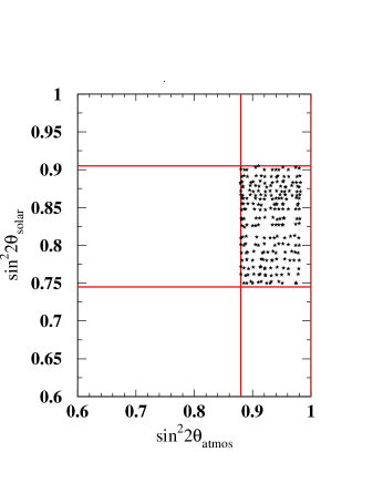
Figure 1: $sin^{2}2\theta_{\odot}$ vs $sin^{2}2\theta_{\rm atmos}$. The stars show the model points. The horizontal and vertical solid lines show the current experimental limits.

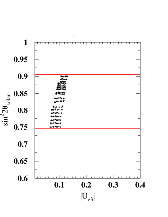
Figure 2: $sin^{2}2\theta_{\odot}$ vs $|U_{e3}|$. The stars show the model points. The horizontal solid lines show the current experimental limits.

III.2 MODEL II

In this model, the Dirac neutrino matrix is similar to what we have in the previous model. The charged lepton matrix is the transpose of that in the other case. We can again obtain the neutrino fit for different values of $\tan\beta$. For example, at $\tan\beta=30$, The charged lepton mass matrix is given by (at the scale where the horizontal symmetry breaks down):

$${\cal M}_{\ell} = \left(\matrix{8.28\times 10^{-2}&0&5.0\times 10^{-5}\cr 0&8.28\times 10^{-2}&4.0\times 10^{-3}\cr-1.44&0.018&6.9\times 10^{-3}}\right).$$ (50)

This matrix requires $h_{2}^{\prime}$=0.0143, $h_{3}^{\prime}=1.2\times 10^{-3}$, $h_{1}^{\prime}=1.00\times 10^{-4}$, $h_{4}^{\prime}=3.6\times 10^{-2}$ for $\kappa_{2}=40$ and ${\kappa_{2}\over\kappa_{1}}=0.5$. The charged lepton mass matrix produces the correct values of charged lepton masses at the weak scale after using the RGEs. Using the same $\kappa$’s, $h_{0}=7.67\times 10^{-2}$ and $h_{1}=3.07\times 10^{-1}$ we find the light neutrino mass matrix:

$${\cal M}_{\nu} = \left(\matrix{0&3.55\times 10^{-2}&3.27\times 10^{-2}\cr 3.55\times 10^{-2}&0&4.09\times 10^{-4}\cr 3.27\times 10^{-2}&4.09\times 10^{-4}&7.5\times 10^{-4}}\right).$$ (51)

The PMNS matrix and neutrino eigenvalues are :

$${\Large\bf U}_{PMNS} = \left(\matrix{-0.724&0.68&-0.042\cr 0.527&0.513&-0.677\cr-0.44&-0.512&-0.734}\right).$$ (52)

$$(m_{1},~{}m_{2},~{}m_{3})=(4.87\times 10^{-2},\,4.79\times 10^{-2},\,0)~{}{\rm eV}~{}.$$ (53)

The solar angle prediction i.e. $sin^{2}2\theta_{\odot}=0.95$ for this model is on the higher side and therefore as the experimental error on $\theta_{12}$ narrows, this model will be tested. The atmospheric mixing angle $sin^{2}2\theta_{A}$ is 0.98 and is well allowed by the experimental results. The prediction for $U_{e3}=-0.042$ and it will also be probed in the near future.

In the following, the scale of horizontal symmetry breaking our calculations is assumed to be $3\times 10^{13}$ and the magnitude of the Majorana coupling is $f\sim 1.6\times 10^{-1}$.

IV Lepton Flavor Violation

It is well known that in the standard model where neutrino masses vanish, there is no lepton flavor violation. Once the neutrinos have masses as well as mixings, there are small amounts of lepton flavor violation leading to processes such as $\ell_{j}\rightarrow\ell_{i}+\gamma$ with $i\neq j$. However, if only a Dirac mass( by adding a right handed neutrino) or a Majorana mass (by adding a Higgs triplet) of the neutrino are added to the standard model, then lepton flavor violating processes which always arise at one loop or higher loop level in gauge theories have branching ratios proportional to $\left(\frac{m^{2}_{\nu}}{m^{2}_{W}}\right)^{2}$ and are therefore very tiny. In models with supersymmetry however, the situation can change drastically. In the presence of neutrino masses, the superpartners of leptons could in general mix and the LFV branching ratio in that case becomes of order$\left(\frac{m^{2}_{\tilde{\ell}}}{m^{2}_{W}}\right)^{2}$ where $m_{\tilde{\ell}}$ is a typical mass of the slepton and since the slepton masses are expected to be of order of the weak scale, the LFV branching ratios in general can be quite large. The actual magnitude however depends on the specific model for neutrino masses as well as on the pattern of supersymmetry breaking. If we assume the neutrino masses to arise from the seesaw mechanism, then depending on how the seesaw mechanism is implemented in a theory, the predictions for LFV can be different.

Similarly, the nature of supersymmetry breaking is also important since in the supersymmetric limit the radiative flavor changing decays vanish. To illustrate this point, let us consider a simple seesaw model where the susy breaking slepton masses are universal at the seesaw scale and the SUSY breaking $A$ terms are proportional to Yukawa couplings as in the minimal SUGRA models. We can go to a basis where the charged lepton Yukawa couplings are diagonal. This simply rotates the neutrino mass matrix and keeps all other terms in the Lagrangian flavor In such a theory, just below the seesaw scale, flavor mixing is present only in the neutrino masses from the seesaw formula. As we extrapolate the slepton masses down to the seesaw scale, they remain diagonal since the charged lepton Yukawa coupling is diagonal. The only source of lepton flavor violation is then in the neutrino masses. Therefore, in this case $BR(\mu\rightarrow e+\gamma)\propto\left(\frac{m^{2}_{\nu}}{m^{2}_{W}}\right)^{2}$ and is therefore negligible. To obtain a significant LFV effect therefore, one must assume that the universality of slepton masses and the proportionality of the $A$ terms must hold much above the seesaw scale. Fortunately, this is what is generally assumed in minimal SUGRA models anyway. Thus no observable LFV effect would simply be a manifestation of the fact that it is the seesaw scale where universality of slepton masses holds e.g. in models like gauge mediated supersymmetry breaking. In this paper, we will assume that the universality of scalar masses holds at a scale higher than the seesaw scale.

Turning to our case, since we only have an SU(2) horizontal symmetry, we can dispense with any assumption regarding universality and allow for the most general SUSY breaking pattern consistent with the $SU(2)_{H}$ symmetry. For definiteness, we will assume universality of scalar masses at a higher scale (e.g. the GUT scale) and use RGE effects of the lepton Yukawa couplings to get the slapton masses and the $A$ terms at the $v_{H}$ scale. This is a non-universal profile at the seesaw scale and leads to $m^{2}_{i}$ as a function of the Yukawa couplings. If we then rotate i.e. $m^{2}_{\tilde{e}}=m^{2}_{\tilde{\mu}}=m^{2}\simeq m^{2}_{0}+\frac{(6+2a^{2})(h^{2}_{0}+h^{{}^{\prime}2}_{2})m^{2}_{0}}{16\pi^{2}}\ell n\frac{M_{U}}{v_{H}}$ and $m^{2}_{\tilde{\tau}}=m^{2}_{0}+\frac{(6+2a^{2})(h^{{}^{\prime}2}_{3})m^{2}_{0}}{16\pi^{2}}\ell n\frac{M_{U}}{v_{H}}$. If we now rotate the charged lepton Yukawas just below the horizontal symmetry scale to go to a diagonal basis for charged lepton Yukawa couplings, we will generate slepton flavor mixings such as $m^{2}_{LL,13}$ and $m^{2}_{LL,23}$. A combination of these two terms at the weak scale will give rise to a nonvanishing branching ratio for $\mu\rightarrow e+\gamma$ and $\tau\rightarrow e,\mu+\gamma$. If we focus the slepton masses alone, we roughly get

$$B(\mu\rightarrow e+\gamma)\propto\frac{\alpha_{em}\alpha^{2}_{1}\delta^{2}(U_{e3}U_{\mu 3})^{2}}{G^{2}_{F}m^{4}_{0}}$$ (54)

One can also in a similar manner estimate the contribution of the $A$ terms. In fact it turns out that it is the $A$-term slepton mixings that make the dominant contribution to the LFV branching ratios in our model.

To proceed with the calculations for LFV processes in our case, we will use mSUGRA models which has five parameters at the GUT scale i.e. $m_{0}$, $m_{1/2}$, $A_{0}$, $\tan\beta$ and $\mu$sugra . We will assume that at the GUT scale all scalar masses have the common value $m_{0}$ as noted in the previous section; gauginos have the common mass $m_{1/2}$; the trilinear SUSY breaking terms are proportional to the Yukawa couplings and the rest of the theory is defined by the the superpotentials in section II. First note that the renormalization group evolution (RGE) is caused only by dimension four terms in the Lagrangian. The charged lepton Yukawa matrix responsible for the RGE from the GUT scale to the weak scale is diagonal since the only dimension four Yukawa couplings are $h^{\prime}_{2,3}$. Similarly, the dimension 4 Dirac neutrino couplings are also flavor diagonal with the Yukawa coupling $h_{0}$. Thus as we run down from the GUT scale to the horizontal symmetry breaking scale $v_{H}$, the slepton masses remain horizontal; The $A$ terms get modified.

The RGE from the $v_{H}$ scale down to the weak scale is the MSSM RGE. We generate the off diagonal elements of the charged lepton Yukawa matrix at the horizontal scale from the nonrenormalizable operators and Dirac neutrino matrix becomes a $3\times 2$ matrix. The off diagonal elements of the charged lepton mass matrix induce the flavor violating terms in the $m_{LL}^{2}$, $m_{LR}^{2}$ and $m_{RR}^{2}$ mass matrices via the RGEs from the horizontal scale down to the weak scale. For example, $E_{A_{12}}$ term (which contributes to $m_{LR}^{2}$) gets generated via terms $E_{A}U_{l}^{{\dagger}}U_{l}$, $U_{l}U_{l}^{{\dagger}}E_{A}$ pieces in the RGE (${dE_{A}\over{dt}}$$\propto{1\over{16\pi^{2}}}(4E_{A}U_{l}^{{\dagger}}U_{l}+5U_{l}U_{l}^{{\dagger}}E_{A})$, where $U_{l}$ is the $3\times 3$ matrix for the Dirac Yukawa coupling). We have $U_{13,31}$ and $U_{32,23}$ terms in both models. These terms generate large BR($\mu\rightarrow e+\gamma$).

The calculation of BR($\mu\rightarrow e+\gamma$)involves both neutralino and chargino diagram contribution. In some parameter space one type dominates and the other type dominates in some other. Before we discuss the BRs. of the lepton flavor violating decay modes, we need to discuss the supersymmetric parameter space.

IV.1 Supersymmetry parameter space

The mSUGRA parameter space is constrained by the experimental lower limit on $m_{h}$ and measurements of $b\rightarrow s\gamma$ and recent results on dark matter relic densitywmap . For low $\tan\beta$, the parameter space has lower bound on $m_{1/2}$ from the light Higgs mass bound of $m_{h}\geq 114$ GeV. For larger $\tan\beta$ the lower bound on $m_{1/2}$ is produced by the CLEO constraint on the BR($b\rightarrow s\gamma$). The recent WMAP results have led to stronger constraints on dark matter density which in turn reduces the allowed parameter space of MSSM mostly to the co-annihilation region for $m_{0},\,m_{1/2}\leq 1000$ GeV. As is well known, co-annihilation requires some other superpartner to have mass close to the lightest neutralino. In the mSUGRA model co-annihilation happens between the lightest slepton and the lightest neutralinocoan . One can see this analytically for low and intermediate $\tan\beta$ for mSUGRA where the RGE can be solved analytically b35 . At the electroweak scale one has for the average slepton masses

$$\tilde{m}_{e_{R}}^{2}=m_{0}^{2}+(6/5)f_{1}m_{1/2}^{2}-\sin^{2}\theta_{W}M_{W}^{2}\cos(2\beta)$$ (55)

$$m_{\tilde{\chi}_{1}^{0}}=(\alpha_{1}/\alpha_{G})m_{1/2}$$ (56)

where $f_{i}=[1-(1+\beta_{i}t)^{-2}]/\beta_{i}$, $t=\ln(M_{G}/M_{Z})^{2}$ and $\beta_{1}$ is the $U(1)$ $\beta$ function. Numerically this gives for e.g. $\tan\beta=$ 5

$$\tilde{m}_{\tilde{e}_{R}}^{2} = m_{0}^{2}\,+\,0.15m_{1/2}^{2}\,+(37\,{\rm GeV})^{2}$$

$$m_{\tilde{\chi}_{1}^{0}}^{2} = 0.16m_{1/2}^{2}$$ (57)

Thus for $m_{0}=$ 0, the $\tilde{e}_{R}$ becomes degenerate with the $\tilde{\chi}_{1}^{0}$ at $m_{1/2}=370$ GeV, i.e. coannihilation effects begin at $m_{1/2}\stackrel{{\scriptstyle\sim}}{{=}}(350-400)$ GeV. For larger $m_{1/2}$, the near degeneracy is maintained by increasing $m_{0}$, and there is a corridor in the $m_{0}-m_{1/2}$ plane allowing for an adequate relic density. For larger $\tan\beta$, the stau is the lightest slepton and its mass is close to the neutralino mass for a large region of parameter space.

The previous relic density bound $0.07<\Omega h^{2}<0.21$ reduced the parameter space mostly into coannihilation bands. The most recent WMAP result $0.094<\Omega h^{2}<0.129$ has narrowed the co-annihilation regions furtherwmap2 .

Further constraints on the parameter space arise from the present muon g-2 resultsads , if we take the deviation from the standard model value as an upper limit on the supersymmetric contribution to g-2. For instance, for $\tan\beta$=10, we get $m_{1/2}<430$ GeV. Since the Higgs mass implements a lower bound $m_{1/2}\geq$300 GeV, we do not have much parameter space left for this value of $\tan\beta$. However, for $\tan\beta$=30 and 40, the upper bounds are $m_{1/2}<720$ and 790 GeV respectively from the g-2 of muon data and thus the allowed parameter space becomes bigger. We will therefore restrict ourselves to larger values of $\tan\beta$ for the discussions of flavor violation BRs.

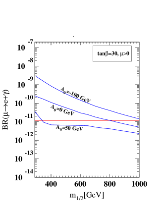
Figure 3: BR[$\mu\rightarrow e+\gamma$] as a function of $m_{1/2}$ for different values of $A_{0}$ for model I.

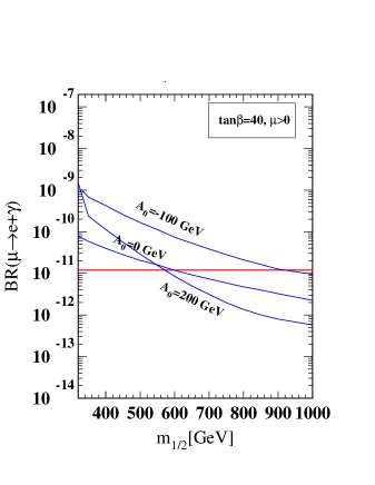
Figure 4: BR[$\mu\rightarrow e+\gamma$] as afunction of $m_{1/2}$ for different values of $A_{0}$ for model I.

In Figs.3 and 4, we show the BR($\mu\rightarrow e+\gamma$) for $\tan\beta$=30 and 40 for different values of $A_{0}$ in model I. We tune $m_{0}$ such so that $\Omega h^{2}$ constraint is satisfied. This mostly happens where the light stau mass is very close to the lightest neutralino mass. For example, for $m_{1/2}=400$ GeV, $m_{0}\sim$ 208-215 GeV satisfies the $\Omega h^{2}$ constraint for $\tan\beta=40$ and $A_{0}=0$. The BR remains almost unchanged over the small range of $m_{0}$. The parameter space shown in the figures are allowed by the BR$[b\rightarrow s\gamma]$ constraint. From these figures, we find that as $m_{1/2}$ increases BR decreases. In the figures, the dependence of the BR on $A_{0}$ is also shown. The relative sizes of the chargino and neutralino diagram contributions change with $A_{0}$. The BR, in most of the parameter space, is around $10^{-12}$. Choosing a smaller $\kappa_{2}\over\kappa_{1}$ ratio dcreases the BR ratio further. But this ratio has a lower bound from the fit to the solar mixing angle. The lowest possible BR is a factor of 2 smaller than what is shown in the figure. The BR also can be reduced by a factor of 4 if we increase the seesaw scale from $3\times 10^{13}$ to $10^{15}$

Turning to the BR($\tau\rightarrow\mu(e)+\gamma$), it is at least 3 order magnitude below the current experimental result in the parameter space allowed by the BR($\mu\rightarrow e+\gamma$).

In Figs 5 and 6, we show the BRs. for $\mu\rightarrow e+\gamma$ for $\tan\beta$=30 and 40 for $A_{0}$ =0 and $A_{0}=200$ GeV in model II. The $m_{0}$ is chosen such so that $\Omega h^{2}$ constraint is satisfied. The $\tau\rightarrow\mu(e)+\gamma$ BR is at least 3-4 order magnitude below the current experimental limits.

Furthermore, the parameter space where the BR($\mu\rightarrow e\gamma$) is larger, the other observables e.g. BR($B_{s}\rightarrow\mu\mu$) can be observed in the current RUN at the Tevatron. Similarly, for these values, $\sigma_{\tilde{\chi}^{0}_{1}-p}$ are also large adkt and can therefore be observable in planned dark matter experiments. Thus, once the parameter space is narrowed from these different measurements, this model can be deciphered by the $\mu\rightarrow e+\gamma$ experiment.

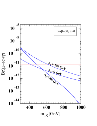
Figure 5: BR[$\mu\rightarrow e+\gamma$] as afunction of $m_{1/2}$ for different values of $A_{0}$ for model II.

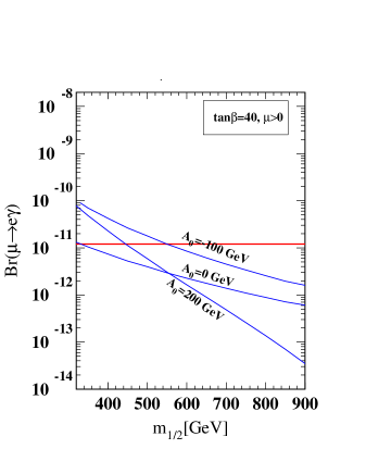
Figure 6: BR[$\mu\rightarrow e+\gamma$] as afunction of $m_{1/2}$ for different values of $A_{0}$ for model II.

V Conclusion

In summary, we have analysed two models with local SU(2) horizontal symmetry that lead naturally to bi-large mixing pattern for neutrinos. We determined the parameters of these models from the detailed numerical fit to the neutrino masses and the mixing angles. Using these models we then obtained predictions for lepton flavor violating decays BR[$\mu\rightarrow e+\gamma$] in mSUGRA framework. The parmeter space, we consider, is constrained by the following experimental constraints: BR[$b\rightarrow s\gamma$], Higgs mass and the recent relic density results from WMAP and the Brookheven g-2 experiment. We find that, in both models, the branching ratio is large in a large region of parameter space and is in the range accessible to the current round of searches for this process. This parameter space can simultaneously be explored at Tevatron, LHC and the upcoming of dark matter detectors.

The work of R. N. M. is supported by the National Science Foundation Grant No. PHY-0099544 and that of B. D. by the Natural Sciences and Engineering Research Council of Canada.

References

- (1) For recent reviews, see S. Bilenky, C. Giunti, J. Grifols and E. Masso, hep-ph/0211462 (Phys. Rep., to appear); S. Pakvasa and J. W. F. Valle, hep-ph/0301061.
- (2) R. Kuchimanchi and R. N. Mohapatra, Phys. Rev. D 66, 051301 (2002); Phys. Lett. B 552, 198 (2003).
- (3) D. S. Shaw and R. R. Volkas, Phys. Rev. D47, 241 (1993); R. Barbieri, L. Hall and A. Romanino, Phys. Lett. B401, 47 (1999); K. S. Babu and R. N. Mohapatra, Phys. Rev. Lett. 83, 2522 (1999); T. Blazek, S. Raby and K. Tobe, Phys. Rev. D62, 055001 (2000); S. Raby, hep-ph/0302027; N. Maekawa, hep-ph/0212141.
- (4) M. Gell-Mann, P. Rammond and R. Slansky, in Supergravity, eds. D. Freedman et al. (North-Holland, Amsterdam, 1980); T. Yanagida, in proc. KEK workshop, 1979 (unpublished); R.N. Mohapatra and G. Senjanović, Phys. Rev. Lett. 44, 912 (1980); S. L. Glashow, Cargese lectures, (1979).
- (5) R. Barbieri, L. Hall, D. Smith, A. Strumia and N. Weiner, hep-ph/9807235; A. Joshipura and S. Rindani, Eur.Phys.J. C14, 85 (2000); R. N. Mohapatra, A. Perez-Lorenzana, C. A. de S. Pires, Phys. Lett. B474, 355 (2000); T. Kitabayashi and M. Yasue, Phys. Rev. D 63, 095002 (2001); Phys. Lett. B 508, 85 (2001); hep-ph/0110303; L. Lavoura, Phys. Rev. D 62, 093011 (2000); W. Grimus and L. Lavoura, Phys. Rev. D 62, 093012 (2000); J. High Energy Phys. 09, 007 (2000); J. High Energy Phys. 07, 045 (2001); R. N. Mohapatra, hep-ph/ 0107274; Phys. Rev. D 64, 091301 (2001); K. S. Babu and R. N. Mohapatra, Phys. Lett. B 532, 77 (2002); H. S. Goh, R. N. Mohapatra and S.-P. Ng, hep-ph/0205131; Phys. Lett. B 542, 116 (2002); Duane A. Dicus, Hong-Jian He, John N. Ng, Phys. Lett. B 536, 83 (2002); Q. Shafi and Z. Tavartkiladze, Phys. Lett. B 482, 1451 (2000); Mass matrices with symmetry were discussed in S. Petcov, Phys. Lett. B 110 , 245 (1982).
- (6) F. Borzumati and A. Masiero, Phys. Rev. Lett. 57, 961 (1986); L. Hall, V. Kostelecky and S. Raby, Nucl. Phys. B267, 415, (1986).
- (7) J. Hisano, T. Moroi, K. Tobe, M. Yamaguchi and T. Yanagida, Phys. Lett. B357, 579 (1995); J. Hisano, T. Moroi, K. Tobe and M. Yamaguchi, Phys. Rev. D53, 2442 (1996).
- (8) S. F. King and M. Oliveira, Phys. Rev. D60, 035003 (1999); J. Hisano and D. Nomura, Phys. Rev. D59, 116005 (1999); K. S. Babu, B. Dutta and R. N. Mohapatra, Phys. Lett. B458, 93 (1999); W. Buchmuller, D. Delepine and F. Vissani Phys. Lett. B459, 171 (1999); J. Ellis, M. Gomez, G. Leontaris, S. Lola and D. Nanopoulos, Eur. Phys. J. C14, 319 (2000); T. Blazek and S. King, Phys. Lett. B518, 109 (2001); S. Lavgnac, I. Masina and C. Savoy, Phys. Lett. B520, 269 (2001); Nucl. Phys. B633, 139 (2002); J. Casas and A. Ibarra, Nucl. Phys. B618, 171 (2001); R. Gonzalez Felipe and F. Joaquim, JHEP 0109, 015 (2001); J. Sato, K. Tobe and T. Yanagida, Phys. Lett. B498, 189 (2001); X. J. Bi, Y. B. Dai and X. Y. Qi, Phys. Rev. D63, 096008 (2001), Phys. Rev. D66, 076006 (2002); G. Cvetic, C. Dib, C.S. Kim and J.D. Kim, Phys. Rev. D66, 034008 (2002); J. Ellis, J. Hisano, S. Lola and M. Raidal, Nucl. Phys. B621, 208 (2002); A. Kageyama, S. Kaneko,N. Shimoyama and M. Tanimoto, Phys. Lett. B527, 206 (2002); D. Chang, A. Masiero and H. Murayama, hep-ph/0205111; J. Ellis, J. Hisano, M. Raidal and Y. Shimizu, Phys. Rev. D66, 115013 (2002); F. Deppisch, H. Pas, A. Redelbach, R. Ruckl and Y. Shimizu, hep-ph/0206122; K. Babu and C. Kolda, Phys. Rev. Lett.89, 241802 (2002); A. Rossi, Phys. Rev. D66, 075003 (2002); I. Masina and C. Savoy, hep-ph/0211283; A. Masiero, S. Vempati and O. Vives, Nucl. Phys. B649, 189 (2003); M. Raidal and A. Strumia, Phys. Lett. B553, 72 (2003); T. Fukuyama, T. Kikuchi and N. Okada, hep-ph/0304190; S. Kaneko, M. Katsumata and M. Tanimoto, hep-ph/0305014.
- (9) K. S. Babu, B. Dutta and R. N. Mohapatra, Phys. Rev. D 67, 076006 (2003).
- (10) See meg.web.psi.ch/docs/progress/jun2002/report.ps.
- (11) C. L. Bennett et al, astro-ph/0302207; D. N. Spergel et al, astro-ph/0302209.
- (12) A. Chamsheddine, R. Arnowitt and P. Nath, N=1 Supergravity, World Scintific, Singapore (1984); R. Barbieri, S. Farrara and C. Savoy, Phys. Lett. B119, 343 (1982); L. Hall, J. Lykken and S. Weinberg, Phys. Rev.D27, 2359 (1983).
- (13) G. Kribs, hep-ph/0304256.
- (14) E. Witten, Phys. Lett. B117, 324 (1982).
- (15) For application of the seesaw to leptogenesis, see P. Frampton, S. L. Glashow and T. Yanagida, Phys. Lett. B 548, 119 (2002); T. Endoh, S. Kaneko, S. Kang, T. Morozumi and M. Tanimoto, Phys. Rev. Lett. 89, 231601 (2002).
- (16) G. Fogli, G. Lettera, E. Lisi, A. Marrone, A. Palazzo and A. Rotunno, Phys. Rev. D66, 093008 (2002).
- (17) J. Ellis, T. Falk and K. Olive, Phys. Lett. B444, 367 (1998); J. Ellis, T. Falk, K. Olive and M. Srednicki, Astropart. Phys. 13, 181 (2000); R. Arnowitt, B. Dutta and Y. Santoso, hep-ph/0010244; Nucl. Phys. B606, 59 (2001); J Ellis, T. Falk, G. Ganis, K. Olive and M. Srednicki, Phys. Lett. B570, 236 (2001); Erratum-ibid. 15, 413 (2001); M. Gomez and J. Vergados, hep-ph/0012020; M. Gomez, G. Lazarides and C. Pallis, Phys. Rev. D61, 123512 (2000); Phys. Lett. B487, 313 (2000).
- (18) L. Ibanez and C. Lopez, Nucl. Phys B 233, 511 (1984).
- (19) J. Ellis, K. Olive, Y. Santoso, V. Spanos, hep-ph/0303043; H. Baer and C. Balasz, hep-ph/0303114; R. Arnowitt. B. Dutta, T. Kamon, V. Khotilovich, talk presented at SUGRA20.
- (20) R. Arnowitt, B. Dutta, B. Hu and Y. Santoso, Phys. Lett. B505, 177 (2001).
- (21) R. Arnowitt, B. Dutta, T. Kamon and M. Tanaka, Phys. Lett. B538, 121 (2002).