UTHEP-03-0301
Mar., 2003

Are Massive Elementary Particles Black Holes?^†

B.F.L. Ward
Department of Physics and Astronomy,
The University of Tennessee, Knoxville, Tennessee 37996-1200, USA

Abstract

We use exact results in a new approach to quantum gravity to study the effect of quantum loop corrections on the behavior of the metric of space-time near the Schwarzschild radius of a massive point particle in the Standard Model. We show that the classical conclusion that such a system is a black hole is obviated. Phenomenological implications are discussed.

• Work partly supported by the US Department of Energy Contract DE-FG05-91ER40627 and by NATO Grant PST.CLG.977751.

The classical theory of general relativity, as formulated by Albert Einstein, has had many successes [1, 2]. It has however so far evaded a complete, direct application of quantum mechanics, as all of the accepted treatments of the complete quantum loop corrections to Einstein’s theory involve recourse to theoretical paradigms [3, 4] that are beyond the known phenomenology of the Standard Model ( SM ) [5]. In Ref. [6], we have introduced a new approach to quantum gravity in which the apparently bad UV behavior of the theory is tamed by dynamical effects – resummation of large higher order radiative corrections. This new approach, which does not rely on phenomenologically unfounded theoretical paradigms, allows us to compute finite quantum loop effects and thus to analyze truly complete quantum effects in Einstein’s theory. In this paper, we present such an analysis.

Among the most interesting of the outstanding questions, and there are many, posed by Einstein’s theory to the quantum theory of point particle fields is the fate of massive point particles that are so crucial to the success of the SM. In Einstein’s theory, a point particle of non-zero rest mass $m$ has a non-zero Schwarzschild radius $r_{S}=2(m/M_{Pl})(1/M_{Pl})$, where $M_{Pl}$, $1.22\times 10^{19}$ GeV, is the Planck mass, so that such a particle should be a black hole [1] in the classical solutions of Einstein’s theory, unable to communicate “freely” with the world outside of its Schwarzschild radius, except for some thermal effects first pointed-out by Hawking [7]. Surely, this will not do for the SM phenomenology, where it seems these point particles are communicating freely their entire selves in their interactions with each other. Can our new quantum theory of gravity reconcile this apparent contradiction? It this question that we address in what follows.

We start our analysis by setting up our new approach to quantum gravity. As we explain in Ref. [6], we follow the idea of Feynman [8, 9] and treat Einstein’s theory as a point particle field theory in which the metric of space-time undergoes quantum fluctuations just like any other point particle does. On this view, the Lagrangian density of the observable world is

$${\cal L}(x)=-\frac{1}{2\kappa^{2}}\sqrt{-g}R+\sqrt{-g}L^{\cal G}_{SM}(x)$$ (1)

where $R$ is the curvature scalar, $-g$ is the negative of the determinant of the metric of space-time $g_{\mu\nu}$, $\kappa=\sqrt{8\pi G_{N}}\equiv\sqrt{8\pi/M_{Pl}^{2}}$, where $G_{N}$ is Newton’s constant, and the SM Lagrangian density, which is well-known ( see for example, Ref. [5, 10] ) when invariance under local Poincare symmetry is not required, is here represented by $L^{\cal G}_{SM}(x)$ which is readily obtained from the familiar SM Lagrangian density as follows: since $\partial_{\mu}\phi(x)$ is already generally covariant for any scalar field $\phi$ and since the only derivatives of the vector fields in the SM Lagrangian density occur in their curls, $\partial_{\mu}A^{J}_{\nu}(x)-\partial_{\nu}A^{J}_{\mu}(x)$, which are also already generally covariant, we only need to give a rule for making the fermionic terms in usual SM Lagrangian density generally covariant. For this, we introduce a differentiable structure with $\{\xi^{a}(x)\}$ as locally inertial coordinates and an attendant vierbein field $e^{a}_{\mu}\equiv\partial\xi^{a}/\partial x^{\mu}$ with indices that carry the vector representation for the flat locally inertial space, $a$, and for the manifold of space-time, $\mu$, with the identification of the space-time base manifold metric as $g_{\mu\nu}=e^{a}_{\mu}e_{a\nu}$ where the flat locally inertial space indices are to be raised and lowered with Minkowski’s metric $\eta_{ab}$ as usual. Associating the usual Dirac gamma matrices $\{\gamma_{a}\}$ with the flat locally inertial space at x, we define base manifold Dirac gamma matrices by $\Gamma_{\mu}(x)=e^{a}_{\mu}(x)\gamma_{a}$. Then the spin connection, $\omega_{\mu b}^{a}=-\frac{1}{2}e^{a\nu}\left(\partial_{\mu}e^{b}_{\nu}-\partial_{\nu}e^{b}_{\mu}\right)+\frac{1}{2}e^{b\nu}\left(\partial_{\mu}e^{a}_{\nu}-\partial_{\nu}e^{b}_{\mu}\right)+\frac{1}{2}e^{a\rho}e^{b\sigma}\left(\partial_{\rho}e_{c\sigma}-\partial_{\sigma}e_{c\rho}\right)e^{c}_{\mu}$ when there is no torsion, allows us to identify the generally covariant Dirac operator for the SM fields by the substitution ${i\not{\partial}}\rightarrow i\Gamma(x)^{\mu}\left(\partial_{\mu}+\frac{1}{2}{\omega_{\mu b}}^{a}{\Sigma^{b}}_{a}\right)$, where we have ${\Sigma^{b}}_{a}=\frac{1}{4}\left[\gamma^{b},\gamma_{a}\right]$ everywhere in the SM Lagrangian density. This will generate $L^{\cal G}_{SM}(x)$ from the usual SM Lagrangian density $L_{SM}(x)$ as it is given in Refs. [5, 10], for example.

It is well-known that there are many massive point particles in (1). According to classical general relativity, they should all be black holes, as we noted above. Are they black holes in our new approach to quantum gravity? To study this question, we continue to follow Feynman in Ref. [8, 9] and treat spin as an inessential complication [11], as the question of whether a point particle with mass is or is not a black hole should not depend too severely on whether or not it is spinning. We can come back to a spin-dependent analysis elsewhere [12].

Thus, we replace $L^{\cal G}_{SM}(x)$ in (1) with the simplest case for our question, that of a free scalar field , a free physical Higgs field, $\varphi(x)$, with a rest mass believed [13] to be less than $400$ GeV and known to be greater than $114.4$ GeV with a 95% CL. We are then led to consider the representative model

$$\begin{split}{\cal L}(x)&=-\frac{1}{2\kappa^{2}}R\sqrt{-g}+\frac{1}{2}\left(g^{\mu\nu}\partial_{\mu}\varphi\partial_{\nu}\varphi-m_{o}^{2}\varphi^{2}\right)\sqrt{-g}\\ &=\quad\frac{1}{2}\left\{h^{\mu\nu,\lambda}\bar{h}_{\mu\nu,\lambda}-2\eta^{\mu\mu^{\prime}}\eta^{\lambda\lambda^{\prime}}\bar{h}_{\mu_{\lambda},\lambda^{\prime}}\eta^{\sigma\sigma^{\prime}}\bar{h}_{\mu^{\prime}\sigma,\sigma^{\prime}}\right\}\\ &\qquad+\frac{1}{2}\left\{\varphi_{,\mu}\varphi^{,\mu}-m_{o}^{2}\varphi^{2}\right\}-\kappa{h}^{\mu\nu}\left[\overline{\varphi_{,\mu}\varphi_{,\nu}}+\frac{1}{2}m_{o}^{2}\varphi^{2}\eta_{\mu\nu}\right]\\ &\quad-\kappa^{2}\left[\frac{1}{2}h_{\lambda\rho}\bar{h}^{\rho\lambda}\left(\varphi_{,\mu}\varphi^{,\mu}-m_{o}^{2}\varphi^{2}\right)-2\eta_{\rho\rho^{\prime}}h^{\mu\rho}\bar{h}^{\rho^{\prime}\nu}\varphi_{,\mu}\varphi_{,\nu}\right]+\cdots\\ \end{split}$$ (2)

Here, $\varphi(x)_{,\mu}\equiv\partial_{\mu}\varphi(x)$, and $g_{\mu\nu}(x)=\eta_{\mu\nu}+2\kappa h_{\mu\nu}(x)$ where we follow Feynman and expand about Minkowski space so that $\eta_{\mu\nu}=diag\{1,-1,-1,-1\}$. Following Feynman, we have introduced the notation $\bar{y}_{\mu\nu}\equiv\frac{1}{2}\left(y_{\mu\nu}+y_{\nu\mu}-\eta_{\mu\nu}{y_{\rho}}^{\rho}\right)$ for any tensor $y_{\mu\nu}$. Thus, $m_{o}$ is the bare mass of our free Higgs field and we set the small tentatively observed [14] value of the cosmological constant to zero so that our quantum graviton has zero rest mass. The Feynman rules for (2) have been essentially worked out by Feynman [8, 9], including the rule for the famous Feynman-Faddeev-Popov [8, 15] ghost contribution that must be added to it to achieve a unitary theory with the fixing of the gauge ( we use the gauge of Feynman in Ref. [8], $\partial^{\mu}\bar{h}_{\nu\mu}=0$ ), so we do not repeat this material here. We turn instead directly to the issue of the effect of quantum loop corrections on the black hole character of our massive Higgs field.

To initiate our approach, let us study the possible one-loop corrections to Newton’s law that would follow from the matter in (2). We will show that these corrections directly impact our black hole issue. It is sufficient to calculate the effects of the diagrams in Fig. 1 on the graviton propagator to see the first quantum loop effect.

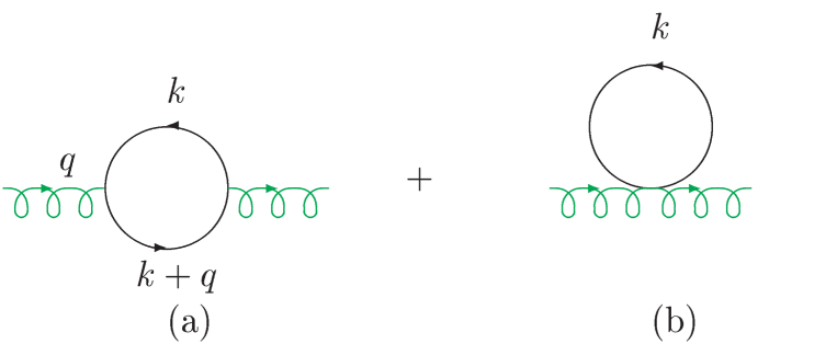
Figure 1: The scalar one-loop contribution to the graviton propagator. $q$ is the 4-momentum of the graviton.

In Ref. [6], we have shown that, while the naive power counting of the graphs gives their degree of divergence as +4, YFS [16] resummation of the soft graviton effects in the propagators in Fig. 1 renders the graphs ultra-violet (UV) finite. Indeed, for example, for Fig. 1a, we get without YFS resummation the result

$$i\Sigma(q)^{1a}_{\bar{\mu}\bar{\nu};\mu\nu}=\kappa^{2}\frac{\int d^{4}k}{2(2\pi)^{4}}\frac{\left(k^{\prime}_{\bar{\mu}}k_{\bar{\nu}}+k^{\prime}_{\bar{\nu}}k_{\bar{\mu}}\right)\left(k^{\prime}_{\mu}k_{\nu}+k^{\prime}_{\nu}k_{\mu}\right)}{\left({k^{\prime}}^{2}-m^{2}+i\epsilon\right)\left(k^{2}-m^{2}+i\epsilon\right)}$$ (3)

, where we set $k^{\prime}=k+q$ and we take for definiteness only fully transverse, traceless polarization states of the graviton to be act on $\Sigma$ so that we have dropped the traces from its vertices. Clearly, (3) has degree of divergence +4. When we take into account the resummation as calculated in Ref. [6], the free scalar propagators are improved to their YFS-resummed values,

$$i\Delta^{\prime}_{F}(k)|_{YFS-resummed}=\frac{ie^{B^{\prime\prime}_{g}(k)}}{(k^{2}-m^{2}+i\epsilon)}$$ (4)

, where the virtual graviton function $B^{\prime\prime}_{g}(k)$ is, for Euclidean momenta,

$$B^{\prime\prime}_{g}(k)=\frac{\kappa^{2}|k^{2}|}{8\pi^{2}}\ln\left(\frac{m^{2}}{m^{2}+|k^{2}|}\right),$$ (5)

so that we get instead of (3) the result ( here, $k\rightarrow(ik^{0},\vec{k})$ by Wick rotation )

$$i\Sigma(q)^{1a}_{\bar{\mu}\bar{\nu};\mu\nu}=i\kappa^{2}\frac{\int d^{4}k}{2(2\pi)^{4}}\frac{\left(k^{\prime}_{\bar{\mu}}k_{\bar{\nu}}+k^{\prime}_{\bar{\nu}}k_{\bar{\mu}}\right)e^{\frac{\kappa^{2}|{k^{\prime}}^{2}|}{8\pi^{2}}\ln\left(\frac{m^{2}}{m^{2}+|{k^{\prime}}^{2}|}\right)}\left(k^{\prime}_{\mu}k_{\nu}+k^{\prime}_{\nu}k_{\mu}\right)e^{\frac{\kappa^{2}|k^{2}|}{8\pi^{2}}\ln\left(\frac{m^{2}}{m^{2}+|k^{2}|}\right)}}{\left({k^{\prime}}^{2}-m^{2}+i\epsilon\right)\left(k^{2}-m^{2}+i\epsilon\right)}.$$ (6)

Evidently, this integral converges; so does that for Fig.1b when we use the improved resummed propagators. This means that we have a rigorous quantum loop correction to Newton’s law from Fig.1 which is finite and well defined.

To see how this result impacts the black hole character of our massive point particle, we continue to work in the transverse, traceless space for the graviton self-energy $\Sigma$ and we get, to leading order, that the graviton propagator denominator becomes

$$q^{2}+\frac{1}{2}q^{4}\Sigma^{T(2)}+i\epsilon$$ (7)

where the transverse, traceless self-energy function $\Sigma^{T}(q^{2})$ follows from eq.(6) for Fig. 1a and its analog for Fig. 1b by the standard methods. For the coefficient of $q^{4}$ in $\Sigma^{T}(q^{2})$ for $|q^{2}|>>m^{2}$ we have the result

$$-\frac{1}{2}\Sigma^{T(2)}\cong\frac{c_{2}}{360\pi M_{Pl}^{2}}$$ (8)

for

$$c_{2}=\int^{\infty}_{0}dxx^{3}(1+x)^{-4-\lambda_{c}x}\cong 72.1$$ (9)

where $\lambda_{c}=\frac{2m^{2}}{\pi M_{Pl}^{2}}$. When we Fourier transform the inverse of (7) we find the potential

$$\Phi_{Newton}(r)=-\frac{G_{N}M_{1}M_{2}}{r}(1-e^{-ar})$$ (10)

where $a=1/\sqrt{-\frac{1}{2}\Sigma^{T(2)}}\simeq 3.96M_{Pl}$ in an obvious notation, where for definiteness, we set $m\cong 120$GeV.

At this point, let us note that the integral in (9) can be represented for our purposes by the analytic expression [12]

$$c_{2}\cong\ln\frac{1}{\lambda_{c}}-\ln\ln\frac{1}{\lambda_{c}}-\frac{\ln\ln\frac{1}{\lambda_{c}}}{\ln\frac{1}{\lambda_{c}}-\ln\ln\frac{1}{\lambda_{c}}}-\frac{11}{6}$$ (11)

and we used this result to check the numerical result given in (9). It is clear that, without resummation, we would have $\lambda_{c}=0$ and our result in (9) would be infinite and, since this is the coefficient of $q^{4}$ in the inverse propagator, no renormalization of the field and of the mass could be used to remove such an infinity. In our new approach to quantum gravity, this infinity is absent.

We stress that our result in (8) is gauge invariant, as our approach involves the exact re-arrangement of the Feynman series as we explain in Ref. [6] and the original series is gauge invariant. Indeed, one can cross check this result by comparing with the pioneering work in Ref. [17], where the complete result of the one-loop divergences of our scalar field coupled to Einstein’s gravity have been computed. This is made possible by the following observation. As we just observed, the result which we have obtained would be UV divergent without our resummation. Thus, the dominant terms which we are isolating in this paper are precisely those that are given in Ref. [17], where we need to make the correspondence between the poles in $n$, the dimension of space-time, at $n=4$ calculated in Ref. [17] and the leading log $\ln\frac{1}{\lambda_{c}}$. This we do by setting the result $c_{2}$ equal to its value when $\lambda_{c}=0$ in $n$ dimensions and allowing $n\rightarrow 4$. In this way we find that

$$1/(2-n/2)\leftrightarrow c_{2}.$$ (12)

This means that, if we look at the limit $q^{2}\rightarrow 0$, we get the result that the coefficient of $q^{4}$ in (7) is $3/(2-n/2)$ times the coefficient of $c_{2}$ on the right-hand side of (8), and this is in complete agreement with the result that is implied by eq.(3.40) in Ref. [17], for example. Of course, the results in Ref. [17] are also gauge invariant.

In the SM, there are now believed to be three massive neutrinos [18], with masses that we estimate at $\sim 3$ eV, and the remaining members of the known three generations of Dirac fermions $\{e,\mu,\tau,u,d,s,c,b,t\}$, with masses given by  [19], $m_{e}\cong 0.51$ MeV, $m_{\mu}\cong 0.106$ GeV, $m_{\tau}\cong 1.78$ GeV, $m_{u}\cong 5.1$ MeV, $m_{d}\cong 8.9$ MeV, $m_{s}\cong 0.17$ GeV, $m_{c}\cong 1.3$ GeV, $m_{b}\cong 4.5$ GeV and $m_{t}\cong 174$ GeV, as well as the massive vector bosons $W^{\pm},~{}Z$, with masses $M_{W}\cong 80.4$ GeV, $M_{Z}\cong 91.19$ GeV. Using the general spin independence of the graviton coupling to matter at relatively low momentum transfers, we see that we can take the effects of these degrees of freedom into account approximately by counting each Dirac fermion as 4 degrees of freedom, each massive vector boson as 3 degrees of freedom and remembering that each quark has three colors. Using the result (11) for each of the massive degrees of freedom in the SM, we see that the effective value of $c_{2}$ in the SM is approximately

$$c_{2,eff}\cong 9.26\times 10^{3}$$ (13)

so that the effective value of $a$ in the SM is

$$a_{eff}\cong 0.349M_{Pl}.$$ (14)

To make direct contact with black hole physics, note that, for $r\rightarrow r_{S}$, $a_{eff}r\ll 1$ so that $|2\Phi_{Newton}(r)|_{M_{1}=m}/M_{2}|\ll 1$. This means that in the respective solution for our metric of space-time, $g_{00}\cong 1+2\Phi_{Newton}(r)|_{M_{1}=m}/M_{2}$ remains positive as we pass through the Schwarzschild radius. Indeed, it can be shown that this positivity holds to $r=0$. Similarly, $g_{rr}$ remains negative through $r_{S}$ down to $r=0$. To get these results, note that in the relevant regime for r, the smallness of the quantum corrected Newton potential means that we can use the linearized Einstein equations for a small spherically symmetric static source $\rho(r)$ which generates $\Phi_{Newton}(r)|_{M_{1}=m}/M_{2}$ via the standard Poisson’s equation. The usual result [20, 1, 2] for the respective metric solution then gives $g_{00}\cong 1+2\Phi_{Newton}(r)|_{M_{1}=m}/M_{2}$ and $g_{rr}\cong-1+2\Phi_{Newton}(r)|_{M_{1}=m}/M_{2}$ which remain respectively time-like and space-like to $r=0$.

It follows that the quantum corrections have obviated the classical conclusion that a massive point particle is a black hole [1].

We do not wish to suggest that the value of $a_{eff}$ given here is complete, as there may be as yet unknown massive particles beyond those already discovered. Including more particles in the computation of $a_{eff}$ would make it smaller and hence would not change the conclusions of our analysis. For example, in the Minimal Supersymmetric Standard Model we expect approximately that $a_{eff}\rightarrow\frac{1}{\sqrt{2}}a_{eff}$. In addition, we point-out that, using the correspondence in (12) one can also use the results for the complete one-loop corrections in Ref. [17] to the theory treated here to see that the remaining interactions at one-loop order not discussed here (vertex corrections, pure gravity self-energy corrections, etc. ) also do not increase the value of $a_{eff}$ [21]. We can thus think of $a_{eff}$ as a parameter which is bounded from above by the estimates we give above and which should be determined from cosmological and/or other considerations. Further such implications will be taken up elsewhere.

References

- [1] C. Misner, K.S. Thorne and J.A. Wheeler, Gravitation,( Freeman, San Francisco, 1973 ).
- [2] S. Weinberg, Gravitation and Cosmology: Principles and Applications of the General Theory of Relativity,( John Wiley, New York, 1972).
- [3] See, for example, M. Green, J. Schwarz and E. Witten, Superstring Theory, v. 1 and v.2, ( Cambridge Univ. Press, Cambridge, 1987 ) and references therein.
- [4] See, for example, J. Polchinski, String Theory, v. 1 and v. 2, (Cambridge Univ. Press, Cambridge, 1998), and references therein.
- [5] S.L. Glashow, Nucl. Phys. 22 (1961) 579; S. Weinberg, Phys. Rev. Lett. 19 (1967) 1264; A. Salam, in Elementary Particle Theory, ed. N. Svartholm (Almqvist and Wiksells, Stockholm, 1968), p. 367; G. ’t Hooft and M. Veltman, Nucl. Phys. B44,189 (1972) and B50, 318 (1972); G. ’t Hooft, ibid. B35, 167 (1971); M. Veltman, ibid. B7, 637 (1968); D. J. Gross and F. Wilczek, Phys. Rev. Lett. 30 (1973) 1343; H. David Politzer, ibid.30 (1973) 1346; see also , for example, F. Wilczek, in Proc. 16th International Symposium on Lepton and Photon Interactions, Ithaca, 1993, eds. P. Drell and D.L. Rubin (AIP, NY, 1994) p. 593, and references therein.
- [6] B.F.L. Ward, Mod. Phys. Lett. A17 (2002) 2371.
- [7] S. Hawking, Nature ( London ) 248 (1974) 30; Commun. Math. Phys. 43 ( 1975 ) 199.
- [8] R. P. Feynman, Acta Phys. Pol. 24 (1963) 697.
- [9] R. P. Feynman, Feynman Lectures on Gravitation, eds. F.B. Moringo and W.G. Wagner (Caltech, Pasadena, 1971).
- [10] D. Bardin and G. Passarino,The Standard Model in the Making : Precision Study of the Electroweak Interactions , ( Oxford Univ. Press, London, 1999 ).
- [11] M.L. Goldberger, private communication, 1972.
- [12] B.F.L. Ward, to appear.
- [13] D. Abbaneo et al., hep-ex/0212036; see also, M. Gruenewald, hep-ex/0210003, in Proc. ICHEP02, in press, 2003.
- [14] S. Perlmutter et al., Astrophys. J. 517 (1999) 565; and, references therein.
- [15] L. D. Faddeev and V.N. Popov, ITF-67-036, NAL-THY-57 (translated from Russian by D. Gordon and B.W. Lee); Phys. Lett. B25 (1967) 29.
-
[16]
D. R. Yennie, S. C. Frautschi, and H. Suura, Ann. Phys. 13 (1961) 379;
see also K. T. Mahanthappa, Phys. Rev. 126 (1962) 329, for a related analysis. - [17] G. ’t Hooft and M. Veltman, Ann. Inst. Henri Poincare XX, 69 (1974).
- [18] See for example D. Wark, in Proc. ICHEP02, in press; and, M. C. Gonzalez-Garcia, hep-ph/0211054, in Proc. ICHEP02, in press, and references therein.
- [19] K. Hagiwara et al., Phys. Rev. D66 (2002) 010001; see also H. Leutwyler and J. Gasser, Phys. Rept. 87 (1982) 77, and references therein.
- [20] R. Adler, M. Bazin and M. Schiffer, Introduction to General Relativity ,( McGraw-Hill, New York, 1965 ).
- [21] B.F.L. Ward, to appear.