$\phi\rightarrow KK$ decay in light cone QCD

The coupling constant of $\phi\rightarrow KK$ decay is calculated in light cone QCD sum rules. The result obtained for $g_{\phi KK}=(4.9\pm 0.8)$ is in a good agreement with the existing experimental result.

PACS numbers: 11.50.Hx, 13.25.Jx

1 Introduction

Light scalar mesons constitute a remarkable exception of the quark model systematization of mesons and their nature still need to be unambiguously established [1].

Particularly, the nature $f_{0}(980)$ meson is under debate. According to the naive $\bar{q}q$ picture and strong coupling with kaons, $f_{0}(980)$ can be interpreted as a pure $\bar{s}s$ state [2]–[4]. However, this interpretation does not explain mass degeneracy between $f_{0}(980)$ and isovector $a_{0}(980)$, which is interpreted as a ($\bar{u}u-\bar{d}d)/\sqrt{2}$ state. It is also interpreted as a four quark $\bar{q}q\bar{s}s$ [5] bound state of hadrons [6]–[8] and as a result of a process known as hadronic dressing [2, 9].

For understanding the content of the $f_{0}$ meson several alternatives have been suggested: For example, analysis of $\phi\rightarrow f_{0}\gamma$ decay [5]–[10] and investigation of the ratio $\Gamma(a_{0}\rightarrow f_{0}\gamma)/\Gamma(\phi\rightarrow f_{0}\gamma)$ [7, 8] are believed to be the most promising ones for this purpose.

The $\phi\rightarrow f_{0}\gamma$ decay is a very efficient tool for this purpose, since the branching ratio is essentially dependent on the content of $f_{0}$. For example, if $f_{0}$ is a pure $\bar{s}s$ state, the branching ratio is $\sim 10^{-5}$, while if $f_{0}$ is composed of four quarks then the branching ratio is expected to be $\sim 10^{-4}$.

The strong coupling constants $g_{\phi K^{+}K^{-}}$ and $g_{f_{0}K^{+}K^{-}}$ are among the important hadronic parameters entering to the analysis involving $\phi$ and $f_{0}(980)$. Indeed, the kaon loop diagrams contributing $\phi\rightarrow f_{0}\gamma$ are expected to be in terms of $g_{f_{0}K^{+}K^{-}}$, as well as $g_{\phi K^{+}K^{-}}$. The coupling constant $g_{f_{0}K^{+}K^{-}}$ is studied in light cone QCD sum rules [10] (more about light cone QCD sum rules and and its applications can be found in [11, 12]).

In the present work we calculate the strong coupling constant $g_{\phi K^{+}K^{-}}$ in light cone QCD sum rules method. It should be noted that this constant can be obtained from experimental data on $\phi$ meson decays. The goal in the present work is twofold: Firstly, can we get new information about the quark content of $\phi$ meson comparing experimental data with theoretical results? Secondly, how does light cone QCD work for the asymmetric case, i.e., with different Borel mass parameters corresponding to different mass channels?

The paper is organized as follows. In section 2, we derive sum rules for the $g_{\phi K^{+}K^{-}}$ coupling constant. In section 3, we present our numerical results and conclusion.

2 Sum rules for $g_{\phi K^{+}K^{-}}$ coupling constant

In this section we calculate the strong coupling constant $g_{\phi K^{+}K^{-}}$ in light cone QCD sum rules. This coupling constant is defined by the following matrix element:

$$\langle K^{-}(q)\phi^{0}(p,\varepsilon)|K^{+}(p+q)\rangle~{},$$ (1)

where the momentum assignment is specified in brackets and $\varepsilon_{\mu}$ is the polarization vector of the $\phi$ meson. In order to calculate the strong coupling constant $g_{\phi K^{+}K^{-}}$ we consider the following correlator function

$$\Pi_{\mu\nu}(p,q)=i\int d^{4}xe^{ipx}\left<K(q)\left|\mbox{\rm T}\left\{J_{\nu}^{\phi}(x)\bar{J}_{\mu}^{K}(0)\right\}\right|0\right>~{},$$ (2)

where the quark current $J_{\mu}^{K}=\bar{u}\gamma_{\mu}\gamma_{5}s$ is the axial vector current and $J_{\nu}^{\phi}=\bar{s}\gamma_{\mu}s$ is the interpolating current for the $\phi$ meson.

The correlator function, in general, can be written in terms of the following five independent invariant functions

$$\Pi_{\mu\nu}(p,q)=\Pi_{1}g_{\mu\nu}+\Pi_{2}p_{\mu}p_{\nu}+\Pi_{3}p_{\mu}q_{\nu}+\Pi_{4}q_{\mu}p_{\nu}+\Pi_{5}q_{\mu}q_{\nu}~{}.$$ (3)

Therefore, our first problem is to choose the kinematical structure. For this aim, we consider the phenomenological part of the correlator function. This part can be written as

$$\Pi_{\mu\nu}=\sum\frac{\langle K^{-}(q)\phi^{0}(p)|K^{+}(p+q)\rangle\langle K^{+}(p+q)|J_{\mu}^{K}|0\rangle\langle 0|J_{\nu}^{\phi}|\phi(p)\rangle}{(p^{2}-m_{\phi}^{2})[(p+q)^{2}-m_{K}^{2}]}~{}.$$ (4)

The matrix elements entering Eq. (4) are defined as

$$\langle K^{+}(p+q)|J_{\mu}^{K}|0\rangle\!\!\! = \!\!\!f_{K}(p+q)_{\mu}~{},$$

$$\langle 0|J_{\nu}^{\phi}|\phi(p)\rangle\!\!\! = \!\!\!m_{\phi}f_{\phi}\varepsilon_{\nu}~{}.$$ (5)

Using Eqs. (4) and (2), we get for the physical part

$$\Pi_{\mu\nu}=\frac{g_{\phi K^{+}K^{-}}f_{K}m_{\phi}f_{\phi}}{(p^{2}-m_{\phi}^{2})[(p+q)^{2}-m_{K}^{2}]}\,(p_{\mu}+q_{\mu})\left(q_{\nu}+\frac{1}{2}p_{\nu}\right)~{}.$$ (6)

It follows from this expression that the only the structures $p_{\mu}q_{\nu}$, $q_{\mu}q_{\nu}$, $q_{\mu}p_{\nu}$ and $p_{\mu}p_{\nu}$ give contribution to the correlator function. In further analysis, we will choose the structure $p_{\mu}q_{\nu}$ from which the corresponding invariant structure

$$\Pi=\frac{g_{\phi K^{+}K^{-}}f_{K}m_{\phi}f_{\phi}}{(p^{2}-m_{\phi}^{2})[(p+q)^{2}-m_{K}^{2}]}~{},$$ (7)

follows.

Our next task is the calculation of the correlator function from QCD side. This calculation can be carried out by using light cone operator product expansion method, in which we work with large momenta, i.e., $-p^{2}$ and $-(p+q)^{2}$ are both large. The correlator function, then, can be calculated as an expansion near to the light cone $x^{2}\simeq 0$. The expansion involves matrix elements of the nonlocal operators between vacuum and the kaon states, i.e., in terms of kaon wave functions with increasing twist.

After lengthy calculations, we get the following expression for the invariant function which is proportional to the structure $p_{\mu}q_{\nu}$

$$\Pi(p^{2},(p+q)^{2})=if_{K}\int_{0}^{1}du\Bigg{\{}\frac{4ug_{2}(u)}{\Delta^{2}}+\frac{\varphi_{K}(u)}{\Delta}-4\frac{g_{1}(u)+G_{2}(u)}{\Delta^{2}}\left(1+\frac{2m_{s}^{2}}{\Delta}\right)$$ (8)

$$+ \!\!\!\frac{m_{K}^{2}}{3}\frac{\varphi_{\sigma}(u)}{\Delta^{2}}\Bigg{\}}+if_{K}\int_{0}^{1}du\,u\int{\cal D}\alpha_{i}\frac{2}{\Delta_{2}^{2}}\Big{[}2\varphi_{\perp}(\alpha_{i})+\varphi_{\parallel}+2\tilde{\varphi}_{\perp}(\alpha_{i})\Big{]}$$

$$+ \!\!\!if_{K}\int_{0}^{1}du\int_{0}^{1}d\alpha_{3}\int_{0}^{1-\alpha_{3}}d\alpha_{1}\frac{1}{\Delta_{2}^{2}}\Big{[}2\varphi_{\perp}(\alpha_{i})-\varphi_{\parallel}+2\tilde{\varphi}_{\perp}(\alpha_{i})-\tilde{\varphi}_{\parallel}(\alpha_{i})\Big{]}$$

$$+ \!\!\!2if_{K}\Bigg{\{}\int_{0}^{1}du(u-1)\int_{0}^{1}d\alpha_{3}\frac{4\hat{F}(\alpha_{3})\{pq+m_{K}^{2}[1+\alpha_{3}(u-1)]\}}{\Delta_{1}^{3}}$$

$$+ \!\!\!\int_{0}^{1}du\int_{0}^{1}d\alpha_{3}\int_{0}^{1-\alpha_{3}}d\alpha_{1}\frac{4F(\alpha_{i})[pq+m_{K}^{2}(\alpha_{1}+u\alpha_{3})]}{\Delta_{2}^{3}}~{}\Bigg{\}},$$

where

$$\Delta\!\!\! = \!\!\!m_{s}^{2}-(p+qu)^{2}~{},$$

$$\Delta_{1}\!\!\! = \!\!\!m_{s}^{2}-[p+q(1+(u-1)\alpha_{3}]^{2}~{},$$

$$\Delta_{2}\!\!\! = \!\!\!m_{s}^{2}-[p+q(\alpha_{1}+u\alpha_{3})]^{2}~{},$$ (9)

and,

$$\hat{F}(\alpha_{3})\!\!\! = \!\!\!-\int_{0}^{\alpha_{3}}dt\int_{0}^{1-t}d\alpha_{1}\Phi(\alpha_{1},1-\alpha_{1}-t,t)~{},$$ (10)

$$F(\alpha_{i})\!\!\! = \!\!\!-\int_{0}^{\alpha_{1}}dt\Phi(t,1-\alpha_{3}-t,\alpha_{3})~{},$$ (11)

$$\Phi(\alpha_{i})\!\!\! = \!\!\!\varphi_{\parallel}(\alpha_{i})+\varphi_{\perp}(\alpha_{i})+\tilde{\varphi}_{\parallel}(\alpha_{i})+\tilde{\varphi}_{\perp}(\alpha_{i})~{}.$$ (12)

The functions in Eq. (8) are defined as

$$\langle K(q)|\bar{u}(x)\gamma_{\mu}\gamma_{5}s(0)|0\rangle\!\!\! = \!\!\!-if_{K}q_{\mu}\int_{0}^{1}due^{iuqx}[\varphi_{K}(u)+x^{2}g_{1}(u)]$$ (13)

$$+ \!\!\!f_{K}\left(x_{\mu}-\frac{q_{\mu}x^{2}}{qx}\right)\int_{0}^{1}due^{iuqx}g_{2}(u)~{},$$

$$\langle K(q)|\bar{u}(x)\sigma_{\mu\nu}\gamma_{5}s(0)|0\rangle\!\!\! = \!\!\!i(q_{\mu}x_{\nu}-q_{\nu}x_{\mu})\frac{f_{K}m_{K}^{2}}{6m_{s}}\int_{0}^{1}due^{iuqx}\varphi_{\sigma}(u)~{},$$ (14)

and

$$G(u)=-\int_{0}^{u}g_{2}(u)dv~{}.$$ (15)

The matrix elements involving quark–gluon field are determined as

$$\langle K(q)|\bar{u}(x)\gamma_{\mu}\gamma_{5}g_{s}G_{\alpha\beta}(ux)s(0)|0\rangle=$$ (16)

$$f_{K}\Bigg{[}q_{\beta}\left(g_{\alpha\mu}-\frac{x_{\alpha}q_{\mu}}{qx}\right)-q_{\beta}\left(g_{\beta\mu}-\frac{x_{\beta}q_{\mu}}{qx}\right)\Bigg{]}\int{\cal D}\alpha_{i}\varphi_{\perp}(\alpha_{i})e^{iqx(\alpha_{1}+u\alpha_{3})}$$

$$+ \!\!\!f_{K}\frac{q_{\mu}}{qx}\left(q_{\alpha}x_{\beta}-q_{\beta}x_{\alpha}\right)\int{\cal D}\alpha_{i}\varphi_{\parallel}(\alpha_{i})e^{iqx(\alpha_{1}+u\alpha_{3})}$$

$$\langle K(q)|\bar{u}(x)\gamma_{\mu}g_{s}\tilde{G}_{\alpha\beta}(ux)s(0)|0\rangle=$$ (17)

$$if_{K}\Bigg{[}q_{\beta}\left(g_{\alpha\mu}-\frac{x_{\alpha}q_{\mu}}{qx}\right)-q_{\beta}\left(g_{\beta\mu}-\frac{x_{\beta}q_{\mu}}{qx}\right)\Bigg{]}\int{\cal D}\alpha_{i}\tilde{\varphi}_{\perp}(\alpha_{i})e^{iqx(\alpha_{1}+u\alpha_{3})}$$

$$+ \!\!\!if_{K}\frac{q_{\mu}}{qx}\left(q_{\alpha}x_{\beta}-q_{\beta}x_{\alpha}\right)\int{\cal D}\alpha_{i}\tilde{\varphi}_{\parallel}(\alpha_{i})e^{iqx(\alpha_{1}+u\alpha_{3})}~{},$$

where $\tilde{G}_{\alpha\beta}=\frac{1}{2}\epsilon_{\alpha\beta\rho\sigma}G^{\rho\sigma}$, ${\cal D}\alpha_{i}=d\alpha_{1}d\alpha_{2}d\alpha_{3}\delta(1-\alpha_{1}-\alpha_{2}-\alpha_{3})$.

The sum rule for $g_{\phi K^{+}K^{-}}$ is obtained by equating the phenomenological, Eq. (7), and theoretical, Eq. (8), parts.

In order to suppress the contributions of the continuum and higher states, we perform double Borel transformation over the variables $-p^{2}$ and $-(p+q)^{2}$ on both sides of Eqs. (7) and (8), and obtain the following expression for the correlator function

$$f_{K}m_{\phi}f_{\phi}g_{\phi KK}e^{-m_{p}hi^{2}/M_{1}^{2}}e^{-m_{K}^{2}/M_{2}^{2}}=f_{K}e^{-m_{0}^{2}/M^{2}}\Bigg{\{}M^{2}\varphi_{K}(u_{0})+4u_{0}g_{2}(u_{0})$$ (18)

$$- \!\!\!4[g_{1}(u_{0})+G_{2}(u_{0})]+\frac{m_{K}^{2}}{3}\varphi_{\sigma}(u_{0})-4\frac{m_{s}^{2}}{M^{2}}[g_{1}(u_{0})+G_{2}(u_{0})]+\Bigg{(}\int_{0}^{1-u_{0}}d\alpha_{3}\int_{u_{0}-\alpha_{3}}^{u_{0}}d\alpha_{1}$$

$$+ \!\!\!\int_{1-u_{0}}^{1}d\alpha_{3}\int_{u_{0}-\alpha_{3}}^{1-\alpha_{3}}d\alpha_{1}-\int_{u_{0}}^{1}d\alpha_{3}\int_{u_{0}-\alpha_{3}}^{0}d\alpha_{1}\Bigg{)}\Bigg{(}2\frac{u_{0}-\alpha_{1}}{\alpha_{3}}\,\frac{2\varphi_{\perp}(\alpha_{i})+\varphi_{\parallel}(\alpha_{i})+2\tilde{\varphi}_{\perp}(\alpha_{i})}{\alpha_{3}}$$

$$+ \!\!\!\frac{\Phi(\alpha_{i})}{\alpha_{3}}-\frac{2}{\alpha_{3}}\frac{dF(\alpha_{i})}{d\alpha_{1}}\Bigg{)}-2\int_{1-u_{0}}^{1}\frac{\hat{F}^{\prime}(\alpha_{3})}{\alpha_{3}}d\alpha_{3}-2\int_{1-u_{0}}^{1}d\alpha_{3}\frac{F(1-\alpha_{3},0,\alpha_{3})}{\alpha_{3}}\Bigg{\}}~{},$$

where

$$M^{2}=\frac{M_{1}^{2}M_{2}^{2}}{M_{1}^{2}+M_{2}^{2}}~{},~{}~{}~{}~{}~{}u_{0}=\frac{M_{1}^{2}}{M_{1}^{2}+M_{2}^{2}}~{},~{}~{}~{}~{}\mbox{and},~{}~{}~{}~{}~{}m_{0}^{2}=m_{s}^{2}+m_{K}^{2}u_{0}(1-u_{0})~{}.$$

Subtraction of the continuum and higher states is carried out by employing the quark–hadron duality, i.e., continuum contribution, which is represented in terms of the spectral density obtained from QCD side, by equating it to the one obtained from QCD side, but starting from some given threshold. The prescription for subtraction the contribution of the continuum in light cone version of the sum rule is proposed in [13] (see also [14]). In [13] and in many works, the symmetric point $M_{1}^{2}=M_{2}^{2}=2M^{2}$ (i.e., $u_{0}=1/2$) is considered, and then the continuum subtraction is implemented by means of the simple substitution

$$e^{-m^{2}/M^{2}}\rightarrow e^{-m^{2}/M^{2}}-e^{-s_{0}/M^{2}}~{},$$

in the leading twist term (in our case leading twist term is the wave function $\varphi_{K}(u)$). But this prescription is not adequate in our case, where the Borel parameters and masses of different channels are not equal. In the present work we will follow the analysis given in [10], where the prescription for continuum subtraction through use of the Borel parameters with different masses in the respective channels is proposed, and properties of the wave functions are exploited. Namely, the leading twist–2 wave function can be exploited as a power series

$$\varphi_{K}(u)=\sum_{k}b_{k}(1-u)^{k}~{},$$

in order to calculate its contribution in the duality region. Here we will neglect the continuum subtraction in the higher twist terms altogether, due to their small contribution to the theoretical part of the sum rules. Here, we will neglect the continuum subtraction in all higher twist terms, due to their small contribution to the theoretical part of the sum rules.

The final result for the $g_{\phi KK}$ coupling is given as

$$g_{\phi KK}=\frac{1}{m_{\phi}f_{\phi}}e^{m_{\phi}^{2}/M_{1}^{2}}e^{m_{K}^{2}/M_{2}^{2}}e^{-m_{0}^{2}/M^{2}}\Bigg{\{}M^{2}\sum_{k}b_{k}\left(\frac{M^{2}}{M_{1}^{2}}\right)^{k}\Bigg{[}1-e^{-(s_{0}-m_{s}^{2})/M^{2}}\sum_{i=0}^{k}\frac{1}{i!}\left(\frac{s_{0}-m_{s}^{2}}{M^{2}}\right)^{i}$$ (19)

$$+ \!\!\!e^{-(s_{0}-m_{s}^{2})/M^{2}}\frac{m_{K}^{2}M^{2}}{M_{1}^{2}M_{2}^{2}}\frac{1}{(k+1)!}\left(\frac{s_{0}-m_{s}^{2}}{M^{2}}\right)^{k+1}\Bigg{]}+4u_{0}g_{2}(u_{0})-4[g_{1}(u_{0})+G_{2}(u_{0})]$$

$$+ \!\!\!\frac{m_{K}^{2}}{3}\varphi_{\sigma}(u_{0})-4\frac{m_{s}^{2}}{M^{2}}[g_{1}(u_{0})+G_{2}(u_{0})]+\Bigg{(}\int_{0}^{1-u_{0}}d\alpha_{3}\int_{0}^{u_{0}}d\alpha_{1}+\int_{1-u_{0}}^{1}d\alpha_{3}\int_{u_{0}-\alpha_{3}}^{1-\alpha_{3}}d\alpha_{1}$$

$$- \!\!\!\int_{u_{0}}^{1}d\alpha_{3}\int_{u_{0}-\alpha_{3}}^{0}d\alpha_{1}\Bigg{)}\Bigg{[}2\frac{u_{0}-\alpha_{1}}{\alpha_{3}^{2}}\Big{(}2\varphi_{\perp}(\alpha_{i})+\varphi_{\parallel}(\alpha_{i})+2\tilde{\varphi}_{\perp}(\alpha_{i})\Big{)}+\frac{\Phi(\alpha_{i})}{\alpha_{3}}-\frac{2}{\alpha_{3}}\frac{dF(\alpha_{i})}{d\alpha_{1}}\Bigg{]}$$

$$- \!\!\!2\int_{1-u_{0}}^{1}{d\alpha_{3}}\frac{\hat{F}^{\prime}(\alpha_{3})}{\alpha_{3}}-2\int_{1-u_{0}}^{1}{d\alpha_{3}}\frac{F(1-\alpha_{3},0,\alpha_{3})}{\alpha_{3}}\Bigg{\}}~{},$$

where $s_{0}$ is the smallest continuum contribution.

3 Numerical analysis

In this section we present our numerical calculation on $g_{\phi KK}$ coupling constant. It follows from Eq. (19) that the main input parameters are the kaon wave functions. The theoretical framework for their determination is based on an expansion in terms of the matrix elements of conformal operators [15]. In particular, for the leading twist–2 wave function $\varphi_{K}(u)$ defined in Eq. (13), the expansion goes into Gegenbauer polynomials:

$$\varphi_{K}(u,\mu^{2})=6u(1-u)\Bigg{[}1+\sum_{n=1}^{\infty}a_{2n}(\mu^{2})C_{2n}^{3/2}(2u-1)\Bigg{]}~{},$$ (20)

where $a_{2}(1~{}GeV)=0.2$ [16].

Analogously $\varphi_{\sigma}$ is defined as

$$\varphi_{\sigma}(u)=6u(1-u)\Bigg{[}1+\left(5\eta_{3}-\frac{1}{2}\eta_{3}w_{3}-\frac{7}{20}\rho^{2}-\frac{3}{5}\rho^{2}\tilde{a}_{2}\right)C_{2}^{3/2}(2u-1)+\cdots\Bigg{]}~{},$$ (21)

where, at the $\mu=1~{}GeV$ scale $\eta_{3}=0.015$, $w_{3}=-3$, $\tilde{a}_{2}=0.2$. Here, the factor $\rho=m_{s}^{2}/m_{K}^{2}$ takes into account the boson mass corrections (see [17]). The twist–4 wave functions $\varphi_{\parallel}(\alpha_{i})$, $\varphi_{\perp}(\alpha_{i})$, $\tilde{\varphi}_{\parallel}(\alpha_{i})$ and $\tilde{\varphi}_{\perp}(\alpha_{i})$, including the meson mass corrections are given as (see [15] and [17])

$$\varphi_{\perp}(\alpha_{i})\!\!\! = \!\!\!30m_{K}^{2}\alpha_{3}^{2}(2\alpha_{1}-1-\alpha_{3})\Bigg{[}h_{00}+h_{01}\alpha_{3}+\frac{h_{10}}{2}(5\alpha_{3}-3)+\cdots\Bigg{]}$$

$$\varphi_{\perp}(\alpha_{i})\!\!\! = \!\!\!120m_{K}^{2}\alpha_{1}(1-\alpha_{1}-\alpha_{3})\alpha_{3}[a_{10}(1-2\alpha_{1}-\alpha_{3})+\cdots\Bigg{]}~{},$$

$$\tilde{\varphi}_{\perp}(\alpha_{i})\!\!\! = \!\!\!-30m_{K}^{2}\alpha_{3}^{2}\Bigg{\{}h_{00}(1-\alpha_{3})+h_{01}[\alpha_{3}(1-\alpha_{3})+6\alpha_{1}(1-\alpha_{1}-\alpha_{3})$$

$$+ \!\!\!h_{10}[\alpha_{3}(1-\alpha_{3})-\frac{3}{2}[\alpha_{1}^{2}+(1-\alpha_{1}-\alpha_{3})^{2}]+\cdots\Bigg{\}}~{},$$

$$\tilde{\varphi}_{\perp}(\alpha_{i})\!\!\! = \!\!\!120m_{K}^{2}\alpha_{1}(1-\alpha_{1}-\alpha_{3})\alpha_{3}[v_{00}+v_{10}(3\alpha_{3}-1)+\cdots\Bigg{]}~{},$$

where

$$h_{00}\!\!\! = \!\!\!v_{00}=-\frac{1}{3}\eta_{4}~{},$$

$$h_{01}\!\!\! = \!\!\!\frac{7}{4}\eta_{4}w_{4}-\frac{3}{20}a_{2}~{},$$

$$h_{10}\!\!\! = \!\!\!\frac{7}{2}\eta_{4}w_{4}+\frac{3}{20}a_{2}~{},$$

$$v_{10}\!\!\! = \!\!\!\frac{21}{8}\eta_{4}w_{4}~{},$$

$$a_{10}\!\!\! = \!\!\!\frac{21}{8}\eta_{4}w_{4}-\frac{9}{20}a_{2}~{},$$

with $\eta_{4}(\mu=1~{}GeV)=0.6$ and $w_{4}(\mu=1~{}GeV)=0.2$ [15, 17].

The values of other input parameters appearing in Eq. (19) are: $m_{s}=0.14~{}GeV$ [18], $m_{K}=0.4937~{}GeV$, $m_{\phi}=1.02~{}GeV$. Leptonic decay constant of $\phi$ meson, $f_{\phi}=0.234~{}GeV$, follows from the experimental result of the $\phi\rightarrow\ell^{+}\ell^{-}$ decay [19]. The threshold $s_{0}$ which is varied around the value $s_{0}=1.1~{}GeV^{2}$, is determined from the analysis of two–point function sum rules for $f_{K}$ [20].

Having all input parameters, we now proceed by carrying out numerical calculation. The dependence of $g_{\phi KK}$ on Borel masses $M_{1}^{2}$ and $M_{2}^{2}$ at two fixed values of $s_{0}=1.1~{}GeV^{2}$ and $s_{0}=1.2~{}GeV^{2}$ is presented in Figs. (1) and (2), respectively. According to the QCD sum rule method ranges of the auxiliary Borel parameters $M_{i}^{2}$ should be found such that the result for $g_{\phi KK}$ be practically independent of them.

From these figures we see that, such regions indeed do exist. When $M_{1}^{2}$ and $M_{2}^{2}$ are varied in the regions $2~{}GeV^{2}\leq M_{1}^{2}\leq 4~{}GeV^{2}$ and $0.8~{}GeV^{2}\leq M_{2}^{2}\leq 1.4~{}GeV^{2}$, the result for $g_{\phi KK}$ seems to be independent of the Borel parameters. It should be noted here that, the result changes slightly when the continuum threshold is fixed to the value $s_{0}=1.2~{}GeV^{2}$. The final result for $g_{\phi KK}$ is

$$g_{\phi KK}=4.9\pm 0.8~{}.$$ (22)

At this point, let us discuss sources of the uncertainties. $SU_{f}(3)$ breaking effects in kaon distribution amplitudes which we neglected, can play essential role, since we can explore wide range of $u$ and hence smoothing the effects of the shape of wave function. Additional uncertainty arises from the value of $m_{s}$. All these factors can cause an uncertainty about 5–10%. Moreover, the errors coming from the variations in the continuum threshold and Borel masses, change the result about 10%. If all these uncertainties are taken into account, the resulting error is about 20%, which is quoted in Eq. (22).

Finally, we would comment that, existing experimental results on $\phi\rightarrow KK$ decay predicts $g_{\phi KK}=4.8$. So, obviously, we see that our result is quite close to the experimental value. Therefore we conclude that the quark content of $\phi$ is $\bar{s}s$, and for channels with different masses and different Borel parameters, light cone QCD sum rules work quite well.

Figure captions

Fig. (1) The dependence of the coupling constant $g_{\phi KK}$ on the Borel parameters $M_{1}^{2}$ and $M_{2}^{2}$, at the fixed value $s_{0}=1.1~{}GeV^{2}$ of the continuum threshold.

Fig. (2) The same as Fig. (1), but at the fixed value $s_{0}=1.2~{}GeV^{2}$ of the continuum threshold.

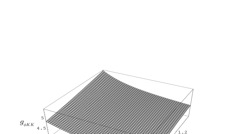
Figure 1:

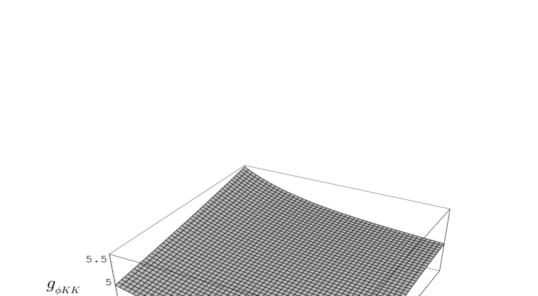
Figure 2: