Nonperturbative contributions to the quark form factor at high energy

Abstract

The analysis of nonperturbative effects in high energy asymptotics of the electomagnetic quark form factor is presented. It is shown that the nonperturbative effects determine the initial value for the perturbative evolution of the quark form factor and find their general structure with respect to the high energy asymptotics. Within the Wilson integral formalism which is natural for investigation of the soft, IR sensitive, part of the factorized form factor, the structure of the instanton induced effects in the evolution equation is discussed. It is demonstrated that the instanton contributions result in the finite renormalization of the subleading perturbative result and numerically are characterized by small factor reflecting the diluteness of the QCD vacuum within the instanton liquid model. The relevance of the IR renormalon induced effects in high energy asymptotic behaviour is discussed. The consequences of the various analytization procedures of the strong coupling constant in the IR domain are considered.

I Introduction

The electromagnetic (color singlet) quark form factor is one of the simplest and convenient objects for the investigation of the double logarithmic behaviour of the QCD amplitudes in the high energy regime. From the methodological point of view, the consistent study of such an asymptotic requires a perturbative resummation procedure beyond the standard renormalization group techniques. Besides this, the resummation methods developed for this particular case can be applied to study of many other processes which possess the logarithmic enhancements near the kinematic boundaries. On the other hand, in addition to the evident theoretical significance, the computation of the quark form factors has important phenomenological applications. The quark form factor enters into the cross sections of a number of the high energy hadronic processes HARD . For example, the total cross section of the Drell-Yan process (normalized to DIS) is determined by the ratio of the time-like and space-like form factors PAR ; MAG . The similar resummation approach is used also in study of the near-forward quark-quark scattering, and evaluation of the soft Pomeron properties KRP . In the latter case, the nonleading logarithmic terms are quite important. The investigation of the electomagnetic quark form factors (Dirac as well as Pauli) in moderate and low energy domains can shed a light on the problem of the scaling violation in DIS and the structure of constituent quarks SCAL .

The first example of the large logarithm resummation was given by Sudakov for the case of off-shell fermion in external Abelian gauge field in the leading logarithmic approximation (LLA), where the terms of order of $(\alpha_{s}^{n}\ln^{2n}q^{2})$ are taken into account while the contributions from $O(\alpha_{s}^{n}\ln^{2n-1}q^{2})$ are neglected. The exponentiation of the leading double logarithmic result was found SUD . This exponential decreasing of the form factor at large-$q^{2}$ means that the elastic scattering of a quark by a virtual photon is suppressed at asymptotically large momentum transfer. The exponentiation for the on-shell form factor in the Abelian case was obtained in the LLA in ONLLA . As expected, the non-Abelian gauge theories appeared to be more complicated: first, the leading LLA terms in the QCD perturbative series were found to be consistent with exponentiation in LLANA (the inelastic on-shell form factor with emission of one and two gluons was calculated in the same context in LLANAIE ; the role of the quark Sudakov form factor in the description of $e^{+}e^{-}$ one-photon annihilation in quarks and gluons was considered in LLA in FEL ), and the all-order LLA non-Abelian exponentiation has been proved in LLAAOR . In the LLA, the exponentiated form factor was shown to be the rapidly decreasing function at high momentum transfer, but the question if the non-leading logarithmic terms could upset the LLA behaviour required a further work. The all-(logarithmic)-order resummation was performed in the Abelian case and the exponentiation was demonstrated in ALLLOGA . In the paper ALLLOGNA , the non-Abelian all-order exponentiation for the so-called hard part of the on-shell form factor has been shown first within the powerful factorization approach. Note, that in this work the case where a time-like photon with large invariant mass decays into a quark-antiquark pair was considered, however it can be easily shown that the results remain true for our case of a quark scattering in an external EM field as well.

In the work ALLLOGNA , the detailed study of hard part of the form factor (which is responsible for the UV properties) was performed, while the status of the soft part, containing all the IR and collinear singularities and, as a consequence, all possible nonperturbative effects, remained unclear. The important results on the IR properties of the QCD vertex functions was obtained in KRC1 within the Wilson integral approach. In these works, the soft part of the form factor had been presented as the vacuum averaged ordered exponent of the path integral of a gauge field over the contour of a special form—an angle with sides of infinite length. The use of the gauge and renormalization group invariance allowed to derive the perturbative evolution equation describing the high energy behaviour of the form factor taking into account all (not power suppressed) parts of the factorized amplitude, both for the on- KRON and off-shell KROFF cases. It was shown that the leading asymptotic is controlled by the cusp anomalous dimension which arises due to the multiplicative renormalization of the soft part, and can be calculated within the Wilson integral formalism up to the two-loop order KRC1 . It is worth noting that within the Wilson integral approach, the non-Abelian exponentiation can be proved independently NAEXP , what is another important advantage of this framework. The efficiency of the Wilson integrals approach had been successfully demonstrated in a series of works STEF1 ; STEF2 ; STEF3 . In these papers, the consistent non-diagrammatic framework is developed what allows to calculate the fermionic Green’s functions, Sudakov form factors, amplitudes and cross sections in QED and QCD completely in terms of world-line integrals, and thus avoid complicated diagrammatic factorization analysis.

The results presented above allow one to conclude that the leading high energy behaviour of the quark form factor in non-Abelian gauge theory is completely determined by the perturbative evolution equation, and is given by the fast decreasing exponent:

$$\sim\exp\left[-{2C_{F}\over\beta_{0}}\cdot\ln q^{2}\ \ln\ln q^{2}+O(\ln q^{2})\right]\ .$$ (1)

This rapid fall off is not changed by any other logarithmic contributions ALLLOGNA ; KRON ; KROFF ; STEF2 . However, the non-leading logarithmic corrections are nevertheless important for evaluation of the numerical value of the form factor. Some of them are of a purely perturbative origin (higher loop corrections and sub-leading logarithmic terms), while the others can be attributed to the nonperturbative phenomena. The usual approach to treatment of the latter is developed within the IR renormalon picture (there are plenty of papers on this subject, for the most recent reviews see REN ). However they could only give the power-suppressed terms, which become, of course, important in low energy domain, but can be neglected at asymptotically large momenta. Here we should note, that this conclusion is to be changed for processes with two scales (such as quark-quark scattering, Drell-Yan process, etc.): then the corrections proportional to the powers of a smaller scale must also be involved in the game KRREN . In the present work, we try to advocate the point of view that the true (not connected directly to renormalons) nonperturbative effects can be taken into account consistently in the evolution equation, and therefore they yield the non-vanishing subleading (perhaps, perimetrically suppressed, but still logarithmic) contributions $\sim\ln\ q^{2}$ to the high energy behaviour. Further, we analyze another possible source of contributions which can be considered as “nonperturbative”—the IR renormalon ambiguities. We demonstrate explicitly that they produce the corrections with different IR structure compared to that one generated by instantons. Moreover, as it can be shown these direct renormalon effects disappear in the dimensional regularization MAG and in the analytical perturbation theory SHIR , what means that one could hardly expect a significant signature of the IR renormalon effects in this process.

The idea that the nontrivial vacuum structure could be relevant in high energy hadronic processes was first explicitly formulated for the soft Pomeron case in Abelian gauge theory by Low LOW , Nussinov NUS , and Landshoff and Nachtmann LN , and developed further using the eikonal approximation and the Wilson integral formalism in NACH . In the present work, we consider the nonperturbative effects originating in the nontrivial structure of the QCD vacuum treating the latter within the framework of the instanton liquid model (ILM) ILM ; REV ; DP ; DREV . The approach based on the other principles is successfully developed within the stochastic vacuum model (SVM), where some important and interesting results have been obtained (see, e.g., SVM ). However, since the correspondence between both pictures is not completely clear at the moment, we will restrict ourselves with the ILM only omitting the discussions of relations with results of SVM.

The paper is organized as follows: In Section II we describe the consequences of the RG invariance properties of the factorized form factor, and derive the linear evolution equation considering the nonperturbative input as the initial value for perturbative evolution. In Section III, the nonperturbative effects are estimated in the weak-field approximation within the instanton model of the QCD vacuum. The large-$q^{2}$ behaviour of the form factor is analyzed taking into account the leading perturbative and instanton induced contributions. In Section IV, we study the consequences of the IR renormalon ambiguities of the perturbative series and discuss their relevance within the context of certain analytization procedures.

II Evolution equation and nonperturbative effects

The behaviour of the form factors in various energy domains is one of the most important questions in the theory of hadronic exclusive processes. The electromagnetic quark form factors are determined via the elastic scattering amplitude of a quark in an external color singlet gauge field:

$${\cal M}_{\mu}=F_{q}\left[(p_{1}-p_{2})^{2}\right]\bar{u}(p_{1})\gamma_{\mu}v(p_{2})-G_{q}\left[(p_{1}-p_{2})^{2}\right]\bar{u}(p_{1}){\sigma_{\mu\nu}(p_{1}-p_{2})_{\nu}\over 2m}v(p_{2})\ \ ,$$ (2)

where $u(p_{1}),\ v(p_{2})$ are the spinors of outgoing and incoming quarks, and $\sigma_{\mu\nu}=[\gamma_{\mu},\gamma_{\nu}]/2$. In the high energy regime, the Pauli form factor $G_{q}$ is power suppressed and will be neglected in the present consideration. However, it should be emphasized that in low and moderate energy domains it becomes important and interesting perturbative as well nonperturbative effects arise (see, e.g., recent works ET ; KOCH ).

The kinematics of the process can described in terms of the scattering angle $\chi$:

$$\cosh\chi={(p_{1}p_{2})\over m^{2}}=1+{Q^{2}\over 2m^{2}}\ \ ,\ \ Q^{2}=-(p_{2}-p_{1})^{2}>0\ \ ,\ \ p_{1}^{2}=p_{2}^{2}=m^{2}\ .$$ (3)

The classification of the diagrams with respect to the momenta carried by their internal lines allows to express the form factor $F_{q}$ in the amplitude (2) in the factorized form ALLLOGA ; ALLLOGNA ; KRON (compare with the world-line expression for the three-point vertex in STEF2 )

$$F_{q}(q^{2})=F_{H}(q^{2}/\mu^{2},\alpha_{s})\cdot F_{S}(q^{2}/m^{2},\mu^{2}/\lambda^{2},\alpha_{s})\cdot F_{J}(\mu^{2}/\lambda^{2},\alpha_{s})\ ,$$ (4)

where the hard, soft, and collinear (jet) part are separated. Note, that in the present paper, all the dimensional variables are assumed to be expressed in units of the QCD scale $\Lambda$, so that $q^{2}=Q^{2}/\Lambda^{2}$, etc. The arbitrary scale $\mu^{2}$ stands for the boundary value of the squared internal momenta which divides the different parts, and is assumed to be equal to the UV normalization point.

The total form factor $F_{q}$ is the renormalization invariant quantity:

$$\mu^{2}{d\over d\mu^{2}}\ F_{q}(\mu^{2},\alpha_{s}(\mu^{2}))=\left(\mu^{2}{\partial\over\partial\mu^{2}}+\beta(\alpha_{s}){\partial\over\partial\alpha_{s}}\right)\ F_{q}(\mu^{2},\alpha_{s}(\mu^{2}))=0\ ,$$ (5)

what leads, in the large-$q^{2}$ regime, to the following relations

$$\mu^{2}{d\over d\mu^{2}}\left[{\partial\ln F_{H}\over\partial\ln q^{2}}\right]=-\mu^{2}{d\over d\mu^{2}}\left[{\partial\ln F_{S}\over\partial\ln q^{2}}\right]={1\over 2}\ \Gamma_{cusp}(\alpha_{s})\ .$$ (6)

For convenience, we work with the logarithmic derivatives in $q^{2}$ what allows us to avoid the problems with additional light-cone singularities in the soft part KRON ; KRLC . The collinear part $F_{J}$ being independent on $q^{2}$ does not contribute to these equations.

Within the eikonal approximation, the resummation of all logarithmic terms coming from the soft gluon subprocesses allows us to express $F_{S}$ in terms of the vacuum average of the gauge invariant path ordered Wilson integral MMP

$$F_{S}(q^{2}/m^{2},\mu^{2}/\lambda^{2},\alpha_{s})=W(C_{\chi};\mu^{2}/\lambda^{2},\alpha_{s})={1\over N_{c}}\hbox{Tr}\langle 0|{\cal P}\exp\left\{ig\int_{C_{\chi}}\!dx_{\mu}\hat{A}_{\mu}(x)\right\}|0\rangle\ .$$ (7)

In Eq. (7) the integration path corresponding to considering process goes along the closed contour $C_{\chi}$: the angle (cusp) with infinite sides. The gauge field $\hat{A}_{\mu}(x)=T^{a}A^{a}_{\mu}(x)\ ,\ \ \hbox{Tr}[T^{a}T^{b}]=\frac{1}{2}\delta^{ab},\$ belongs to the Lie algebra of the gauge group $SU(N_{c})$, while the Wilson loop operator ${\cal P}\exp\left({ig\int\!dxA(x)}\right)$ lies in its fundamental representation. The cusp anomalous dimension $\Gamma_{cusp}$ can be found from the multiplicative renormalization of the Wilson integral (7) KRC1 ; WREN :

$$W(C_{\chi};\mu^{2}/\lambda^{2},\alpha_{s}(\mu^{2}))=Z_{cusp}(C_{\chi};\bar{\mu}^{2}/\mu^{2},\alpha_{s}(\mu^{2}))\cdot W_{bare}(C_{\chi};\bar{\mu}^{2}/\lambda^{2},\alpha_{s})\ ,$$ (8)

where $\bar{\mu}^{2}$ is the UV cutoff, $\mu^{2}$ is the normalization point, and $\lambda^{2}$ is the IR cutoff. The presence of the IR divergence in (8) is a common feature of on-shell amplitudes in massless QCD. Since $W_{bare}$ knows nothing about the normalization point (the latter is fixed by choosing a concrete $Z_{cusp}$), one can write:

$${1\over 2}\ \Gamma_{cusp}(C_{\chi};\alpha_{s}(\mu^{2}))=-\mu^{2}{d\over d\mu^{2}}\ln W(C_{\chi};\mu^{2}/\lambda^{2},\alpha_{s}(\mu^{2}))=-\mu^{2}{d\over d\mu^{2}}\ln Z_{cusp}(C_{\chi};\bar{\mu}^{2}/\mu^{2},\alpha_{s}(\mu^{2}))\ .$$ (9)

It can be shown that the cusp anomalous dimension (6) is linear in $\chi$ to all orders of perturbation theory in the large-$q^{2}$ regime KRC1 :

$$\Gamma_{cusp}(C_{\chi};\alpha_{s})=\ln q^{2}\ \Gamma_{cusp}(\alpha_{s})+O(\ln^{0}q^{2})\ .$$ (10)

Then, from the Eqs. (6, 9, 10) one finds after the simple calculations KRON :

$${\partial\ln F_{H}(q^{2})\over\partial\ln q^{2}}=\int_{q^{2}}^{\mu^{2}}\!{d\xi\over 2\xi}\Gamma_{cusp}(\alpha_{s}(\xi))+\Gamma(\alpha_{s}(q^{2}))\ ,$$ (11)

$${\partial\ln F_{S}(q^{2})\over\partial\ln q^{2}}=-\int_{\lambda^{2}}^{\mu^{2}}\!{d\xi\over 2\xi}\Gamma_{cusp}(\alpha_{s}(\xi))+{\partial\ln W_{np}(q^{2})\over\partial\ln q^{2}}\ ,$$ (12)

where the “integration constant” of the hard part reads

$$\Gamma(\alpha_{s}(q^{2}))={\partial\ln F_{H}(q^{2})\over\partial\ln q^{2}}\Bigg{|}_{\mu^{2}=q^{2}}\ ,$$ (13)

and $W_{np}$ arises as the initial value of the soft part:

$${\partial\ln W_{np}(q^{2})\over\partial\ln q^{2}}={\partial\ln F_{S}(q^{2})\over\partial\ln q^{2}}\Bigg{|}_{\mu^{2}=\lambda^{2}}\ ,$$ (14)

and is the only quantity where, according to our suggestion, the nonperturbative effects could take place DCH1 ; DCH2 . Then we get the $q^{2}$-evolution equation of the total form factor at large $q^{2}$:

$$\ln{F_{q}(q^{2})\over F_{q}(q^{2}_{0})}=-\int_{q_{0}^{2}}^{q^{2}}\!{d\xi\over 2\xi}\ \left[\ln{q^{2}\over\xi}\ \Gamma_{cusp}(\alpha_{s}(\xi))-2\Gamma(\alpha_{s}(\xi))\right]-\ln{q^{2}\over q_{0}^{2}}\ \int_{\lambda^{2}}^{q_{0}^{2}}\!{d\xi\over 2\xi}\ \Gamma_{cusp}(\alpha_{s}(\xi))+\ln{W_{np}(q^{2})\over W_{np}(q_{0}^{2})}\ .$$ (15)

In the next Section, we calculate explicitly the perturbative quantities entering Eq. (15) in one loop approximation.

III Analysis of the perturbative contributions to the Wilson integral

The analysis of the hard contributions ALLLOGNA ; KRON at large $q^{2}$ yields:

$${\partial\ln F_{H}(q^{2}/\mu^{2},\alpha_{s})\over\partial\ln q^{2}}=-{\alpha_{s}\over 2\pi}C_{F}\left(\ln{q^{2}\over\mu^{2}}-{3\over 2}\right)+O(\alpha_{s}^{2})\ ,$$ (16)

where $C_{F}=(N_{c}^{2}-1)/2N_{c}$. For the hard “integration constant” (13) one has:

$$\Gamma(\alpha_{s}(q^{2}))={3\over 4}{\alpha_{s}(q^{2})\over\pi}C_{F}\ .$$ (17)

The expression (16) is IR-safe, while the low-energy information is accumulated in the soft part of the quark form factor $F_{S}$. The Wilson integral (7) can be presented as a series:

$$W(C_{\chi}) =1+{1\over N_{c}}\langle 0|\sum_{n=2}\ (ig)^{n}\int_{C_{\chi}}\int_{C_{\chi}}...\int_{C_{\chi}}\!dx_{\mu_{n}}^{n}\ dx_{\mu_{n-1}}^{n-1}...dx_{\mu_{1}}^{1}\cdot$$ (18)

$$\cdot\ \theta(x^{n},x^{n-1},...,x^{1})\ \hbox{Tr}\left[\hat{A}_{\mu_{n}}(x^{n})\hat{A}_{\mu_{n-1}}(x^{n-1})...\hat{A}_{\mu_{1}}(x^{1})\right]|0\rangle\ ,$$

where the function $\theta(x)$ orders the color matrices along the integration contour. In the present work, we restrict ourselves with the study of the leading order (one-loop — for the perturbative gauge field and weak-field limit for the instanton) terms of the expansion (18) which are given by the expression:

$$W^{(1)}_{bare}(C_{\chi})=-{g^{2}C_{F}\over 2}\ \int_{C_{\chi}}\!dx_{\mu}\int_{C_{\chi}}\!dy_{\nu}\ D_{\mu\nu}(x-y)\ ,$$ (19)

where the gauge field propagator $D_{\mu\nu}(z)$ in $n$-dimensional space-time $(n=4-2\varepsilon)$ can be presented in the form:

$$D_{\mu\nu}(z)=g_{\mu\nu}\partial_{z}^{2}\Delta_{1}(\varepsilon,z^{2},\bar{\mu}^{2}/\lambda^{2})-\partial_{\mu}\partial_{\nu}\Delta_{2}(\varepsilon,z^{2},\bar{\mu}^{2}/\lambda^{2})\ .$$ (20)

Here $\bar{\mu}^{2}$ is the parameter of the dimensional regularization. The exponentiation theorem for non-Abelian path-ordered Wilson integrals NAEXP allows us to express (to one-loop accuracy) the Wilson integral (7) as the exponentiated one-loop term of the series (18):

$$W_{bare}(C_{\chi};\varepsilon,\bar{\mu}^{2}/\lambda^{2})=\exp\left[W^{(1)}_{bare}(C_{\chi};\varepsilon,\bar{\mu}^{2}/\lambda^{2})+O(\alpha_{s}^{2})\right]\ .$$ (21)

In general, the expression (19) contains ultraviolet (UV) and IR divergences, that can be multiplicatively renormalized in a consistent way WREN . In the present work, we use the dimensional regularization for the UV singularities, and define the “gluon mass” $\lambda^{2}$ as the IR regulator. The dimensionally regulated formula for the leading order (LO) term (19) can be written as DCH1 :

$$W^{(1)}_{bare}(C_{\chi};\varepsilon,\bar{\mu}^{2}/\lambda^{2},\alpha_{s})=8\pi\alpha_{s}C_{F}h(\chi)(1-\varepsilon)\Delta_{1}(\varepsilon,0,\bar{\mu}^{2}/\lambda^{2})\ ,$$ (22)

where $h(\chi)$ is the universal cusp factor:

$$h(\chi)=\chi\hbox{coth}\chi-1\$$ (23)

and for perturbative gauge field

$$\Delta_{1}(\varepsilon,0,\bar{\mu}^{2}/\lambda^{2})=-{1\over 16\pi^{2}}\left(4\pi{\bar{\mu}^{2}\over\lambda^{2}}\right)^{\varepsilon}\ {\Gamma(\varepsilon)\over 1-\varepsilon}\ .$$ (24)

The independence of the expression (22) from the function $\Delta_{2}$ is a direct consequence of the gauge invariance. Then, in the one-loop approximation,

$$W_{bare}(C_{\chi};\varepsilon,\bar{\mu}^{2}/\lambda^{2},\alpha_{s})=1-{\alpha_{s}\over 2\pi}C_{F}h(\chi)\left({1\over\varepsilon}-\gamma_{E}+\ln 4\pi+\ln{\bar{\mu}^{2}\over\lambda^{2}}\right),$$ (25)

and the cusp dependent renormalization constant, within the $\overline{MS}$-scheme which fixes the UV normalization point, reads:

$$Z_{cusp}(C_{\chi};\varepsilon,\bar{\mu}^{2}/\mu^{2},\alpha_{s}(\mu^{2}))=1+{\alpha_{s}(\mu^{2})\over 2\pi}C_{F}h(\chi)\left({1\over\varepsilon}-\gamma_{E}+\ln 4\pi\right)+O(\alpha_{s}^{2})\ .$$ (26)

Using the Eq. (22), one finds the known one-loop result for the perturbative field, which contains the dependence on the UV normalization point $\mu^{2}$ and IR cutoff $\lambda^{2}$ (e.g., KRC1 ; STEF2 ):

$$W^{(1)}_{pt}(C_{\chi};\mu^{2}/\lambda^{2},\alpha_{s}(\mu^{2}))=-{\alpha_{s}(\mu^{2})\over 2\pi}C_{F}h(\chi)\ln{\mu^{2}\over\lambda^{2}}+O(\alpha_{s}^{2})\ .$$ (27)

Therefore, in the leading order the kinematic dependence of the expression (19) is factorized into the function $h(\chi)$, which at large-$q^{2}$ is approximated by:

$$h(\chi)\propto\ln{q^{2}\over m^{2}}\ .$$ (28)

From the one-loop result (27), the cusp anomalous dimension which satisfies the RG equation (9) in one-loop order is given by:

$${\Gamma_{cusp}^{(1)}}(\alpha_{s}(\mu^{2}))={\alpha_{s}(\mu^{2})\over\pi}C_{F}\ .$$ (29)

Substituting the anomalous dimension (29) in the one-loop approximation for the strong coupling into the Eq. (15), one finds

$$F_{q}^{(1)}(q^{2})=\exp\left[-{2C_{F}\over\beta_{0}}\left[\ln q^{2}\left(\ln{\ln q^{2}\over\ln\lambda^{2}}-1\right)-{3\over 2}\ln{\ln q^{2}\over\ln q_{0}^{2}}+\ln q_{0}^{2}\left(1-\ln{\ln q_{0}^{2}\over\ln\lambda^{2}}\right)\right]+W_{np}(q^{2})\right]F^{(1)}(q_{0}^{2})\ .$$ (30)

Note, that the exponent in Eq. (30) has an unphysical singularity at $\lambda^{2}=1$ (in dimensional notations, $\bar{\lambda}^{2}=\Lambda_{QCD}^{2}$), i. e., where the coupling constant $\alpha_{s}(\bar{\lambda}^{2})$ has the Landau pole. This feature can be treated in terms of the IR renormalon ambiguities (see Section V), and is considered often as a signal of nonperturbative physics. In the present paper, we will consistently separate the sources of nonperturbative effects which can be attributed to uncertainties of the perturbative series resummation, from the “true” nonperturbative phenomena. An important example of the latter is provided by the instanton induced effects within the ILM of QCD vacuum, which is considered in the next Section.

IV Large-$q^{2}$ behaviour of the instanton induced contribution

The instanton induced effects in the high energy QCD processes had been studied actively since the seventies EL ; BAL ). Recently, the investigation of these effects renewed from the fresh points of view Sh ; KKL ; RW ; SRP ; RING ; DCH1 ; DCH2 ; D03 ; KOCH . The Wilson integral formalism is considered as a useful and convenient tool in the instanton calculations, mainly due to the significant simplification of the path integral evaluation for an explicitly known gauge field Sh . Another important feature of this approach is the possibility of a correct analytical continuation of the results obtained in the Euclidean picture (where the instantons are only determined) to the realistic Minkowski space-time, where the scattering process (2) actually takes place EUC . Namely, in the instanton calculations, one maps the scattering angle, $\chi$, to the Euclidean space by the analytical continuation

$$\chi\to i\gamma\ ,$$ (31)

and performs the inverse transition to the Minkowski space-time in the final expressions in order to restore the $q^{2}$-dependence. Let us consider the instanton induced contribution to the function $W_{np}(q^{2})$ from Eq.(14). The instanton field is given by

$$\hat{A}_{\mu}(x;\rho)=A^{a}_{\mu}(x;\rho){\sigma^{a}\over 2}={1\over g}{\hbox{\bf R}}^{ab}\sigma^{a}{\eta^{\pm}}^{b}_{\mu\nu}(x-z_{0})_{\nu}\varphi(x-z_{0};\rho),$$ (32)

where ${\hbox{\bf R}}^{ab}$ is the colour orientation matrix $(a={1,...,(N_{c}^{2}-1)},b=1,2,3)$ which provides an embedding of $SU(2)$ instanton field into $SU(3)$ colour group, $\sigma^{a}$’s are the Pauli matrices, and $(\pm)$ corresponds to the instanton, or anti-instanton. The averaging of the Wilson operator over the nonperturbative vacuum is performed by the integration over the coordinate of the instanton center $z_{0}$, the color orientation and the instanton size $\rho$. The measure for the averaging over the instanton ensemble reads $dI=d{\hbox{\bf R}}\ d^{4}z_{0}\ dn(\rho)$, where $d{\hbox{\bf R}}$ refers to the averaging over color orientation, and $dn(\rho)$ depends on the choice of the instanton size distribution. Taking into account (32), we write the Wilson integral (7) in the single instanton approximation in the form:

$$w_{I}(C_{\gamma})={1\over N_{c}}\langle 0|\hbox{Tr}\exp\left(i\sigma^{a}\phi^{a}\right)|0\rangle\ ,$$ (33)

where

$$\phi^{a}(z_{0},\rho)={\hbox{\bf R}}^{ab}{\eta^{\pm}}^{b}_{\mu\nu}\int_{C_{\gamma}}\!dx_{\mu}\ (x-z_{0})_{\nu}\varphi(x-z_{0};\rho)\ .$$ (34)

We omit the path ordering operator ${\cal P}$ in (33) because the instanton field (32) is a hedgehog in color space, and so it locks the color orientation by space coordinates. One obtains the all-order single instanton contribution in the form DCH1 :

$$w_{I}(C_{\gamma})=\int\!d^{4}z_{0}\int\!dn(\rho)\ \left[\hbox{cos}\ \phi(\gamma,z_{0},\rho)-\hbox{cos}\ \phi(0,z_{0},\rho)\right]\ ,$$ (35)

where the squared phase $\phi^{2}=\phi^{a}\phi^{a}$ may be written as

$$\phi^{2}(\gamma,z_{0},\rho)=$$

$$=\sum_{i,j=1,2}\left[(v_{i}v_{j})z_{0}^{2}-(v_{i}z_{0})(v_{j}z_{0})\right]\int_{0}^{\infty}\!d\sigma\varphi\left[((-1)^{i+1}v_{i}\sigma-z_{0})^{2};\rho\right] \int_{0}^{\infty}\!d\sigma^{\prime}\varphi\left[((-1)^{j+1}v_{j}\sigma^{\prime}-z_{0})^{2};\rho\right]\ ,$$ (36)

where $v_{1,2}=p_{1,2}/m$, and $v_{1,2}^{2}=1\ ,\ (v_{1}v_{2})=\hbox{cos}\gamma$ in Euclidean geometry. Although sometimes such integrals (Eq. (36)) can be evaluated explicitly, the given contour requires numerical calculations, thus we restrict ourselves with the weak-field approximation which can be studied analytically. Then, in case of the instanton field, the LO contribution in Minkowski space reads

$$w_{I}^{(1)}(C_{\chi})=2h(\chi)\int\!dn(\rho)\ \Delta_{1}^{I}(0,\rho^{2}\lambda^{2})\ ,$$ (37)

where

$$\Delta_{1}^{I}(0,\rho^{2}\lambda^{2})=-\int\!{d^{4}k\over(2\pi)^{4}}\hbox{e}^{ikz}\delta(z^{2})\left[2\tilde{\varphi}^{\prime}(k^{2};\rho)\right]^{2}\ ,$$ (38)

and we use the same IR cutoff $\lambda^{2}$, while the UV divergences do not appear at all due to the finite instanton size. Here, $\tilde{\varphi}(k^{2};\rho)$ is the Fourier transform of the instanton profile function $\varphi(z^{2};\rho)$ and $\tilde{\varphi}^{\prime}(k^{2};\rho)$ is it’s derivative with respect to $k^{2}$. In the singular gauge, when the profile function is

$$\varphi(z^{2})={\rho^{2}\over z^{2}(z^{2}+\rho^{2})}\ ,$$ (39)

one gets:

$$\Delta_{1}^{I}(0,\rho^{2}\lambda^{2})={\pi^{2}\rho^{4}\over 4}\left[\ln(\rho^{2}\lambda^{2})\ \Phi_{0}(\rho^{2}\lambda^{2})+\Phi_{1}(\rho^{2}\lambda^{2})\right]\ ,$$ (40)

where

$$\Phi_{0}(\rho^{2}\lambda^{2})={1\over\rho^{4}\lambda^{4}}\int_{0}^{1}\!{dz\over z(1-z)}\ \left[1+\hbox{e}^{\rho^{2}\lambda^{2}}-2\hbox{e}^{z\cdot\rho^{2}\lambda^{2}}\right]\ \ ,\ \ \lim_{\lambda^{2}\to 0}\Phi_{0}(\rho^{2}\lambda^{2})=1\ ,$$ (41)

and

$$\Phi_{1}(\rho^{2}\lambda^{2})=\sum_{n=1}\int_{0}^{1}\!dxdydz\ {[-\rho^{2}\lambda^{2}(xz+y(1-z))]^{n}\over n!n}\hbox{e}^{\rho^{2}\lambda^{2}[xz+y(1-z)]}\ \ ,\ \ \lim_{\lambda^{2}\to 0}\Phi_{1}(\rho^{2}\lambda^{2})=0\$$ (42)

are the IR-finite expressions. At high energy the instanton induced contribution is reduced to the form:

$${\partial\ln W_{I}(q^{2})\over\partial\ln q^{2}}={\pi^{2}\over 2}\int\!dn(\rho)\ \rho^{4}\left[\ln(\rho^{2}\lambda^{2})\ \Phi_{0}(\rho^{2}\lambda^{2})+\Phi_{1}(\rho^{2}\lambda^{2})\right]\equiv-B_{I}(\lambda^{2})\ .$$ (43)

Here we used the exponentiation of the single-instanton result in a dilute instanton ensemble DCH1 :

$$W_{I}=\exp\left(w_{I}\right)\ ,$$ (44)

and took only the LO term of the weak-field expansion (19): $W^{(1)}=w_{I}+(higher\ order\ terms)$.

In order to estimate the magnitude of the instanton induced effect we consider the standard distribution function tH supplied with the exponential suppressing factor, what has been suggested in SH2 (and discussed in DEMM99 in the framework of constrained instanton model) in order to describe the lattice data LAT :

$$dn(\rho)={d\rho\over\rho^{5}}\ C_{N_{c}}\left[2\pi\over\alpha_{s}(\mu_{r})\right]^{2N_{c}}\exp\left[-{2\pi\over\alpha_{s}(\mu_{r})}\right]\left(\rho\mu_{r}\right)^{\beta}\exp\left(-2\pi\sigma\rho^{2}\right)\ ,$$ (45)

where the constant $C_{N_{c}}=4.6/\pi^{2}\ \exp(-1.679N_{c})/\left[(N_{c}-1)!(N_{c}-2)!\right]\approx 0.0015$, $\sigma$ is the string tension, $\beta=\beta_{0}+O(\alpha_{s}(\mu_{r}))$, and $\mu_{r}$ is the normalization point MOR . Given the distribution (45) the main parameters of the instanton liquid model—the instanton density $\bar{n}$ and the mean instanton size $\bar{\rho}$—will read:

$$\bar{n}=\int_{0}^{\infty}\!dn(\rho)={C_{N_{c}}\Gamma(\beta/2-2)\over 2}\left[2\pi\over\alpha_{S}(\bar{\rho}^{-1})\right]^{2N_{c}}\left[{\Lambda_{QCD}\over\sqrt{2\pi\sigma}}\right]^{\beta}(2\pi\sigma)^{2}\ ,$$ (46)

$$\bar{\rho}={\int_{0}^{\infty}\!\rho\ dn(\rho)\over\int_{0}^{\infty}\!dn(\rho)}={\Gamma(\beta/2-3/2)\over\Gamma(\beta/2-2)}{1\over\sqrt{2\pi\sigma}}\ .$$ (47)

In Eq. (47) we choose, for convenience, the normalization scale $\mu_{r}$ of order of the instanton inverse mean size $\bar{\rho}^{-1}$, taking into account that the distribution function (45) in the RG-invariant quantity up to $O(\alpha_{s}^{2})$ terms MOR . Note, that these quantities correspond to the mean size $\rho_{0}$ and density $n_{0}$ of instantons used in the model ILM , where the size distribution (45) is approximated by the delta-function: $dn(\rho)=n_{0}\delta(\rho-\rho_{0})d\rho\ .$

Thus, we find the leading instanton contribution (43) in the form:

$$B_{I}=K\pi^{2}\bar{n}{\bar{\rho}}^{4}\ln{2\pi\sigma\over\lambda^{2}}\left[1+O\left({\lambda^{2}\over 2\pi\sigma}\right)\right],$$ (48)

where

$$K={\Gamma(\beta_{0}/2)[\Gamma(\beta_{0}/2-2)]^{3}\over 2\ [\Gamma(\beta_{0}/2-3/2)]^{4}}\approx 0.74\ ,$$ (49)

and we used the one loop expression for the running coupling constant

$$\alpha_{s}(\bar{\rho}^{-1})=-{2\pi\over\beta_{0}\ln\ {\bar{\rho}\Lambda}}\ \ ,\ \ \beta_{0}={11N_{c}-2n_{f}\over 3}\ \ .$$ (50)

The packing fraction $\pi^{2}\bar{n}{\bar{\rho}}^{4}$ characterizes diluteness of the instanton liquid and within the conventional picture its value is estimated to be $0.12\ ,$ if one takes the model parameters as (see REV ):

$${\bar{n}}\approx 1fm^{-4},\ \ {\bar{\rho}}\approx 1/3fm\ ,\ \ \sigma\approx(0.44\ GeV)^{2}.$$ (51)

The leading logarithmic contribution to the quark form factor at asymptotically large $q^{2}$ is provided by the (perturbative) evolution governed by the cusp anomalous dimension (29). Thus, the instantons yield the subleading effects to the large-$q^{2}$ behaviour accompanied by a numerically small factor as compared to the perturbative term:

$$B_{I}\approx 0.02<<\frac{2C_{F}}{\beta_{0}}\approx 0.24\ .$$ (52)

Therefore, from Eqs. (43) and (62), we find the expression for the quark form factor at large-$q^{2}$ with the one-loop perturbative contribution and the nonperturbative contributions (the function $W_{np}$ in Eq. (30)) which include both the instanton induced terms:

$$F_{q}(q^{2})=\exp\left[-{2C_{F}\over\beta_{0}}\ln q^{2}\ln\ln q^{2}-\ln q^{2}\ \left(B_{I}-{2C_{F}\over\beta_{0}}\right)+O(\ln\ln q^{2})\right]F_{0}(q_{0}^{2};\lambda^{2})\ .$$ (53)

It is clear, that while the asymptotic “double-logarithmic” behaviour is controlled by the perturbative cusp anomalous dimension, the leading nonperturbative corrections result in a finite renormalization of the subleading perturbative term (Fig.1). Note, that the instanton correction has the opposite sign compared to the perturbative logarithmic term.

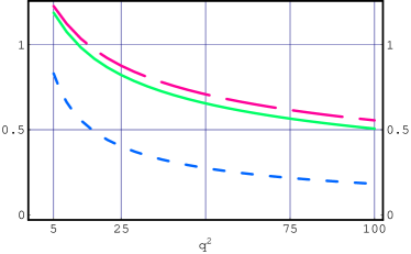
Figure 1: The asymptotic behaviour of the quark form factor is shown as the function of the dimensionless variable $q^{2}=Q^{2}/\Lambda^{2}$, up to terms $O(\ln\ln q^{2})$. The long-dashed (red) presents the contribution of one loop perturbative terms; the solid (green) line represents the total form factor including the instanton induced part, Eq. (53). For comparison, the leading $(\sim\ln q^{2}\ln\ln q^{2})$ perturbative contribution is shown separately—the short-dashed (blue) line.

V Ambiguities of the perturbative result: IR renormalons and analytization of the coupling constant

As it was pointed out in the end of Section II, the perturbative evolution equation (30) possesses an unphysical singularity at the point $\lambda^{2}=1$. Therefore, it is instructive to study the consequences of this feature. It is known that the presence of the Landau pole in the (one-loop) expression for the coupling constant leads to the IR renormalon poles in the Borel plane REN which result in the renormalon-induced power corrections. The latter, being beyond the perturbative evaluations, are treated as a signal of nonperturbative effects which should compensate the ambiguities arising due to these poles. In the present situation, one can expect the corrections proportional to the powers of both scales: $\mu^{2}$ and $\lambda^{2}$. We assume here that the power $\mu^{2}$-terms are too strongly suppressed in large-$q^{2}$ regime and thus can be neglected in the given context, and focus on the power $\lambda^{2}$-corrections. To find them, let us consider the perturbative function $\Delta_{1}(\varepsilon,0,\bar{\mu}^{2}/\lambda^{2})$ in the Eq. (22). The insertion of the fermion bubble 1-chain to the one-loop order expression (19) is equivalent to replacement of the frozen coupling constant $g^{2}$ by the running one $g^{2}\to g^{2}(k^{2})=4\pi\alpha_{s}(k^{2})$ KRREN (for convenience, we work here in Euclidean space):

$$\widetilde{\Delta}_{1}(\varepsilon,0,\bar{\mu}^{2}/\lambda^{2})=-4\pi\bar{\mu}^{2\varepsilon}\int\!{d^{n}k\over(2\pi)^{n}}\alpha_{s}(k^{2}){\hbox{e}^{ikz}\delta(z^{2})\over k^{2}(k^{2}+\lambda^{2})}\ .$$ (54)

Using the integral representation for the one-loop running coupling $\alpha_{s}(k^{2})=\int_{0}^{\infty}\!d\sigma(1/k^{2})^{\sigma b}$, $b=\beta_{0}/4\pi$, we find:

$$\widetilde{\Delta}_{1}(\varepsilon,0,\bar{\mu}^{2}/\lambda^{2})=-{1\over\beta_{0}(1-\varepsilon)}\left(4\pi{\bar{\mu}^{2}\over\lambda^{2}}\right)^{\varepsilon}\int_{0}^{\infty}\!dx\ {\Gamma(1-x-\varepsilon)\Gamma(1+x+\varepsilon)\over(x+\varepsilon)\Gamma(1-\varepsilon)}\left({1\over\lambda^{2}}\right)^{x}\ .$$ (55)

To define properly the integral in r. h. s. of Eq.(55), one needs to specify a prescription to go around the poles, which are at the points $\bar{x}_{n}=n,\ n\in{\mathbb{N}}$. Thus, the result of integration depends on this prescription giving an ambiguity proportional to $\left(1/\lambda^{2}\right)^{n}$ for each pole. Then, the IR renormalons produce the power corrections to the one-loop perturbative result, which we assume to exponentiate with the latter KRREN . Extracting from (55) the UV singular part in vicinity of the origin $x=0$, we divide the integration interval $[0,\infty]$ in two parts: $[0,\delta]$ and $[\delta,\infty]$, where $\delta<1$. This procedure allows us to evaluate separately the ultraviolet and the renormalon-induced pieces. For the ultraviolet piece, we apply the expansion of the integrand in $\Delta_{1}$ in powers of small $x$ and replace the ratio of $\Gamma$-functions by $\exp(-\gamma_{E}\varepsilon)$:

$$\widetilde{\Delta}_{1}^{UV}(\varepsilon,0,\bar{\mu}^{2}/\lambda^{2})=-{1\over\beta_{0}(1-\varepsilon)}\sum_{k,n=0}(-)^{n}{\left(\ln 4\pi-\gamma_{E}+\ln{\bar{\mu}^{2}\over\lambda^{2}}\right)^{k}\over k!\varepsilon^{n-k+1}}\ \int_{0}^{\delta}\!dx\ x^{n}\ \left(1\over\lambda^{2}\right)^{x}\ ,$$ (56)

which after subtraction of the poles in the $\overline{MS}$-scheme becomes:

$$\widetilde{\Delta}_{1}^{UV}(0,\mu^{2}/\lambda^{2})={1\over\beta_{0}(1-\varepsilon)}\ \sum_{n=1}\left(\ln{\mu^{2}\over\lambda^{2}}\right)^{n}{(-)^{n}\over n!}\ \int_{0}^{\delta}\!dxx^{n-1}\left(1\over\lambda^{2}\right)^{x}\ .$$ (57)

In analogy with results of Mikh98 , this expression may be rewritten in a closed form as

$$\widetilde{\Delta}_{1}^{UV}(0,\mu^{2}/\lambda^{2})={1\over\beta_{0}(1-\varepsilon)}\int_{0}^{\delta}\frac{dx}{x}\left[\hbox{e}^{-x\ln\mu^{2}}-\hbox{e}^{-x\ln\lambda^{2}}\right].$$ (58)

Then, using the relation

$${\partial W^{(1)}(q^{2})\over\partial\ln q^{2}}=2C_{F}(1-\varepsilon)\widetilde{\Delta}_{1}^{UV}(0,\mu^{2}/\lambda^{2})\ ,$$ (59)

one finds

$$\left(\mu^{2}{\partial\over\partial\mu^{2}}+\beta(g){\partial\over\partial g}\right){\partial\ln W^{(1)}(q^{2})\over\partial\ln q^{2}}=-{1\over 2}\Gamma_{cusp}^{(1)}(\alpha_{s}(\mu^{2}))\left(1-\exp{\left[-\delta\frac{4\pi}{\beta_{0}\alpha_{s}(\mu^{2})}\right]}\right).$$ (60)

The second exponent in the last equation yields the power suppressed terms $\left(1/q^{2}\right)^{\delta}$ in large-$q^{2}$ regime. In the leading logarithmic approximation (LLA) Eq. (59) is reduced to:

$${\partial W^{(1)}(q^{2})\over\partial\ln q^{2}}=-{2C_{F}\over\beta_{0}}\left(\ln{\ln\mu^{2}\over\ln\lambda^{2}}\right)\ .$$ (61)

The last expression obviously satisfies the perturbative evolution equation (30).

The remaining integral in Eq. (55) over the interval $[\delta,\infty]$ is evaluated at $\varepsilon=0$ since there are no UV singularities. The resulting expression does not depend on the normalization point $\mu$, and thus it is determined by the IR region including nonperturbative effects. It contains the renormalon ambiguities due to different prescriptions in going around the poles $\bar{x}_{n}$ in the Borel plane which yields the power corrections to the quark form factor.

After the substitution $\mu^{2}=q^{2}$ and integration, we find in LLA (for comparison, see Eq. (30)):

$$F_{q}^{ren}(q^{2})=\exp\left[-{2C_{F}\over\beta_{0}}\ln q^{2}\left(\ln\ln q^{2}-1\right)-\ln q^{2}\Phi_{ren}(\lambda^{2})\right]F^{ren}(q_{0}^{2})\ ,$$ (62)

where the function $\Phi_{ren}(\lambda^{2})=\sum_{k=0}\phi_{k}(1/\lambda^{2})^{k}$ accumulates the effects of the IR renormalons. The coefficients $\phi_{k}$ cannot be calculated in perturbation theory and are treated often as “the minimal set” of nonperturbative parameters. It is worth noting that the logarithmic $q^{2}$-dependence of the renormalon induced corrections in the large-$q^{2}$ regime is factorized, and thus the Eq. (62) corresponds to the structure of nonperturbative contributions found in the one-loop evolution equation (30), in a sense of its large-$q^{2}$ behaviour. On the other hand, the IR structures of the renormalon corrections and the instanton induced ones (43) are different. In our point of view, it allows us to separate the true nonperturbative (e.g., instanton induced, but not only) effects from that ones related to ambiguities of the resumed perturbative series.

The latter conclusion can be illustrated by considering the consequences of an analytization of the strong coupling constant SHIR in the perturbative evolution equation. In this approach, the one-loop strong coupling $\alpha_{s}(\mu^{2})$ is replaced by the expression which is analytical at $\mu^{2}=1$ (i.e., at $\Lambda_{QCD}$ in dimensional variables):

$$\alpha_{s}^{AN}(\mu^{2})={4\pi\over\beta_{0}}\left({1\over\ln\mu^{2}}+{1\over 1-\mu^{2}}\right)\ .$$ (63)

The direct substitution of (63) into the evolution equation (15) yields (for brevity, we assume $q_{0}^{2}=\lambda^{2}$):

$$-\left({\beta_{0}\over 2C_{F}}\right)\ln F_{q}^{AN}(q^{2})=$$

$$=\ln q^{2}\ln{\ln q^{2}\over\ln\lambda^{2}}-\ln{q^{2}\over\lambda^{2}}-{3\over 2}\ln{\ln q^{2}\over\ln\lambda^{2}}+$$

$$+\ln q^{2}\left(\ln{q^{2}\over q^{2}-1}+\ln{\lambda^{2}-1\over\lambda^{2}}\right)-{1\over 2}\left(\ln^{2}q^{2}-\ln^{2}\lambda^{2}\right)-$$

$$-\hbox{Li}_{2}(1-q^{2})+\hbox{Li}_{2}(1-\lambda^{2})+{3\over 2}\left(\ln{q^{2}\over q^{2}-1}+\ln{\lambda^{2}-1\over\lambda^{2}}\right)\ .$$ (64)

The functions $\hbox{Li}_{2}$ in the resulting expression accumulate the power corrections of $q^{2}$ as well as IR scale $\lambda^{2}$, but does not exhibit a singularity at $\lambda^{2}=1$. Therefore, it gives no room for IR renormalons ambiguities, at least in the considered approximation. Nevertheless, the power corrections of a nonperturbative origin do contribute to the large-$q^{2}$ behaviour, and the investigation of the correspondence between latter and the instanton corrections calculated in the previous Section would be an interesting task. Note, that the consequences of the analytization of the strong coupling constant in the IR region have been studied earlier in the case of the Sudakov effects in the pion form factor and Drell-Yan cross section in the works STAN .

Another possible way to avoid the Landau pole on the integration path have been developed within the dimensional regularization MAG . In this case, the running coupling reads

$$\alpha_{s}^{DR}(\varepsilon;\mu^{2})={4\pi\varepsilon\over\beta_{0}\left[\left(q^{2}\right)^{\varepsilon}-1\right]}\ ,$$ (65)

and for complex $\varepsilon\ ,\ \hbox{Re}\ \varepsilon<0$ it has the Landau pole at the complex value of $\mu^{2}$, that is this singularity appears to be out of the integration contour. In the limit $\varepsilon\to 0$, the form factor reads MAG (for comparison, see Eq. (30):

$$F_{q}^{DR}(q^{2})=\exp\left[-{2C_{F}\over\beta_{0}}\left({\zeta(2)\over\varepsilon}+\ln\varepsilon\left(\ln q^{2}-{3\over 2}\right)+\ln q^{2}\left(\ln\ln q^{2}-1\right)-{3\over 2}\ln\ln q^{2}\right)+O(\varepsilon,\varepsilon\ln\varepsilon)\right]\ .$$ (66)

This expression also leaves no room for any renormalon induced effects. In the same time, the instanton induced contribution still takes place since they enter into the “integration constant” $W_{np}$ which knows nothing about the analytical properties of the coupling. It should be emphasized that the absence of the IR renormalon induced power corrections obviously does not mean the absence of the power corrections at all. It merely implies that the relations between the ambiguities in the perturbative resummation procedures and the true nonperturbative physics are not so evident and should be studied in more detail.

VI Conclusion

The structure of the nonperturbative corrections to the quark form factor at large momentum transfer was analyzed. In this work, the quarks were assumed to be on-mass shell. In order to model the nonperturbative effects, the quark scattering process was considered in the background of the instanton vacuum. The instanton induced contribution to the electromagnetic quark form factor is calculated in the large momentum transfer regime. It was shown that the instanton induced corrections correspond to the leading term proportional to $\ln q^{2}$. The magnitude of these corrections is determined by the small instanton liquid packing fraction parameter, and they can be treated as finite renormalization of the subleading logarithmic perturbative part (53).

We have to comment that the weak-field limit used in the instanton calculations may deviate from the exact result. Nevertheless, we expect that using of the instanton solution in the singular gauge, that concentrate the field at small distances, leads to the reasonable numerical estimate of the full effect. Thus, the resulting diminishing of the instanton contributions with respect to the perturbative result appears to be reasonable output. It should be emphasized that in the present paper, all the calculations have been performed analytically while the evaluation of the instanton contribution beyond the weak-field approximation requires the numerical analysis, what will be the subject of a separate work. Besides this, the use of the singular gauge for the instanton solution allows one to prove the exponentiation theorem for the Wilson loop in the instanton field DCH1 which permits to express the full instanton contribution as the exponent of the all-order single instanton result (44).

It is also important to note that the results are quite sensitive to the way one makes the integration over instanton sizes finite. For example, if one used the sharp cutoff then the instanton would produce strongly suppressed power corrections like $\propto(1/q)^{\beta_{0}}$. However, we think that the distribution function (45) should be considered as more realistic, since it reflects more properly the structure of the instanton ensemble modeling the QCD vacuum. Indeed, this shape of distribution was recently advocated in SH2 ; DEMM99 (see also DREV and references therein) and supported by the lattice calculations LAT (for comparison, see, however, UKQCD ; SCH2 ).

The instanton induced effects are more interesting for investigation and more important for phenomenology in the hadronic processes which possess two energy scales, such as the total center-of-mass energy $s$ (hard characteristic scale), and the squared momentum transfer $-t$ which is small compared to the latter: $-t<<s$. One of the most interesting examples of such processes is the parton-parton scattering and the soft Pomeron problem Sh ; KKL ; KRP . Another important situations where the nonperturbative (including instanton induced) effects can emerge are the transverse momentum distribution of vector bosons in the Drell-Yan process (see, e.g., KRREN ), and the phenomenon of saturation in deep-inelastic scattering (DIS) at small-x SCHUT . The explicit evaluation of the instanton effects in some of these processes will be the subject of our forthcoming study.

VII Acknowledgements

A major part of the results have been obtained in collaboration with A.E. Dorokhov. I’m grateful to him for numerous fruitful discussions and critical reading of the manuscript. The useful discussions and critical comments of N.I. Kochelev, S.V. Mikhailov and N.G. Stefanis, as well as helpful information and enlightening remarks of B.I. Ermolaev and L. Magnea are thanked. The hospitality and financial support of the Organizers of XXXI ITEP Winter School of Physics is gratefully acknowledged. The work is partially supported by RFBR (Grant nos. 03-02-17291, 02-02-16194, 01-02-16431), Russian Federation President’s Grant no. 1450-2003-2, and INTAS (Grant no. 00-00-366).

References

- (1) Yu. Dokshitzer, D. Dyakonov, S. Troyan, Phys. Reports 58 (1980) 269; A.H. Mueller, Phys. Reports 73 (1981) 237.
- (2) G. Parisi, Phys. Lett. B90 (1980) 295; G. Curci, M. Greco, Phys. Lett. B92 (1980) 175.
- (3) L. Magnea, G. Sterman, Phys. Rev. D42 (1990) 4222; L. Magnea, Nucl. Phys. B593 (2001) 269.
- (4) G. Korchemsky, Phys. Lett. B325 (1994) 459; I. Korchemskaya, Nucl. Phys. B490 (1997) 306.
- (5) R. Petronzio, S. Simula, G. Ricco, Phys. Rev. D67 (2003) 094004.
- (6) V.V. Sudakov, Sov. Phys. JETP 3 (1956) 65; [Zh. Eksp. Teor. Fiz. 30 (1956) 87].
- (7) R. Jackiw, Ann. Phys. (NY) 48 (1968) 292; P.M. Fishbane, J.D. Sullivan, Phys. Rev. D4 (1971) 458.
- (8) J.M. Cornwall, G.Tiktopoulos, Phys. Rev. D13 (1976) 3370; J. Frenkel, J.C. Taylor, Nucl. Phys. B116 (1976) 185; E.C. Poggio, G. Pollack, Phys. Lett. B71 (1977) 135.
- (9) E.A. Kuraev, V.S. Fadin, Yad. Fiz. 27 (1978) 1107.
- (10) B.I. Ermolaev, V.S. Fadin, JETP Lett. 33 (1981) 269; [Pisma Zh. Eksp. Teor. Fiz. 33 (1981) 285]; V.S. Fadin, Sov. J. Nucl. Phys. 37 (1983) 2145; [Yad. Fiz. 37 (1983) 408]; B.I. Ermolaev, V.S. Fadin, L.N. Lipatov, Sov. J. Nucl. Phys. 45 (1987) 508; [Yad. Fiz. 45 (1987) 817].
- (11) V.V. Belokurov, N.I. Usseyukina, Phys. Lett. B94 (1980) 251; H.D. Dahmen, F. Steiner, Z. Phys. C11 (1981) 247.
- (12) A.H. Mueller, Phys. Rev. D20 (1979) 2037; J.C. Collins, Phys. Rev. D22 (1980) 1478.
- (13) A. Sen, Phys. Rev. D24 (1981) 3281.
- (14) G. Korchemsky, Phys. Lett. B217 (1989) 330.
- (15) G. Korchemsky, A. Radyushkin, Sov. J. Nucl. Phys. 45 (1987) 910; G. Korchemsky, A. Radyushkin, Nucl. Phys. B283 (1987) 342.
- (16) G. Korchemsky, Phys. Lett. B220 (1989) 629.
- (17) J.G.M. Gatheral, Phys. Lett. B133 (1983) 90; J. Frenkel, J.C. Taylor, Nucl. Phys. B246 (1984) 231.
- (18) N.G. Stefanis, Nuovo Cim. A83 (1984) 205; R. Jakob, N.G. Stefanis, Annals Phys. 210 (1991) 112; A.I. Karanikas, C.N. Ktorides, N.G. Stefanis, S.M. Wong, Phys. Lett. B455 (1999) 291.
- (19) G.C. Gellas, A.I. Karanikas, C.N. Ktorides, N.G. Stefanis, Phys. Lett. B412 (1997) 95.
- (20) A.I. Karanikas, C.N. Ktorides, N.G. Stefanis, Eur. Phys. J. C26 (2003) 445.
- (21) M. Beneke, Phys. Reports 317 (1999) 1; M. Beneke, V.M. Braun, hep-ph/0010208.
- (22) G. Korchemsky, G. Sterman, Nucl. Phys. B437 (1995) 415; M. Beneke, V.M. Braun, Nucl. Phys. B454 (1995) 253.
- (23) D.V. Shirkov, I.L. Solovtsov, Phys. Rev. Lett. 79 (1997) 1209; D.V. Shirkov, I.L. Solovtsov, hep-ph/9604363.
- (24) F.E. Low, Phys. Rev. D12 (1975) 163.
- (25) S. Nussinov, Phys. Rev. Lett. 34 (1975) 1286.
- (26) P.V. Landshoff, O. Nachtmann, Z. Phys. C35 (1987) 405.
- (27) A. Bassetto, M. Ciafaloni, G. Marchesini, Phys. Reports 100 (1983) 201; O. Nachtmann, Ann. Phys. (N.Y.) 209 (1991) 436.
- (28) E. Shuryak, Nucl. Phys. B203 (1982) 93, 116, 140.
- (29) T. Schäfer, E.V. Shuryak, Rev. Mod. Phys. 70 (1998) 323.
- (30) D. Diakonov, V. Petrov, Nucl. Phys. B245 (1984) 259.
- (31) D. Diakonov, Prog. Part. Nucl. Phys. 51 (2003) 173, hep-ph/0212026.
- (32) H.G. Dosch, Y.A. Simonov, Phys. Lett. B205 (1988) 339; H.G. Dosch, Prog. Part. Nucl. Phys. 33 (1994) 121; O. Nachtmann, hep-ph/9609365.
- (33) B.I. Ermolaev, S.I. Troyan, Nucl. Phys. B590 (2000) 521.
- (34) N.I. Kochelev, Phys. Lett. B565 (2003) 131.
- (35) I. Korchemskaya, G. Korchemsky, Phys. Lett. B287 (1992) 169;
- (36) Yu.M. Makeenko, A.A. Migdal, Phys. Lett. B88 (1979) 135; Nucl. Phys. B188 (1981) 269; A. Polyakov, Gauge Fields and Strings, Harwood, 1987.
- (37) A. Polyakov, Nucl. Phys. B164 (1980) 171; V.S. Dotsenko, S.N. Vergeles, Nucl. Phys. B169 (1980) 527; R.A. Brandt, F. Neri, M.-A. Sato, Phys. Rev. D24 (1981) 879; R.A. Brandt, A. Gocksch, M.A. Sato, F. Neri, Phys. Rev. D26 (1982) 3611.
- (38) A. Ringwald, Nucl. Phys. Proc. Suppl. 121 (2003) 145, hep-ph/0210209.
- (39) A.E. Dorokhov, I.O. Cherednikov, Phys. Rev. D66 (2002) 074009; Eur. Phys. J. A17 (2003) 727.
- (40) A.E. Dorokhov, I.O. Cherednikov, Phys. Rev. D67 (2003) 114017.
- (41) A.E. Dorokhov, hep-ph/0302242
- (42) N. Andrei, D. Gross, Phys. Rev. D18 (1978) 468; L. Baulieu, J. Ellis, M. Gaillard, W. Zakrzewski, Phys. Lett. B77 (1978) 290.
- (43) I.I. Balitsky, Phys. Lett. B273 (1991) 282; V.I. Zakharov, Nucl. Phys. B385 (1992) 452; I.I. Balitsky, V.M. Braun, Phys. Lett. B314 (1993) 237.
- (44) E. Shuryak, I. Zahed, Phys. Rev. D62 (2000) 085014; M. Nowak, E. Shuryak, I. Zahed, Phys. Rev. D64 (2001) 034008.
- (45) D. Kharzeev, Y. Kovchegov, E. Levin, Nucl. Phys. A690 (2001) 621.
- (46) S. Moch, A. Ringwald, F. Schrempp, Nucl. Phys. B507 (1997) 134.
- (47) F. Schrempp, A. Utermann, Phys. Lett. B543 (2002) 197.
- (48) E. Meggiolaro, Phys. Rev. D53 (1996) 3835.
- (49) S.V. Mikhailov, Phys. Lett. B416 (1998) 421.
- (50) G. ’t Hooft, Phys. Rev. D14 (1976) 3432.
- (51) E.V. Shuryak, hep-ph/9909458.
- (52) A.E. Dorokhov, S.V. Esaibegyan, S.V. Mikhailov, Phys. Rev. D56 (1997) 4062; A.E. Dorokhov, S.V. Esaibegyan, A. E. Maximov, S.V. Mikhailov, Eur. Phys. J. C13 (2000) 331, hep-ph/9903450.
- (53) A. Hasenfratz, C. Nieter, Phys. Lett. B439 (1998) 366.
- (54) T.R. Morris, D.A. Ross, C.T. Sachrajda, Nucl. Phys. B255 (1985) 115.
- (55) A.I. Karanikas, N.G. Stefanis, Phys. Lett. B504 (2001) 225; N.G. Stefanis, W. Schroers, H.C. Kim, Eur. Phys. J.C18 (2000) 137.
- (56) D.A. Smith, M.J. Teper [UKQCD collaboration], Phys. Rev. D58 (1998) 014505.
- (57) F. Schrempp, J. Phys. G28 (2002) 915.
- (58) F. Schrempp, A. Utermann, hep-ph/0301177.