Supernovæ and Light Neutralinos: SN1987A Bounds on Supersymmetry Revisited

Abstract

For non-universal gaugino masses, collider experiments do not provide any lower bound on the mass of the lightest neutralino. We review the supersymmetric parameter space which leads to light neutralinos, $M_{{\tilde{\chi}}}\,\,\raisebox{-3.44444pt}{$\stackrel{{\scriptstyle\textstyle<}}{{\sim}}$ }{\cal O}(1\,{\rm GeV})$, and find that such neutralinos are almost pure bino. In light of this, we examine the neutralino lower mass bound obtained from supernova 1987A (SN1987A). We consider the production of binos in both electron-positron annihilation and nucleon-nucleon binostrahlung. For electron-positron annihilation, we take into account the radial and temporal dependence of the temperature and degeneracy of the supernova core. We also separately consider the Raffelt criterion and show that the two lead to consistent results. For the case of bino production in $NN$ collisions, we use the Raffelt criterion and incorporate recent advances in the understanding of the strong-interaction part of the calculation in order to estimate the impact of bino radiation on the SN1987A neutrino signal. Considering these two bino production channels allows us to determine separate and combined limits on the neutralino mass as a function of the selectron and squark masses. For $M_{{\tilde{\chi}}}\sim 100\,{\rm MeV}$ values of the selectron mass between 300 and 900 GeV are inconsistent with the supernova neutrino signal. On the other hand, in contrast to previous works, we find that SN1987A provides almost no bound on the squark masses: only a small window of values around 300 GeV can be excluded, and even then this window closes once $M_{{\tilde{\chi}}}\,\,\raisebox{-3.44444pt}{$\stackrel{{\scriptstyle\textstyle>}}{{\sim}}$ }20\,{\rm MeV}$.

1 Introduction

If the supersymmetry-breaking, electroweak, gaugino masses fulfill the grand-unified mass relation:

$$M_{1}=\frac{5}{3}\tan^{2}\!\theta_{w}M_{2},$$ (1)

then, because LEP chargino and neutralino-pair-production searches set a lower bound on $M_{2}$, there is a concomitant lower bound on $M_{1}$. These constraints on the mass matrix result (for the case of conserved R-parity) in a limit on the mass of the lightest neutralino, ${{\tilde{\chi}}}$ [1]:

$$M_{{{\tilde{\chi}}}}\geq 46\,{\rm GeV}.$$ (2)

However, Eq. (1) is not an inescapable consequence of unification. For example, unification might occur through a string theory without a simple gauge group [2]. Refs. [3, 4] showed that if the assumption (1) is dropped and $M_{1}$ and $M_{2}$ are considered as independent free parameters then there is currently no lower experimental bound on the neutralino mass from collider experiments  . In light of this situation, here we reconsider the bounds on neutralino properties which can be determined from supernova 1987A (SN1987A) [5, 6, 7, 8].

The basic idea is that in a supernova, neutralinos with masses of order the supernova core temperature, $T_{c}={\cal O}(30\,{\rm MeV})$, can be produced in large numbers via electron-positron annihilation [5, 7] and nucleon-nucleon ($NN$) “neutralinostrahlung” [6]:

$$e^{+}+e^{-} \longrightarrow {{\tilde{\chi}}}+{{\tilde{\chi}}}\,,$$ (3)

$$N+N \longrightarrow N+N+{{\tilde{\chi}}}+{{\tilde{\chi}}}\,.$$ (4)

Once produced, the neutralinos have a mean-free-path, $\lambda_{{\tilde{\chi}}}$, in the supernova core which is determined via the cross sections for the processes [5, 6, 7]:

$${{\tilde{\chi}}}+e \longrightarrow {{\tilde{\chi}}}+e\,,$$ (5)

$${{\tilde{\chi}}}+N \longrightarrow {{\tilde{\chi}}}+N\,,$$ (6)

as well as the electron and nucleon densities. If $\lambda_{{\tilde{\chi}}}$ is of order the core size, $R_{c}={\cal O}(10\,{\rm km})$, or larger, the neutralinos escape freely and thus cool the supernova rapidly. As the supernova temperature drops, the neutrino scattering cross section also drops and the neutrinos are no longer trapped, thereby further hastening the cooling of the supernova. Thus neutralino cooling could significantly shorten the supernova neutrino signal [9], in disagreement with the observation from SN1987A by the Kamiokande and IMB collaborations [10, 11]. However, if the neutralinos have masses $M_{{\tilde{\chi}}}$ much greater than the supernova core temperature $T_{c}$ then their production is Boltzmann-factor suppressed and they affect the cooling negligibly, independent of $\lambda_{{\tilde{\chi}}}$. Demanding that $M_{{\tilde{\chi}}}$ be large enough that neutralino-cooling does not markedly alter the neutrino signal—particularly its time-structure—allows us to set a lower limit on the neutralino mass. As we discuss in detail below, this limit depends on the squark and selectron masses which determine the relevant neutralino cross sections for the production processes (3) and (4), as well as those for the scattering processes (5) and (6).

A full treatment of this physics requires the implementation of the neutralinos into the supernova simulation code. This is well beyond the scope of this paper. Instead we invoke two different analytic criteria to estimate whether neutralino emission will affect the detected neutrino signal significantly. The first test we consider is to require the integrated supernova energy emitted through the neutralino channel to be less than

$$E_{{\tilde{\chi}}}^{\rm max}=10^{52}\,{\rm erg}\,,$$ (7)

i.e. much smaller than the energy emitted by all neutrino species: $E_{\nu}\approx 3.0\times 10^{53}\,{\rm erg}$ [12]. The exact number we choose here is somewhat arbitrary–not least since it is subject to our ignorance of the total energy released in SN1987A. We will discuss the dependence of our neutralino mass bounds on $E_{{\tilde{\chi}}}^{\rm max}$ below.

Detailed supernova simulations with axions suggest that another way to place bounds on these energy-loss mechanisms is the “Raffelt criterion” [12]. This states that “exotic” cooling processes, such as those considered here, will not alter the neutrino signal observably, provided that their emissivity, $\dot{\cal E}$, obeys:

$$\dot{\cal E}<10^{19}~{}{\rm ergs/g/s}.$$ (8)

If their emissivity is larger than this they will remove sufficient energy from the explosion to invalidate the current understanding of a Type-II supernova neutrino signal. With this simple criterion the results of the detailed simulations in Refs. [13, 14]—where the exotic cooling mechanisms considered were axions [13] and KK-graviton emission [14]—can be reproduced. These detailed simulations also show that the feature of the SN1987A neutrino pulse which is most affected by the presence of alternative cooling mechanisms is the temporal distribution. Losing $10^{52}$ ergs to neutralinos during the first $\sim$ 1 second after bounce, as in our first criterion (7), might not greatly affect neutrino temporal and spectral features. But, at later times, the loss of just a fraction of this energy could have a dramatic impact—by ending the period of diffusive neutrino cooling much earlier than would otherwise be the case. In this paper, we examine the impact of the process (3) using first Eq. (7) and then the Raffelt criterion, Eq. (8), and compare the results. We find good agreement between the two.

Neither of these criteria are particularly suitable in the case that neutralinos have a small mean-free-path, $\lambda_{{\tilde{\chi}}}\,\,\raisebox{-3.44444pt}{$\stackrel{{\scriptstyle\textstyle<}}{{\sim}}$ }{\cal O}(R_{c})$, since the neutralinos’ contribution to the proto-neutron star cooling is then diffusive, rather than radiative. The treatment of this “trapped” regime is beyond the scope of this study. In Sec. 6 we make an estimate of the conditions for trapping and then refer the reader to the literature for bounds on SUSY parameters under these conditions [5, 6, 7]. In this work, we focus on estimating the emitted energy in neutralinos, assuming they are weakly coupled to matter, and then applying the criteria (7) and (8).

Previous authors [5, 6, 7] considered the case of a stable neutralino and were thus restricted to the mass regions [15] :

$$M_{{\tilde{\chi}}}\,\,\raisebox{-3.44444pt}{$\stackrel{{\scriptstyle\textstyle<}}{{\sim}}$ }100~{}{\rm eV}\,\qquad{\rm or}\qquad M_{{\tilde{\chi}}}\,\,\raisebox{-3.44444pt}{$\stackrel{{\scriptstyle\textstyle>}}{{\sim}}$ }500\,{\rm MeV}\,,$$ (9)

in order to avoid an over-closed universe. The heavier neutralinos, $M_{{\tilde{\chi}}}>500\,{\rm MeV}$, are irrelevant for supernovæ and thus Refs. [5, 6, 7] focused on a massless neutralino. In this work we consider the range:

$$0\leq M_{{\tilde{\chi}}}\leq 200\,{\rm MeV}\,.$$ (10)

We avoid over-closure of the universe by allowing for the possibility of a small amount of R-parity violation [20, 21], and thus assume that the neutralinos, although stable on the time scale of the supernova and collider experiments, are not stable on cosmological timescales. For such neutralinos, which we call “quasi-stable”, the mass restriction (9) does not apply .

To summarize: in this work we consider a general lower mass bound on quasi-stable neutralinos as a function of the squark and selectron masses. We assume the bounds from the relic density are avoided through small R-parity violating couplings. This is similar in outlook to Ref. [8] where, in light of the Karmen time anomaly [24], the impact on SN1987A of a neutralino with the specific mass ($M_{{\tilde{\chi}}}=34\,{\rm MeV}$) was examined. We extend this work to a general neutralino. We also differ from previous work in the following more technical points

1. Throughout we consider a bino neutralino instead of a photino, since in Refs. [3, 4] it was shown that a light neutralino, $M_{{\tilde{\chi}}}\,\,\raisebox{-3.44444pt}{$\stackrel{{\scriptstyle\textstyle<}}{{\sim}}$ }5\,{\rm GeV}$, must be dominantly bino in order to be consistent with LEP results. This leads to a substantially weaker effective coupling to nucleons and thus to weaker bounds on the supersymmetric-particle masses.

2. For the case of electron-positron annihilation and the criterion Eq (7), we consider the radial and temporal dependence of the temperature and the degeneracy in the core [25]. This gives a more realistic estimate of this contribution. It also gives a stricter bound than some previous work [6] since the temperature in the outermost region of the star ($r\approx\frac{9}{10}R_{c}$), where most of the neutralinos coming from annihilation are produced, is somewhat higher than the temperature considered by, for instance, Ref. [7]. However, it gives a weaker bound than in the earlier work by Ellis et al., Ref. [6], where a significantly higher core temperature was chosen. Since all emissivities vary rapidly with temperature this results in a marked difference in the bounds on the supersymmetric-particle masses.

3. The calculation of the $NN\rightarrow NN{{\tilde{\chi}}}{{\tilde{\chi}}}$ emissivity by Ellis et al. was based on the computation of the rate for the related neutrinostrahlung process: $NN\rightarrow NN\nu{\bar{\nu}}$ [6]. For this Ellis et al. used the pioneering calculation of Friman and Maxwell, Ref. [26]. A recent model-independent treatment of $NN$ dynamics in the production of axial radiation—e.g. by reactions such as $NN\rightarrow NN\nu\bar{\nu}$ or $NN\rightarrow NN{{\tilde{\chi}}}{{\tilde{\chi}}}$—suggests that Ref. [26] overestimates supernova emissivities by about a factor of four [27, 28, 29]. This loosens the bound previously obtained from SN1987A on the relevant supersymmetric-particle masses.

4. Since previous authors only considered very light neutralinos, $M_{{\tilde{\chi}}}$ was neglected in computing the total neutralino emissivity. We calculate the full $M_{{\tilde{\chi}}}$-dependence of $\dot{\cal E}_{{\tilde{\chi}}}$. In particular, for $M_{{\tilde{\chi}}}\,\,\raisebox{-3.44444pt}{$\stackrel{{\scriptstyle\textstyle>}}{{\sim}}$ }T_{c}$ the mass dependence is very strong. Indeed, ultimately it is exactly this strong mass dependence which we use to derive a bound on $M_{{\tilde{\chi}}}$.

5. We also combine the emissivities from both electron-positron annihilation and nucleon-nucleon neutralinostrahlung to get a bound on supersymmetric-particle masses from both sources of neutralino radiation.

The outline of the paper is as follows. In Sec. 2, we discuss the possibility of a light neutralino in the MSSM. In Sec. 3, we determine the bounds which can be found from electron-positron annihilation. This allows us to exclude certain regions of the joint parameter space of selectron and neutralino masses. In Sec. 4, we determine the effective neutralino-nucleon coupling. In Sec. 5, we use this to compute the general bound obtained from $NN\rightarrow NN{{\tilde{\chi}}}{{\tilde{\chi}}}$ as a function of $M_{{\tilde{\chi}}}$ and $M_{\tilde{q}}$. This analysis can be applied to the production of any particle pair which is axially coupled to nucleons. In Sec. 6 we discuss the effect that neutralino trapping due to matter and/or gravitational interactions has on these bounds. Finally, in Sec. 7 we combine the results for $e^{+}e^{-}\rightarrow{{\tilde{\chi}}}{{\tilde{\chi}}}$ and $NN\rightarrow NN{{\tilde{\chi}}}{{\tilde{\chi}}}$ in order to get overall information on the regions of MSSM parameter-space which are excluded, and offer our conclusions.

2 A Light Neutralino in the MSSM

Before we discuss in detail the bounds we obtain from SN1987A on a light neutralino, we consider whether such a neutralino is consistent within the MSSM and with existing collider data. In Ref. [3] it was shown that there are no laboratory bounds on a neutralino with mass $M_{{\tilde{\chi}}}=34\,{\rm MeV}$, provided it is dominantly bino—mainly because a bino neutralino does not couple to the $Z^{0}$-boson at tree-level. For a neutralino with mass $M_{{\tilde{\chi}}}<{\cal O}(200\,{\rm MeV})$—which we consider here—none of the bounds in Refs. [3, 4] depend sensitively on the mass. We thus expect such a neutralino to be consistent with all terrestrial data .

We have gone beyond Refs. [3, 4], and looked in more detail at where in the MSSM parameter space a neutralino with $M_{{\tilde{\chi}}}\leq 200$ MeV can be obtained. We have found new parameter regions which are shown in Fig. 1. Note particularly that for a fixed value of $M_{1}$ there can be more than one value of $M_{2}$ leading to a specific $M_{{\tilde{\chi}}}$. It is also clear that, as was pointed out in Ref. [31], neutralino zero modes are possible. These are the downward spikes in Fig. 1. There are in fact extensive regions in the $M_{1}-M_{2}$ parameter space where a light neutralino can be obtained. However, if we take into account the lower mass bound on the chargino from LEP2 ($M_{2}>120\,{\rm GeV}$ ), we see that for $\tan\beta=10$ and $\mu=300\,{\rm GeV}$ a light neutralino is only obtained for the specific range $1\,{\rm GeV}<M_{1}<1.5\,{\rm GeV}$. (These parameter values will be shifted by the one-loop radiative corrections to the gaugino masses.) This involves a relative fine-tuning of $10^{-2}$ between $M_{1}$ and $M_{2}$. While this is perhaps æsthetically displeasing, it is by no means forbidden.

In this parameter range, the neutralino is more than 98% bino. In the following we shall thus work with a pure bino. Our only free supersymmetric parameters are then $M_{{\tilde{\chi}}}$ and the selectron and squark masses.

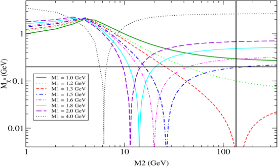
Figure 1: The neutralino mass as a function of $M_{2}$ for various values of $M_{1}$ and with $\tan\beta=10$, $\mu=300\,{\rm GeV}$. The downward spikes correspond to true zeros of the neutralino mass. The bold horizontal line indicates the value $M_{{\tilde{\chi}}}=200\,{\rm MeV}$, below which we consider in this paper. To the right of the bold vertical line at about $M_{2}=120\,{\rm GeV}$ the chargino mass satisfies the lower mass bound from LEP2.

3 Electron-Positron Annihilation to Neutralinos

We first discuss the case of free-streaming neutralinos. We defer the issue of trapped neutralinos to Sec. 6, where we consider their scattering off electrons and nucleons in the supernova environment, as well as gravitational trapping.

3.1 Emissivity for Free Streaming Neutralinos

The neutralinos are produced via electron-positron annihilation

$$e^{+}(p_{1})+e^{-}(p_{2})\rightarrow{{\tilde{\chi}}}(k_{1})+{{\tilde{\chi}}}(k_{2})\,,$$ (11)

where we have indicated the four-momenta of the particles. The dominant process proceeds via $t$- and $u$-channel selectron exchange. The energy thus emitted by the supernova per unit time and unit volume is the emissivity

$$\dot{\cal E}(M_{{\tilde{\chi}}},T_{c},\eta)\equiv\frac{d{\cal E}}{dt}=\int\frac{d^{3}p_{1}d^{3}p_{2}}{(2\pi)^{6}}\,f_{1}f_{2}\,(E_{1}+E_{2})\;|\Delta{\bf v}|\,\sigma(e^{+}+e^{-}\rightarrow{{\tilde{\chi}}}+{{\tilde{\chi}}})\,.$$ (12)

Here $E_{1}+E_{2}=E_{3}+E_{4}$ is the combined energy of the emitted neutralinos. The Fermi-Dirac distributions are given by

$$f_{i}=\frac{1}{e^{(E_{i}\pm\mu_{i})/T_{c}}+1}\;,$$ (13)

where $\mu_{i}$ is the chemical potential and $T_{c}$ the temperature in the supernova. In the following, we shall write $\eta\equiv\mu/T_{c}$ for the degeneracy of the electrons. We have neglected the Pauli blocking of the final state neutralinos: $(1-f_{3})(1-f_{4})$. In Eq. (12), $\sigma(e^{+}+e^{-}\rightarrow{{\tilde{\chi}}}+{{\tilde{\chi}}})$ is the (free-space) cross section for the process (11) and $|\Delta{\bf v}|$ is the absolute value of the relative Møller velocity

$${v}_{\rm{M\!{\not\,o}l}}=\sqrt{(\mathbf{v}_{1}-\mathbf{v}_{2})^{2}-(\mathbf{v}_{1}\times\mathbf{v}_{2})^{2}}\;\stackrel{{\scriptstyle{v_{i}\rightarrow 1}}}{{\longrightarrow}}\;(1-\cos\theta)\;.$$ (14)

(${\bf v}_{i}$ are the velocities of the incoming electron and positron and $\theta$ is the angle between them.) In the case where the selectron masses are degenerate, $M_{{\tilde{e}}_{L}}=M_{{\tilde{e}}_{R}}=M_{\tilde{e}}$ the cross section is given by

$$\sigma(e^{+}+e^{-}\rightarrow{{\tilde{\chi}}}+{{\tilde{\chi}}})=\frac{17\pi\alpha^{2}s}{24\cos^{4}\theta_{w}M_{\tilde{e}}^{4}}\left(1-\frac{4M_{{\tilde{\chi}}}^{2}}{s}\right)^{3/2}\!\!\!,$$ (15)

where we have used $m_{e}^{2}\ll s\ll M_{\tilde{e}}^{2}$. Here $\alpha$ is the fine structure constant, $\theta_{w}$ is the electroweak mixing angle and $s$ is the center-of-mass energy squared. Replacing the bino-coupling by the photino coupling this agrees with Ref. [32].

The emissivity in Eq. (12) is a function of the neutralino mass via the cross section (15). It is a function of the supernova temperature and $\eta$ via the Fermi-Dirac distributions (13).

3.2 Total Emitted Energy

In order to determine the total energy emitted in the neutralino channel we must integrate the emissivity over the time, $t_{0}$, during which neutralinos are emitted and over the volume of the supernova core

$$E_{{\tilde{\chi}}}(M_{{\tilde{\chi}}})=\int_{0}^{t_{0}}\!dt\int\!d^{3}r\;\dot{\cal E}(M_{{\tilde{\chi}}},T_{c}({\bf r},t),\eta({\bf r},t))\equiv\int_{0}^{t_{0}}\!dt\;P(M_{{\tilde{\chi}}},t)\,.$$ (16)

When performing these integrations care must be taken since the temperature and the degeneracy depend on the radius and on the time. We use the temperature distribution given in Fig. 1 of Ref. [25]. There the temperature is shown as a function of the enclosed baryon mass. In Fig. 5 of Ref. [25] we see that for $t\geq 250$ ms the density is constant. This makes the conversion of $d^{3}r$ to $dM$ straightforward. Here we adopt a core radius of $R_{c}=13$ km and a mass of $M_{\rm SN}=1.4\,M_{\odot}$ and obtain

$$\rho\approx 3\times 10^{14}~{}{\rm g}/{\rm cm^{3}}.$$ (17)

(Throughout we assume radial symmetry [25].)

The time $t=0$ of Ref. [25] corresponds to the time when the incoming shock wave stops and bounces outwards again. The boundary conditions at this time are not well known [33]. However, the exact shape of the initial conditions has little effect on the subsequent evolution and after 0.5 s the distributions are reliable. For the first second we have used the $t=0.5\,$s distributions of Ref. [25]. For longer time scales we have used the subsequent radial distributions for $T_{c}({\bf r},t)$ and $\eta({\bf r},t)$. However, as we will show below, most of the energy is emitted during the first second after the bounce and so ultimately we will use $t_{0}=1$ second in (16) to derive our neutralino mass bounds. This means that we are demanding that the prompt neutralino pulse in the first second does not have a total energy greater than the bound (7) . We discuss below how the neutralino-mass bound depends on the value chosen for $t_{0}$.

3.3 Results

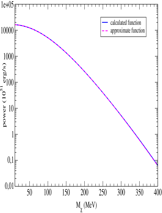
Figure 2: Neutralino power $P_{{\tilde{\chi}}}(M_{{\tilde{\chi}}},t)$ for $t=0.5$ seconds as a function of the neutralino mass, $M_{{\tilde{\chi}}}$, with the selectron mass $M_{{\tilde{e}}}=200\,{\rm GeV}$. The solid curve shows our numerical computation while the dashed curve represents the fit Eq. (18). The two curves are almost indistinguishable.

Before presenting the total emitted energy, we consider the power radiated in the neutralino channel. In Fig. 2, we show as the solid curve the power of the neutralino emission at $t=0.5\;$s as a function of the neutralino mass, $P(M_{{\tilde{\chi}}},0.5~{}{\rm s})$. We have fixed the selectron mass to $M_{{\tilde{e}}}=200\,{\rm GeV}$. According to Eq. (15), the power scales as $M_{{\tilde{e}}}^{-4}$. A good fit to the solid curve throughout most of the neutralino mass range is given by

$$P(x)=C\left(\frac{200\,{\rm GeV}}{M_{\tilde{e}}}\right)^{4}\exp(a_{4}x^{4}+a_{3}x^{3}+a_{2}x^{2}+a_{1}x)\,,\qquad x\equiv\frac{M_{{\tilde{\chi}}}}{{\rm MeV}}\,,$$ (18)

where the constants are given by

$$a_{1} = 1.71\times 10^{-3}\,,\qquad\;\,a_{2}\,=\,-1.58\times 10^{-4}$$

$$a_{3} = 2.695\times 10^{-7}\,,\qquad a_{4}\,=-1.99\times 10^{-10}\,\,,\qquad C=1.6318\times 10^{55}\;{\rm erg/s}.$$ (19)

The numerical fit in Eq. (18) is shown as the dashed curve in Fig. 2. Throughout the mass range considered it agrees to better than 1% and the two curves are almost indistinguishable.

When using the Raffelt criterion it is also convenient to have a parameterization for the emissivity

$${\dot{\cal E}}(M_{{\tilde{\chi}}})=D\left(\frac{200\,{\rm GeV}}{M_{\tilde{e}}}\right)^{4}\exp(b_{4}x^{4}+b_{3}x^{3}+b_{2}x^{2}+b_{1}x)\,,\qquad x\equiv\frac{M_{{\tilde{\chi}}}}{{\rm MeV}}\,,$$ (20)

and the constants are given by

$$b_{1} = 4.75\times 10^{-4}\,,\qquad b_{2}\,=\,-2.25\times 10^{-4}$$

$$b_{3} = 4.66\times 10^{-7}\,,\qquad b_{4}\,=\,-4.02\times 10^{-10}\,,\qquad D=9.0125\times 10^{21}\;{\rm erg/g/s}.$$ (21)

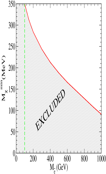
Figure 3: The dependence of the neutralino lower mass bound on the selectron mass. Here we chose $E_{{\tilde{\chi}}}^{\rm max}=10^{52}\,$erg and $t_{0}=1\,$s. The green-dashed line indicates the lower bound on the selectron mass from LEP2. Beyond $M_{\tilde{e}}=1$ TeV the exclusion curve drops rapidly.

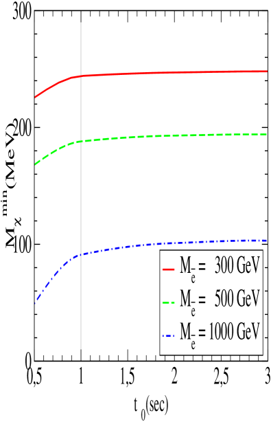
Figure 4: The minimum allowed value of $M_{{\tilde{\chi}}}$, $M_{{\tilde{\chi}}}^{\rm min}$, as a function of the time over which we integrate, $t_{0}$. The curves correspond to three different values of the selectron mass: $M_{\tilde{e}}=300,\,500,\,1000\,{\rm GeV}$. Here $E_{{\tilde{\chi}}}^{\rm max}=10^{52}\,$erg and the neutralino is pure bino. Our choice of $t_{0}=1$ second is indicated by the grey vertical line.

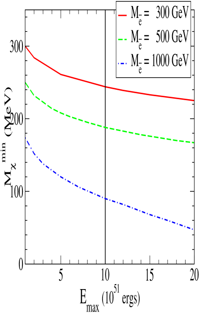
Figure 5: The neutralino mass bound as a function of $E_{{\tilde{\chi}}}^{\rm max}$ for three different values of the selectron mass: $M_{\tilde{e}}=300,\,500,\,1000\,{\rm GeV}$. Here $t_{0}=1\,$s and the neutralino is again pure bino. Our choice of Eq. (7) is represented by the black vertical line.

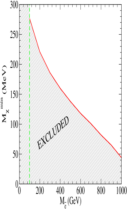
Figure 6: The neutralino lower mass bound as a function of the selectron mass $M_{\tilde{e}}$, when the Raffelt criterion is applied to the emissivity for electron-positron annihilation to neutralinos. The vertical line indicates the lower bound on the selectron mass from LEP2 [35].

Once we have computed $E_{{\tilde{\chi}}}(M_{{\tilde{\chi}}})$ we can determine a smallest permitted neutralino mass by requiring the emitted energy to be below $E_{{\tilde{\chi}}}^{\rm max}$ of Eq. (7). If we choose $E_{{\tilde{\chi}}}^{\rm max}=10^{52}\,$erg, $t_{0}=1\,$s and the neutralino to be pure bino then for $M_{\tilde{e}}=300\,{\rm GeV}$ we have:

$$M_{{\tilde{\chi}}}^{\rm min}=243\,{\rm MeV},$$ (22)

while for $M_{\tilde{e}}=1$ TeV we find $M_{{\tilde{\chi}}}^{\rm min}=90\,{\rm MeV}$. For a massless neutralino to be allowed we require $M_{\tilde{e}}\geq 1275\,{\rm GeV}$.

The value of $M_{{\tilde{\chi}}}^{\rm min}$ is shown for a wide range of selectron masses in Fig. 3. Note that values of $M_{{\tilde{\chi}}}$ below the solid (red) line are forbidden, as are values of $M_{\tilde{e}}$ to the left of the solid line, since in either case the total energy produced by the process (11) in the first one second will be larger than $E_{{\tilde{\chi}}}^{\rm max}$. The lower selectron mass bound from LEP2 [35]:

$$M_{{\tilde{e}}}\;>\;99.6\,{\rm GeV}\,,$$ (23)

is also indicated by the vertical dashed (green) line in the figure.

How sensitive are these results to the choice $t_{0}=1$ second? We made this choice because we expect most of the neutralino power to be emitted in a burst during the early, hottest, part of the supernova. This is indeed the case. If we integrate the power out further, thereby increasing $t_{0}$, and again apply the criterion (7), we obtain the bounds shown in Fig. 4. Once $t_{0}>1$ second the bound is essentially independent of $t_{0}$.

As discussed above, the exact value chosen for $E_{{\tilde{\chi}}}^{\rm max}$—$10^{52}$ ergs—is somewhat arbitrary. In Fig. 5 we show the dependence of the lowest-allowed $M_{{\tilde{\chi}}}$ on the choice of $E_{{\tilde{\chi}}}^{\rm max}$. This is done for several values of the selectron mass. Note that if $E_{{\tilde{\chi}}}^{\rm max}$ is decreased (increased) by a factor of two then $M_{{\tilde{\chi}}}^{\rm min}$ becomes at most 25% larger (40% smaller).

Thus, the main dependence of the neutralino mass bound is on the selectron mass, which sets the effective electron-neutralino coupling strength. In addition, it is important to note that most of the neutralino production from electron-positron annihilation occurs in the outermost 10% of the star ($\frac{9}{10}R_{c}\,\,\raisebox{-3.44444pt}{$\stackrel{{\scriptstyle\textstyle<}}{{\sim}}$ }r\,\,\raisebox{-3.44444pt}{$\stackrel{{\scriptstyle\textstyle<}}{{\sim}}$ }R_{c}$). Looking at the profiles used for density and temperature during the first one second [25] the reason for this becomes apparent. At early times, this outer region has the highest temperature, and, more importantly, the lowest electron degeneracy, $\eta$. Since the rate of the process (11) is suppressed by factors of $e^{-\eta}$, the smaller values of $\eta$ near the surface of the star mean that the majority of neutralinos are produced there. This will prove critical when we look at the effect of neutralino trapping on our bounds in Sec. 6.

3.4 Raffelt Criterion for $e^{+}e^{-}\rightarrow{{\tilde{\chi}}}{{\tilde{\chi}}}$

Although we have used the best supernova input available for radial temperature and density profiles, and have argued that our results are not especially sensitive to our choices for $E_{{\tilde{\chi}}}^{\rm max}$ and $t_{0}$, we would like to check the bounds on $M_{{\tilde{\chi}}}$ as a function of $M_{\tilde{e}}$ that resulted from our modeling of the supernova. To this end we now turn to the Raffelt criterion (8). This is an estimate of what would happen were the neutralinos implemented in a full simulation of SN1987A. It is a test that is local in space and time—unlike the integral measure (7).

The one parameter we are free to choose in applying (8) is the temperature at which $\dot{\cal E}_{{\tilde{\chi}}}$ is to be computed. Previous work suggests $T_{c}=30\,{\rm MeV}$ is a reasonable choice [13, 14, 36]. Computing the emissivity due to $e^{+}e^{-}\rightarrow{{\tilde{\chi}}}{{\tilde{\chi}}}$ at this temperature, and at a density of $3\times 10^{14}~{}{\rm g}/{\rm cm^{3}}$, produces the constraint on neutralino and selectron masses shown in Fig. 6. The solid (red) line indicates the neutralino and selectron masses for which the emissivity of the process (11) is exactly $10^{19}$ ergs/g/s. Neutralino masses below the solid (red) line, and selectron masses to the left of it, are forbidden. According to the criterion (8), if the supersymmetric particles had such masses the time-structure of the observed SN1987A neutrino pulse would have been noticeably different.

Note that the bound obtained with the Raffelt criterion is a little less stringent than that obtained from (7) and depicted in Fig. 3. The two criteria would be in agreement if we chose $E_{{\tilde{\chi}}}^{\rm max}$ to be roughly a factor of two larger. Alternatively, if in the Raffelt criterion we chose the supernova core temperature to be $T_{c}=34\,{\rm MeV}$, we would also obtain agreement between the two approaches.

Thus the qualitative agreement between these “global” and “local” criteria gives us confidence in the computationally-simpler Raffelt criterion—confidence that is supported by detailed simulations of the impact of axions [13] and KK-gravitons [14] on the SN1987A neutrino signal. From now on we will use the Raffelt criterion to assess the impact of neutralinos on the cooling of SN1987A.

4 Neutralino-Nucleon Interactions

We now turn our attention to the “binostrahlung” process (4). We wish to evaluate the emissivity due to this reaction. To do this, in Sec. 5 we compute the Feynman graphs shown in Fig. 7. This gives the amplitude for the process (4) to leading-order in the soft-radiation approximation.

Figure 7: Two diagrams contributing to neutralinostrahlung from the nucleon-nucleon system. Time flows from left to right. The nucleons are denoted by double lines. The (yellow) oval indicates the nucleon-nucleon interaction. The black circle indicates the effective neutralino-nucleon coupling which we compute in Sec. 4. Two diagrams which are the same, except that the neutralinos are radiated from the bottom lines, are not shown.

These two diagrams, together with their partners under $1\leftrightarrow 2$ interchange, give the dominant result for binostrahlung in the limit that the total neutralino energy $\omega\rightarrow 0$, since they are the only graphs which diverge ($\sim 1/\omega$) in that limit. Indeed, were the radiation a single photon, rather than a ${{\tilde{\chi}}}{{\tilde{\chi}}}$ pair, the graphs in Fig. 7 would yield the leading-order Low energy theorem for $NN\rightarrow NN\gamma$ [27, 37, 38]. In order to evaluate them we need to know two amplitudes: the nucleon-nucleon interaction, denoted by a (yellow) oval in Fig. 7, and the effective neutralino-nucleon interaction, represented by a large black dot in Fig. 7.

In the soft-radiation limit the intermediate-state nucleon line in Fig. 7 is almost on-shell. Thus, as we explain in Sec. 5 and Appendix A below, to leading order in the soft-radiation expansion, the nucleon-nucleon interaction occurs on-mass-shell. In consequence, it can be reconstructed from $NN$ scattering data, giving a model-independent result for this piece of input to the diagrams in Fig. 7.

In this section, we focus on the other piece of input to these diagrams: the neutralino-nucleon coupling. We will show that in the limit of long-wavelength (i.e. soft) neutralinos this coupling is expressible in terms of the spin content of the nucleon, $\Delta q$. We evaluate the ${{\tilde{\chi}}}n$ coupling using two different sets of results for $\Delta u$, $\Delta d$, and $\Delta s$: the predictions of the non-relativistic quark model (NRQM), and those of the quark-parton picture at leading order in $\alpha_{s}$ (LO-QPM). The neutralino-neutron coupling turns out to be very different in these two cases, and this difference has a considerable impact on our final predictions for the emissivity due to $nn$ binostrahlung. We believe this gives an estimarte of the range of permitted values.

4.1 The Bino-Quark Four-Fermion Effective Lagrangian

The Lagrangian for a pure bino-neutralino coupling to a quark and a squark is given by [39]:

$${\cal L}_{q\tilde{q}{{\tilde{\chi}}}} = -\,\frac{e}{\sqrt{2}\cos\theta_{w}}\sum_{q}\left[Y_{q_{R}}\,({\bar{q}}_{R}P_{L}{{{\tilde{\chi}}}})\,{\tilde{q}}_{R}+Y_{q_{L}}\,{\tilde{q}}^{*}_{L}({\bar{{\tilde{\chi}}}}\,P_{L}q)\,\right],$$ (24)

where $e$ denotes the electric charge. The sum runs in our case over the quarks $q=u,d,s$ and ${\tilde{q}}_{L,R}$ denotes the corresponding left- or right-handed squark. The hypercharges $Y_{q_{R}}$ for the right-handed singlet quarks are given by: $Y_{u_{R}}=-\frac{4}{3}$, and $Y_{d_{R}}=Y_{s_{R}}=\frac{2}{3}$. For the left-handed quarks $Y_{q_{L}}=\frac{1}{3}$. For each term in the Lagrangian we obtain two crossed Feynman diagrams contributing to neutralino pair emission from a nucleon, as shown in Fig. 8. In the following we shall assume that the squark masses are degenerate:

$$M_{\tilde{q}}\equiv M_{{\tilde{d}}_{L}}=M_{{\tilde{d}}_{R}}=M_{{\tilde{u}}_{L}}=M_{{\tilde{u}}_{R}}\,.$$ (25)

Since the momentum transfer in the neutralinostrahlung in our case satisfies $Q^{2}\ll M_{\tilde{q}}^{2}$, we can obtain an effective four-fermion operator for the $qq{{\tilde{\chi}}}{{\tilde{\chi}}}$ interaction for a pure bino [40]:

$${\cal L}_{qq{{\tilde{\chi}}}{{\tilde{\chi}}}} = \frac{e^{2}}{8\cos^{2}\theta_{w}\,M^{2}_{\tilde{q}}}({\bar{{\tilde{\chi}}}}\gamma^{\mu}\gamma^{5}{{\tilde{\chi}}})\sum_{q}\left[Y_{q_{L}}^{2}\,({\bar{q}}\gamma_{\mu}P_{L}q)\,-Y_{q_{R}}^{2}\,({\bar{q}}\gamma_{\mu}P_{R}q)\,\right].$$ (26)

Here we have performed a Fierz transformation in order to separate the neutralino current from the quark current. The vector current for the neutralinos vanishes since they are Majorana fermions.

Figure 8: The two diagrams contributing to neutralinostrahlung from a nucleon. The (green) oval denotes the nucleon bound state. The horizontal lines are the partons with ${\rm\bf q=u,d,s}$. The virtual squark ${\rm\bf\tilde{q}}$ can be either left- or right-handed.

The quark current can be split into a vector and an axial-vector part:

$${\cal L}_{qq{{\tilde{\chi}}}{{\tilde{\chi}}}}=-\frac{e^{2}}{16M_{\tilde{q}}^{2}\cos^{2}\theta_{W}}\,(\bar{{{\tilde{\chi}}}}\gamma^{\mu}\gamma_{5}{{\tilde{\chi}}})\sum_{q}[W_{q}^{2}\;\bar{q}\gamma_{\mu}q+X_{q}^{2}\;\bar{q}\gamma_{\mu}\gamma_{5}q]\,,$$ (27)

with the effective charges ($W_{q}^{2}\equiv Y_{q_{R}}^{2}-Y_{q_{L}}^{2}$, $X_{q}^{2}\equiv Y_{q_{R}}^{2}+Y_{q_{L}}^{2}$):

$$W_{u}^{2}=\;\frac{15}{9}\,; W_{d}^{2}=\;W_{s}^{2}\;=\;\frac{1}{3}\,,$$ (28)

$$X_{u}^{2}=\;\frac{17}{9}\,; \,X_{d}^{2}=\;X_{s}^{2}\;=\;\frac{5}{9}\,.$$ (29)

4.2 Nucleon Matrix Elements

The neutralino coupling to nucleons can be calculated by taking matrix elements of the interaction in Eq. (27) between nucleon states. In the limit that $Q^{2}\ll\Lambda_{QCD}^{2}$ this interaction energy can be rewritten in terms of an axial neutralino current coupling to quark vector and axial-vector current matrix elements:

$$V_{{{\tilde{\chi}}}{{\tilde{\chi}}}nn}=\frac{e^{2}}{16M_{\tilde{q}}^{2}\cos^{2}\theta_{W}}\,[\,\bar{{{\tilde{\chi}}}}\gamma^{\mu}\gamma_{5}{{\tilde{\chi}}}]\,\sum_{q}(W_{q}^{2}V^{(q)}_{\mu}+X_{q}^{2}A^{(q)}_{\mu})\,,$$ (30)

with:

$$V^{(q)}_{\mu} = \langle n|\int d^{3}x\,\bar{q}(x)\gamma_{\mu}q(x)|n\rangle\,,$$ (31)

$$A^{(q)}_{\mu} = \langle n|\int d^{3}x\,\bar{q}(x)\gamma_{\mu}\gamma_{5}q(x)|n\rangle\,.$$ (32)

These quark-current matrix elements simplify to:

$$V^{(q)}_{\mu}=\langle n|\frac{{\rm P}_{\mu}}{M_{n}}|n\rangle N_{q}^{(n)}\,,$$ (33)

$$A^{(q)}_{\mu}=\langle n|\Sigma_{\mu}|n\rangle\,\Delta q^{(n)},$$ (34)

where ${\rm P}_{\mu}$ and $M_{n}$ are the momentum and the mass of the neutron, $N_{q}^{(n)}$ is the number of valence quarks of type $q$ in the neutron, $\Sigma_{\mu}$ is twice the Pauli-Lubanski spin vector, and $\Delta q^{(n)}$ is the average contribution of quarks of type $q$ to the total neutron spin.

For a neutron at rest, the only component of $V^{(q)}_{\mu}$ which is non-zero is the zeroth one, while the four-vector $\Sigma_{\mu}$ has only non-zero spatial components. Thus we arrive at an interaction energy:

$$V_{{{\tilde{\chi}}}{{\tilde{\chi}}}nn}=\frac{e^{2}}{16M_{\tilde{q}}^{2}\cos^{2}\theta_{W}}\left[\bar{{{\tilde{\chi}}}}\gamma^{0}\gamma_{5}{{\tilde{\chi}}}\left(\sum_{q}W_{q}^{2}N_{q}^{(n)}\right)n^{\dagger}n-\bar{{{\tilde{\chi}}}}\vec{\gamma}\gamma_{5}{{\tilde{\chi}}}\cdot(n^{\dagger}\vec{\sigma}_{n}n)\left(\sum_{q}X_{q}^{2}\,\Delta q^{(n)}\right)\right]\,,$$ (35)

with $\vec{\sigma}_{n}$ the three-vector of the neutron Pauli spin matrices. Corrections to Eq. (35) are suppressed by powers of ${\bf P}_{n}/M_{n}$ and/or powers of $QR_{n}$, with $R_{n}$ the neutron’s size. This allows us to write an effective four-fermion Lagrangian for the interaction of neutralinos with non-relativistic neutrons:

$${\cal L}_{{{\tilde{\chi}}}{{\tilde{\chi}}}nn}=-\frac{G_{SUSY}}{2\sqrt{2}}a^{\mu}\left[n^{\dagger}\left(c_{\rm v}^{\chi}\delta_{\mu,0}-c_{\rm a}^{\chi}\delta_{\mu,i}\sigma_{i}\right)n\right]\,,$$ (36)

with the axial-vector neutralino current:

$$a^{\mu}\equiv\bar{{{\tilde{\chi}}}}\gamma^{\mu}\gamma_{5}{{\tilde{\chi}}}\,,$$ (37)

and the effective couplings:

$$\qquad\qquad G_{SUSY}\equiv\frac{e^{2}}{4\sqrt{2}\cos^{2}\theta_{W}M_{\tilde{q}}^{2}}\,,$$ (38)

$$c_{\rm v}^{\chi}=\frac{19}{9}\,;\qquad c_{\rm a}^{\chi}=\frac{17}{9}\,\Delta d+\frac{5}{9}(\,\Delta u+\,\Delta s).$$ (39)

(In (39) we have used the conventional definitions of the $\Delta q$’s and isospin.)

The two diagrams in Fig. 7 enter with opposite signs in the computation of the amplitude for the radiative process. Thus, as we discuss further in Sec. 5, to leading order in $1/M_{n}$ the vector-current interaction does not contribute to the neutralinostrahlung emissivity. Hereafter we disregard its contribution in order to get the lowest-order result for the binostrahlung emissivity in the soft-radiation approximation. It is worth bearing in mind though that $1/M_{n}$ corrections, as well as effects due to non-zero proton fraction, could render vector-current radiation quite significant in binostrahlung.

Note that, in general, the vector current dominates neutralino-neutron scattering, which we will examine in Sec. 6.

This leaves us with the task of estimating $\Delta u$, $\Delta d$, and $\Delta s$. We consider only two out of a plethora of approaches:

1. Employ the non-relativistic quark model (NRQM). In this case:

   $$\Delta u=\frac{4}{3};\qquad\Delta d=-\frac{1}{3};\qquad\Delta s=0,$$ (40)

   giving:

   $$c_{\rm a}^{\chi}=\frac{1}{9}\,.$$ (41)

2. Employ the leading order quark parton model (LO-QPM) [41]. This obeys the constraint $\Delta u-\Delta d=g_{A}$, and does not fare too badly with respect to the constraint from the $F/D$ ratio extracted from hyperon decays [42]:

   $$\Delta u+\Delta d-2\Delta s\approx 0.682\,.$$ (42)

   The values from Ref. [41] are:

   $$\Delta u=0.78\pm 0.03\,;\qquad\Delta d=-0.48\pm 0.03\,;\qquad\Delta s=-0.14\pm 0.03\,.$$ (43)

   These values rely on the extraction of the flavour-singlet matrix element from the zeroth moment of the protons $g_{1}$ structure function, and its subsequent evolution to low-$Q^{2}$. This evolution is perhaps questionable, since below $Q^{2}\sim 1\,{\rm GeV}^{2}$ it becomes non-perturbative. Nevertheless, the values (43) give:

   $$c_{\rm a}^{\chi}=-0.55\pm 0.06\,,$$ (44)

   a result five times as large as the NRQM one, and of opposite sign.

4.3 Ratio of Neutralino and Neutrino Processes

We now follow Ref. [6], and take the ratio of the coupling $c_{a}^{\chi}$ to the corresponding neutrino coupling, in an attempt to eliminate some of the uncertainties in the computation.

The effective Lagrangian for the neutrino case is [26, 27, 43]:

$${\cal L}_{\nu\nu nn}=-\frac{G_{F}}{2\sqrt{2}}\;l^{\mu}\;[n^{\dagger}(c_{\rm v}^{\nu}\delta_{\mu,0}-c_{\rm a}^{\nu}\delta_{\mu,i}\sigma_{i})n]\,,$$ (45)

with the leptonic current:

$$l^{\mu}\equiv\bar{\nu}\gamma^{\mu}(1-\gamma_{5})\nu\,.$$ (46)

Here we will drop the vector-current piece, since it does not contribute to $nn\rightarrow nn\nu\bar{\nu}$. Meanwhile, arguments analogous to those of the previous subsection yield:

$$c_{\rm a}^{\nu}=-[\Delta u-\Delta d+\Delta s].$$ (47)

In the non-relativistic quark model we have:

$$c_{\rm a}^{\nu}=-\frac{5}{3}\,,$$ (48)

while using the values for the $\Delta q\,$’s from the quark-parton model in Eq. (43) we find:

$$c_{\rm a}^{\nu}=-1.12\pm 0.05\,.$$ (49)

The latter value is about 33% lower than in the NRQM: a significantly smaller discrepancy than in the neutralino case.

Therefore for our chosen evaluation procedures the ratio of neutralino to neutrino axial coupling constants is:

$$\frac{c_{\rm a}^{\chi}}{c_{\rm a}^{\nu}}=\left\{\begin{array}[]{ll}-\frac{1}{15}&\quad\mbox{NRQM}\,,\\ &\\ 0.49\pm 0.08&\quad\mbox{LO-QPM}\,.\end{array}\right.$$ (50)

In order to use the the effective Lagrangian (45) to compute the neutrino emissivity due to the reaction $nn\rightarrow nn\nu\bar{\nu}$, we require the spin-summed matrix element for $nn\rightarrow nn\nu\bar{\nu}$ [26, 27, 43]:

$$\sum_{\nu~{}{\rm spin}}|{\cal M}|^{2}=\frac{G_{F}^{2}(c_{\rm a}^{\nu})^{2}}{8}{\rm Tr}(l_{i}l_{j})\left(\frac{16}{\omega^{2}}\right){\cal H}_{ij}\,.$$ (51)

Here ${\cal H}_{ij}$ is the hadronic tensor, which corresponds to two insertions of the neutron spin in the hadronic (in this case $nn$) state. The evaluation of this quantity will be discussed in Sec. 5, but note that we have already used the fact that only its spatial components are non-zero in the non-relativistic limit. (Here and below we denote spatial indices by Roman letters.) Also, for later convenience, we have removed a factor of $1/\omega^{2}$, to take care of the leading behavior of $|{\cal M}|^{2}$ in the soft-radiation limit, as well as a factor of $16$, to account for identical particles and the fact that the neutrinos couple to both nucleons. ($\omega$ is the total emitted neutralino energy.) The sum over hadronic states in ${\cal H}_{ij}$ will then only include states permitted by the Pauli principle.

Meanwhile, ${\rm Tr}(l_{i}l_{j})$ are the space-space components of the neutrino tensor:

$$\ell^{\mu\nu} \equiv {\rm Tr}[\not\!k_{1}\gamma_{\mu}(1-\gamma_{5})\not\!k_{2}\gamma_{\nu}(1-\gamma_{5})]\,,$$ (52)

$$= 8\left[k_{1}^{\mu}k_{2}^{\nu}+k_{2}^{\mu}k_{1}^{\nu}-g^{\mu\nu}k_{1}\cdot k_{2}+i\epsilon_{\alpha\mu\beta\nu}k_{1}^{\alpha}k_{2}^{\beta}\right],$$ (53)

in agreement with Friman and Maxwell [26] ($k_{1,2}$ are the outgoing neutrino momenta).

Now, in order to compute the spin-squared matrix element for $nn\rightarrow nn{{\tilde{\chi}}}{{\tilde{\chi}}}$ we proceed by analogy with this neutrino calculation. The spin-summed matrix element for neutralinostrahlung which is integrated to yield the neutralino emissivity due to the process (4) can be written as:

$$\sum_{{{\tilde{\chi}}}~{}{\rm spin}}|{\cal M}|^{2}=\frac{G_{SUSY}^{2}{c_{\rm a}^{\chi}}^{2}}{8}{\rm Tr}(a_{i}a_{j})\left(\frac{16}{\omega^{2}}\right){\cal H}_{ij}\,.$$ (54)

Crucially, the hadronic tensor here is the same as the one in Eq. (51), since neutralino-pair production is also induced by two insertions of the neutron-spin operator in the hadronic system.

We now compute the neutralino tensor ${\rm Tr}(a_{i}a_{j})$. It is to be understood as the space-space piece of the four-tensor:

$${\cal N}^{\mu\nu} \equiv Tr[(\not\!k_{1}+M_{{\tilde{\chi}}})\gamma^{\mu}\gamma_{5}(\not\!k_{2}-M_{{\tilde{\chi}}})\gamma^{\nu}\gamma_{5}]\,,$$ (55)

$$= 4\left[k_{1}^{\mu}k_{2}^{\nu}+k_{1}^{\nu}k_{2}^{\mu}-(k_{1}\cdot k_{2}-M_{{\tilde{\chi}}}^{2})g^{\mu\nu}\right],$$ (56)

where $k_{1}$ and $k_{2}$ are now the outgoing neutralino four-momenta.

In order to compare the neutralino and neutrino computations it is convenient to define $\alpha_{{\tilde{\chi}}}$ to be the ratio of neutralino to neutrino spin-summed matrix elements, with the ratio taken in the limit $M_{{\tilde{\chi}}}=0$. Then:

$$\alpha_{{\tilde{\chi}}}\equiv\left(\frac{G_{SUSY}\;c_{\rm a}^{\chi}}{G_{F}\;c_{\rm a}^{\nu}}\right)^{2}\frac{{\cal N}_{ij}{\cal H}_{ij}}{\ell_{ij}{\cal H}_{ij}},$$ (57)

where ${\cal H}_{ij}$ is the hadronic spin response in both cases.

In the computation that follows in Sec. 5, we assume that the nucleons are in thermal equilibrium, with a common temperature $T_{c}$. Thus the nucleon kinetic energies are of order $T_{c}$, and their momenta are of order $\sqrt{M_{n}T_{c}}$. The centre-of-mass energy of the reaction (4) is therefore also thermally distributed around $2T_{c}$. This means that neutralinos are produced with a common “temperature” $\sim T_{c}$. For $M_{{\tilde{\chi}}}\,\,\raisebox{-3.44444pt}{$\stackrel{{\scriptstyle\textstyle<}}{{\sim}}$ }50\,{\rm MeV}$, the neutralinos are then relativistic and have momenta of order $T_{c}\ll\sqrt{M_{n}T_{c}}$. Consequently, to leading order in $\sqrt{T_{c}/M_{n}}$ we can ignore the recoil of the hadronic system when the neutralinos are emitted, and ${\cal H}_{\mu\nu}$ will then be independent of ${\bf k}_{1}$ and ${\bf k}_{2}$. This allows us to perform the integral over these variables and obtain an “angle-averaged” neutralino tensor:

$${\overline{\cal N}}_{\mu\nu}\equiv\int\frac{d\Omega_{1}}{4\pi}\int\frac{d\Omega_{2}}{4\pi}{\cal N}_{\mu\nu}\,,$$ (58)

and analogously for the neutrino case. For the space-space components—which are all that are relevant here—this gives:

$$\overline{\cal N}_{ij} = \delta_{ij}4(\omega_{1}\omega_{2}-M_{{\tilde{\chi}}}^{2})\,;$$

$$\overline{\ell}_{ij} = \delta_{ij}8\omega_{1}\omega_{2}\,,$$ (59)

where $\omega_{1,2}$ are the energies of the two emitted neutrinos/neutralinos.

In any observable—including emissivities—in which the outgoing neutr(al)inos are not detected we can use these “angle-averaged” leptonic tensors in the evaluation of the spin-summed matrix element—provided, of course, that we truly are in the kinematic regime where recoil of the hadronic system can be neglected. Calculating $\alpha_{{\tilde{\chi}}}$ using the tensors (59) we get:

$$\alpha_{{\tilde{\chi}}} = \frac{1}{2}\left(\frac{G_{SUSY}\;c_{\rm a}^{\chi}}{G_{F}\;c_{\rm a}^{\nu}}\right)^{2}$$ (60)

$$= \frac{\sin^{4}\theta_{W}}{2}\left(\frac{M_{Z}}{M_{\tilde{q}}}\right)^{4}\left(\frac{c_{\rm a}^{\chi}}{c_{\rm a}^{\nu}}\right)^{2}.$$ (61)

Note that the hadronic tensor has canceled, so this ratio is independent of the model of the nuclear medium that is adopted. Note also that all of the nucleon-model dependence is now isolated in the last factor. Finally, Eq. (61) gives:

$$\alpha_{{\tilde{\chi}}}\approx\sin^{4}\theta_{W}\left(\frac{M_{Z}}{M_{\tilde{q}}}\right)^{4}\times\left\{\begin{array}[]{ll}\frac{1}{450}&\quad\mbox{NRQM}\,,\\ &\\ \frac{1}{8}&\quad\mbox{LO-QPM}\,,\end{array}\right.$$ (62)

where we have written $0.49\approx\frac{1}{2}$. $\alpha_{{\tilde{\chi}}}$ is more than fifty times larger in the LO-QPM than in the NRQM.

5 Emission from a Neutron Gas

We are now ready to compute the emissivity due to neutron-neutron “neutralinostrahlung”, the process (4). (For simplicity we will restrict ourselves to pure neutron matter. The generalization to arbitrary proton fraction is straightforward, if somewhat cumbersome.) We shall derive a general emissivity, which is valid for any particle-pair which couples axially to the nucleons. We then demand that this emissivity is not larger than the Raffelt bound (8), and so set bounds on $\alpha_{{\tilde{\chi}}}$. At the end of this section we use the results of Sec. 4 to translate our bound on $\alpha_{{\tilde{\chi}}}$ into a bound on the squark mass.

It was recently shown that, for soft radiation, the neutrino emissivity due to $nn\rightarrow nn\nu\bar{\nu}$ can be directly related to the on-shell nucleon-nucleon data [27]. For $M_{{\tilde{\chi}}}\,\,\raisebox{-3.44444pt}{$\stackrel{{\scriptstyle\textstyle<}}{{\sim}}$ }50\,{\rm MeV}$, this “soft-radiation approximation” also provides a model-independent way to compute the emissivity due to neutralinostrahlung. On the other hand, for neutralino masses of order 100 MeV or more the radiation cannot be regarded as soft, since $M_{{\tilde{\chi}}}\sim m_{\pi}$, and the pion plays an important role in $NN$ scattering and in bremsstrahlung dynamics. However, even for large (from a nuclear physics point of view) neutralino masses we still regard the method presented here as a useful way to get an order of magnitude estimate of the emissivity due to $nn\rightarrow nn{{\tilde{\chi}}}{{\tilde{\chi}}}$. As will be demonstrated below, this emissivity depends sensitively on $M_{{\tilde{\chi}}}$ through the Boltzmann factors and so, even if our estimate of the matrix element is off by an order of magnitude, the neutralino-mass bound changes by only about 30%.

The emissivity for the radiation of neutralinos from an interacting neutron gas is given by

$$\dot{\cal E} = \int d\omega\int\left[\prod_{i=1,2}\frac{d^{3}p_{i}\,d^{3}p_{i}^{\prime}}{(2\pi)^{6}}\right](2\pi)^{4}\delta^{(4)}(p_{1}+p_{2}-p_{1}^{\prime}-p_{2}^{\prime}-k)$$ (63)

$$\ \qquad\qquad\qquad\qquad\qquad\times\ S\cdot f(E_{1})f(E_{2})(1-f(E_{1}^{\prime}))(1-f(E_{2}^{\prime}))\frac{dE}{d\omega}\ ,$$

where $S=1/8$ is the symmetry factor taking into account that the initial and final nucleon pairs, as well as the neutralinos are identical. $p_{1},\,p_{2}$ are the incoming and $p_{1}^{\prime},\,p_{2}^{\prime}$ are the outgoing neutron four-momenta. $f(E)$ is the Fermi-Dirac distribution function (13). The energy per unit frequency interval for a particular two-neutron phase-space element is given by:

$$\frac{dE}{d\omega}=\int\frac{d^{3}k_{1}}{(2\pi)^{3}2\omega_{1}}\frac{d^{3}k_{2}}{(2\pi)^{3}2\omega_{2}}\,\omega\,\delta(\omega-\omega_{1}-\omega_{2})\delta^{(3)}(k-k_{1}-k_{2})|{\cal M}|^{2}.$$ (64)

$\omega$ and ${\bf k}$ are the total energy and three-momentum of the neutralino pair, and $k_{1,2}$ are the three-momenta of the neutralinos. ${\cal M}$ is the matrix element for the process $nn\rightarrow nn{{\tilde{\chi}}}{{\tilde{\chi}}}$.

To proceed, we now use the decomposition of $|{\cal M}|^{2}$ into a hadronic tensor and a neutralino tensor as given in Eq. (54). Introducing this into Eq. (64) and using the angle-averaged expression of Eq. (58) for the neutralino tensor, we derive

$$\frac{dE}{d\omega}=\alpha_{{\tilde{\chi}}}G_{F}^{2}{c_{\rm a}^{\nu}}^{2}\frac{1}{\pi^{4}}\int\,d\omega_{1}d\omega_{2}\,\delta(\omega-\omega_{1}-\omega_{2})\,\frac{k_{1}k_{2}}{\omega}\,(\omega_{1}\omega_{2}-M_{{\tilde{\chi}}}^{2}){\cal H}_{ii}\,,$$ (65)

Here $\alpha_{{\tilde{\chi}}},\,G_{F},\,c_{\rm a}^{\nu}$ are as defined in Sec. 4. We will now set bounds on $\alpha_{{\tilde{\chi}}}$ which apply to any axially-coupled light-particle-pairs emitted from the neutron gas. We then translate to bounds on the squark mass $M_{\tilde{q}}$ using Eq. (62).

5.1 Evaluating the Hadronic Tensor

In Section 4, we saw that when calculating the neutr(al)ino emissivity only the space-space diagonal elements of the hadronic tensor are required. To leading order in the soft-radiation approximation, and provided many-body effects are not large, only the diagrams shown in Fig. 7 contribute to ${\cal H}_{ii}$. The tensor can then be expressed in terms of the commutator of the production operator with the $NN$ scattering matrix $T_{NN}$ [27]. According to ${\cal L}_{{{\tilde{\chi}}}{{\tilde{\chi}}}nn}$ of Eq. (36), in the non-relativistic limit only two operator structures govern the ${{\tilde{\chi}}}{{\tilde{\chi}}}$ pair’s coupling: the unit operator and the spin operator. The commutator of the unit operator with $T_{NN}$ vanishes, and therefore the vector current in Eq. (36) does not contribute to $nn\rightarrow nn{{\tilde{\chi}}}{{\tilde{\chi}}}$. Thus, at leading order the only structure which contributes to ${\cal H}_{ij}$ is the two-nucleon spin operator, $S_{i}$. For a given two-nucleon state of total energy $E$, we find that the relevant, diagonal, components of ${\cal H}_{ij}$ are:

$${\cal H}_{ii}(E)=\sum_{m_{s},m_{s}^{\prime}}|\langle 1\,m_{s}^{\prime},\,{\bf p}^{\prime}|\,[S_{i},T_{NN}]\,|{\bf p},\,1\,m_{s}\rangle|^{2}\,,$$ (66)

where $|{\bf p},\,1\,m_{s}\rangle$ is a two-nucleon state of total spin 1, total spin projection $m_{s}$, and relative momentum ${\bf p}$. Here, because the binos radiated in Fig. 7 are soft, the initial and final $nn$ relative momenta obey:

$${\bf p}^{2}={\bf p}^{\prime 2}=ME\,.$$ (67)

The key point here is that the $NN$ matrix elements in Eq. (66) are on-shell, and so can be obtained from nucleon-nucleon scattering data. So, to leading order in the soft-radiation approximation, there is a direct connection between this data and the neutralino emissivity $d{\cal E}/dt$: a connection given by Eqs. (66), (65) and (63).

To further simplify Eq. (63), spherical symmetry and energy-momentum conservation can be exploited, thereby eliminating nine of the eighteen integrals. We define total, initial relative, and final relative momenta ${\bf P}$, ${\bf p}$, and ${\bf p}^{\prime}$, respectively, and also move to dimensionless variables [44]:

$$\tau^{2}=\frac{{\bf P}^{2}}{8MT_{c}}\,,\qquad\delta=\frac{{\bf p}^{2}-{\bf p}^{\prime}\,{}^{2}}{2MT_{c}}\,,\qquad\sigma=\frac{{\bf p}^{2}+{\bf p}^{\prime 2}}{2MT_{c}}\,,$$ (68)

and

$$\eta_{n}=\frac{\mu}{T_{c}}\,,\qquad\hat{M}_{{\tilde{\chi}}}=\frac{M_{{\tilde{\chi}}}}{T_{c}}\,,$$ (69)

where $T_{c}$ is the temperature of the neutron gas in the supernova. At large temperatures, the angular dependence of the Fermi functions becomes weak—in the non-degenerate limit the angular dependence disappears completely. We have checked that at the temperatures we are studying replacing the product of Fermi functions by their angular average is justified. These angular integrals can be performed analytically [44]:

$$\int_{-1}^{1}\,d\gamma\,f(E_{1})f(E_{2})=\frac{e^{-\xi^{2}}}{\tau(\delta+\sigma)\sinh(\xi^{2})}\ln\left(\frac{\cosh\left[\frac{1}{2}\left\{\xi^{2}+\tau(\delta+\sigma)\right\}\right]}{\cosh\left[\frac{1}{2}\left\{\xi^{2}-\tau(\delta+\sigma)\right\}\right]}\right)\ ,$$ (70)

where $\xi^{2}=\frac{1}{4}(\delta+\sigma)^{2}+\tau^{2}-\eta_{n}$. Doing the angular integrals this way necessitates the introduction of the angle-averaged hadronic tensor:

$$\overline{\cal H}_{ii}=\int\,\frac{d\hat{p}\,d\hat{p}^{\prime}}{16\pi^{2}}\,{\cal H}_{ii}\ .$$ (71)

The replacement ${\cal H}_{ii}\longrightarrow\overline{\cal H}_{ii}$ is not only a good approximation, it is a useful one, since the integrals in Eq. (71) be carried out analytically, when the $NN$ $T$–matrix is given in partial wave form. The procedure used to construct $\overline{\cal H}_{ii}$ from a given set of $NN$ phase shifts is sketched in Appendix A. The results that follow were generated using the VPI phase-shift analysis in that construction [45].

5.2 Emissivity

We now return to the computation of the emissivity Eq. (63). Doing the angular integrals as described leaves us with a four-dimensional integral which we decompose as

$$\dot{\cal E}=\alpha_{{\tilde{\chi}}}\,\frac{G_{F}^{2}c_{A}^{2}}{8(2\pi)^{11}}\,(2MT_{c})^{9/2}M_{{\tilde{\chi}}}^{4}\int_{\hat{M}_{{\tilde{\chi}}}}^{\infty}d\delta\,e^{-\delta}h(\delta/\hat{M}_{{\tilde{\chi}}})\int_{\delta}^{\infty}d\sigma\,{\cal F}(\delta,\sigma,\eta_{n})\,\bar{\cal H}_{ii}(T_{c}\,\sigma)\,,$$ (72)

where

$$h(y)=\frac{1}{y}(y-1)^{3}\left[(y^{2}+1)I_{0}(y)-(y-1)^{2}I_{2}(y)\right],$$ (73)

with

$$I_{k}(y)=\int_{-1}^{1}\,dx\,x^{k}\sqrt{(1-x^{2})(Y^{2}(y)-x^{2})}\,,$$ (74)

and $Y(y)\equiv(y+1)/(y-1)$. The result of the angular integration of the Fermi functions is

$${\cal F}(\delta,\sigma,\eta_{n})=\int_{0}^{\infty}d\tau\,{\cal R}\left(\sqrt{\frac{1}{2}(\sigma+\delta)},\tau,\eta_{n}\right){\cal R}\left(\sqrt{\frac{1}{2}(\sigma-\delta)},\tau,\eta_{n}\right),$$ (75)

where

$${\cal R}(a,\tau,\eta_{n})=\frac{1}{\sinh(a^{2}+\tau^{2}-\eta_{n})}\ln\left(\frac{\cosh\left(\frac{1}{2}((\tau+a)^{2}-\eta_{n})\right)}{\cosh\left(\frac{1}{2}((\tau-a)^{2}-\eta_{n})\right)}\right).$$ (76)

The functions $I_{k}(y)$ can be evaluated to very high accuracy if we replace the second factor in the square root by its Taylor expansion up to third order in $(x/Y)^{2}$. Formally one would expect this approximation to work for $Y\gg 1$ only. However, even for $Y=1$ both $I_{2}$ as well as $I_{0}$ turn out to be within 5% of the exact result. The remaining 3 integrals are evaluated numerically using the Gauss-Legendre method. The computation was performed for nuclear matter density and $T_{c}=30\,{\rm MeV}$. The result of the numerical integration is shown as the solid line in Fig. 9 for $\alpha_{{\tilde{\chi}}}=2.5\times 10^{-4}$.

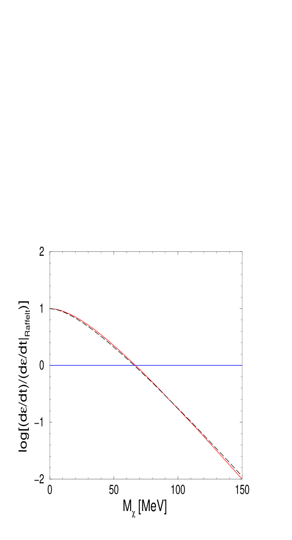
Figure 9: Neutralino emissivity in units of $10^{19}$ ergs/g/s as a function of the neutralino mass $M_{{\tilde{\chi}}}$. The red solid line shows the full result for $\alpha_{{\tilde{\chi}}}=10\,\alpha_{{\tilde{\chi}}}^{\rm crit}$, whereas the black dashed line shows the fit according to Eq. (77). The horizontal blue solid line shows the emissivity $10^{19}$ ergs/g/s that is used when the Raffelt criterion is applied.

The numerical result is well fit by:

$$\dot{\cal E}=4\alpha_{{\tilde{\chi}}}\ (1+2\hat{M}_{{\tilde{\chi}}}+0.55\hat{M}_{{\tilde{\chi}}}^{2})\ e^{-2\hat{M}_{{\tilde{\chi}}}}\ \times\ 10^{23}\ \mbox{[ergs/g/s]},$$ (77)

where $\hat{M}_{{\tilde{\chi}}}\equiv M_{{\tilde{\chi}}}/T_{c}$ as defined in Eq. (69). The fit is good for $M_{{\tilde{\chi}}}\,\,\raisebox{-3.44444pt}{$\stackrel{{\scriptstyle\textstyle<}}{{\sim}}$ }200\,{\rm MeV}$. Our result represented in the form (77) allows us to directly derive a neutralino mass bound for any given coupling strength $\alpha_{{\tilde{\chi}}}$ using the Raffelt criterion (8). Alternatively, we can think of defining a function $\alpha_{{\tilde{\chi}}}^{\rm crit}(M_{{\tilde{\chi}}})$ from Eq. (77): the coupling at which the Raffelt criterion is exactly met for a given neutralino mass $M_{{\tilde{\chi}}}$.

By setting $\hat{M}_{{\tilde{\chi}}}=0$ in Eq. (77) above, i.e. a massless neutralino, we obtain the minimal coupling $\alpha_{{\tilde{\chi}}}^{\rm crit}(0)$, for which we can set a bound. Using Eq. (8) we obtain

$$\alpha_{{\tilde{\chi}}}^{\rm crit}(0)=2.5\times 10^{-5}.$$ (78)

For $M_{{\tilde{\chi}}}=T_{c}=30\,{\rm MeV}$, $\alpha_{{\tilde{\chi}}}^{\rm crit}(M_{{\tilde{\chi}}})$ increases to $5.2\times 10^{-5}$. For $M_{{\tilde{\chi}}}>T_{c}$, the minimum $\alpha_{{\tilde{\chi}}}$ we are sensitive to changes rapidly with the neutralino mass due to the exponential dependence seen in Eq. (77). Using the Raffelt criterion we can exclude a region in the $\alpha_{{\tilde{\chi}}}$–$M_{{\tilde{\chi}}}$ plane which is to the right of the curve defined by the function $\alpha_{{\tilde{\chi}}}^{\rm crit}(M_{{\tilde{\chi}}})$; this region is shown in Fig. 10.

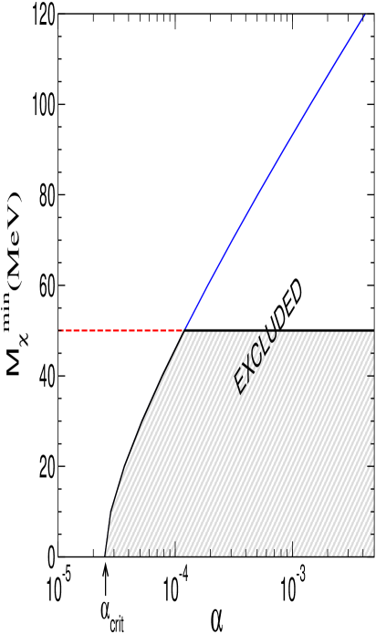
Figure 10: The region of the $\alpha_{{\tilde{\chi}}}$-$M_{{\tilde{\chi}}}$(MeV) plane that is excluded by our soft-radiation calculation, when applying the Raffelt criterion (at $T_{c}=30\,{\rm MeV}$) is indicated by the grey shading. The blue solid line is the curve that defines the values of $\alpha_{{\tilde{\chi}}}$ and $M_{{\tilde{\chi}}}$ which produce a neutralino emissivity of exactly $10^{19}$ ergs/g/s. The horizontal (red) dashed line indicates the uppermost value of $M_{{\tilde{\chi}}}$ at which the soft-radiation approximation should be trusted.

As stated in the beginning of this section, we believe the soft-radiation approximation we make in our computation is under control for $M_{{\tilde{\chi}}}\,\,\raisebox{-3.44444pt}{$\stackrel{{\scriptstyle\textstyle<}}{{\sim}}$ }50\,{\rm MeV}$. This limiting mass value is indicated by the horizontal (red) dashed line in Fig. 10. At this mass value, the smallest $\alpha_{{\tilde{\chi}}}$ value we are sensitive to is

$$\alpha_{{\tilde{\chi}}}^{\rm crit}(50\,{\rm MeV})=1.2\times 10^{-4}.$$ (79)

For $\alpha_{{\tilde{\chi}}}\geq\alpha_{{\tilde{\chi}}}^{\rm crit}(50\,{\rm MeV})$, we can still use the soft-radiation calculation to obtain a reliable bound, as long as $M_{{\tilde{\chi}}}\,\,\raisebox{-3.44444pt}{$\stackrel{{\scriptstyle\textstyle<}}{{\sim}}$ }50$ MeV. This excludes the shaded area in Fig. 10.

For larger neutralino masses, the soft-radiation approximation breaks down, since the emitted energy is of order 100 MeV. An approximate bound for $M_{{\tilde{\chi}}}\,\,\raisebox{-3.44444pt}{$\stackrel{{\scriptstyle\textstyle>}}{{\sim}}$ }50\,{\rm MeV}$ can still be derived, because most of the dependence of the emissivity comes from the phase-space integrals in Eq. (63), and so using the form (54) to fix the $nn\rightarrow nn{{\tilde{\chi}}}{{\tilde{\chi}}}$ matrix element should give results accurate to an order of magnitude, even if $M_{{\tilde{\chi}}}$ is as large as 200 MeV. Thus we argue that the entire region of $\alpha_{{\tilde{\chi}}}-M_{{\tilde{\chi}}}$ parameter space to the right of the solid (blue) curve in Fig. 10 is also excluded by the arguments of this section, although less rigorously so than the grey shaded area.

5.3 Bound on Squark Masses

Using Eq. (62) to relate $\alpha_{{\tilde{\chi}}}$ to $M_{\tilde{q}}$ we can turn the bounds on $\alpha_{{\tilde{\chi}}}$ we have obtained into bounds on the squark mass.

$$M_{\tilde{q}}\;>\;\left(\frac{2.5\times 10^{-5}}{\alpha_{{\tilde{\chi}}}^{\rm crit}(M_{{\tilde{\chi}}})}\right)^{1/4}\;\times\left\{\begin{array}[]{ll}132\,{\rm GeV}\,,&\quad\mbox{NRQM}\,,\\ &\\ 360\,{\rm GeV}\,,&\quad\mbox{LO-QPM}\,,\end{array}\right.$$ (80)

where all the dependence on $M_{{\tilde{\chi}}}$ is now in the value of $\alpha_{{\tilde{\chi}}}^{\rm crit}$, which can be easily obtained from Eq. (77) and the Raffelt criterion.

Eq. (80) is significantly weaker than the bounds found in Ref. [6]. There are several reasons for this:

1. As noted in the Introduction, Ellis et al. use a supernova core temperature of $T_{c}=70\,{\rm MeV}$—more than a factor of two larger than the one employed here. Since the emissivity (77) varies as a high power of the temperature this is a crucial difference.

2. The axial hadronic response to which the neutralinos couple is about four times larger in the Ellis et al. result than in our improved computation, because Ref. [6] (effectively) employed the single-pion-exchange approximation to compute this response.

3. Ellis et al. assumed a neutralino which was pure photino. The effective coupling for a pure-photino neutralino compared to a pure-bino neutralino is a factor

   $$\frac{\alpha_{\tilde{\gamma}}}{\alpha_{{\tilde{\chi}}}}=256\,\cos^{4}\theta_{w}\,\left(\frac{\frac{4}{9}\Delta d+\frac{1}{9}\Delta u+\frac{1}{9}\Delta s}{\frac{17}{9}\Delta d+\frac{5}{9}\Delta u+\frac{5}{9}\Delta s}\right)^{2}\approx 10.28\,$$ (81)

   larger. (Here we computed $\alpha_{\tilde{\gamma}}$ analogously to the manner used to find $\alpha_{{\tilde{\chi}}}$ in Eq. (62) and used the LO-QPM values for the $\Delta q$’s.)

Our bounds on the squark mass are thus significantly less restrictive than those we found for the selectron mass in Sec. 3.

6 Neutralino trapping

6.1 Diffusive Trapping

The arguments of this paper apply only if neutralinos free-stream out of the supernova. In order to determine whether this occurs we must estimate their mean-free path

$$\lambda_{{\tilde{\chi}}}=\frac{1}{n\,\sigma_{{\tilde{\chi}}}}\;,$$ (82)

via the scattering processes given in Eqs. (5,6). Here $n$ is the target particle number density in the supernova. For the electrons, we take $n_{e}=8.7\times 10^{43}~{}{\rm m}^{-3}$ and for the neutrons $n_{n}=5.7\times 10^{43}~{}{\rm m}^{-3}$ [25]. In both cases we approximate the density to be independent of radius.

We shall first discuss the scattering on electrons and then estimate the case for scattering on nucleons. In both cases we use the optical depth criterion [25]:

$$\int_{r_{0}}^{R_{c}}\frac{dr}{\lambda_{{\tilde{\chi}}}(r)}\leq\frac{2}{3}\,,$$ (83)

to determine whether neutralinos produced at a depth $r_{0}$, free-stream out of the supernova or not.

Any neutralino propagating out of the proto-neutron star can undergo both electron and neutron scattering. There are, however, two distinct classes of neutralinos, each of which is (mainly) produced in a different proto-neutron star region. The two classes also have different energy distributions, which is important, since the mean-free path depends via the cross section on the neutralino energy. Strictly speaking, we should average over the entire spectrum of produced neutralino energies, but here we estimate the effect of scattering by fixing the neutralino energy at the peak of the energy distribution and evaluating cross sections, and hence mean-free paths, at that value.

Thus for both electron and neutron scattering we apply the test (83) separately for two classes of neutralino:

1. Neutralinos produced by $e^{+}e^{-}\rightarrow{{\tilde{\chi}}}{{\tilde{\chi}}}$. In Sec. 3, we found that most of these are born in the outermost 10% of the supernova. Thus in the case of these “annihilation neutralinos” we take $r_{0}=0.9\,R_{c}$ in Eq. (83). As for their effective energy, in $e^{+}e^{-}\rightarrow{{\tilde{\chi}}}{{\tilde{\chi}}}$, we must average over the thermal electron energies to obtain the neutralino energy. We estimate this as follows. The neutralino production cross section is proportional to $E^{2}_{{\tilde{\chi}}}$. Combining this with the energy dependence of phase space ($E^{2}_{{\tilde{\chi}}}$) and the Boltzmann suppression $\exp(-E_{{\tilde{\chi}}}/T_{c})$ we expect a maximum number of neutralino pairs with a combined energy $\langle E_{{{\tilde{\chi}}}{{\tilde{\chi}}}}^{\rm tot}\rangle=4\,T_{c}$. Thus for the average individual annihilation neutralino energy we adopt $\langle E_{{\tilde{\chi}}}\rangle\approx 2T_{c}$. (For $M_{{\tilde{\chi}}}>2T_{c}$ we just set $E_{{\tilde{\chi}}}=M_{{\tilde{\chi}}}$.)

2. Neutralinos produced by binostrahlung. In this case the neutralinos are predominantly produced in the centre of the supernova and so we apply Eq. (83) with $r_{0}=0$. By a similar argument to that of the previous paragraph, we estimate $\langle E_{{{\tilde{\chi}}}{{\tilde{\chi}}}}^{\rm tot}\rangle=5T_{c}$, and thus for the individual neutralinos $\langle E_{{\tilde{\chi}}}\rangle=\frac{5}{2}T_{c}$.

In both cases the produced neutralinos can scatter off either electrons or nucleons. Thus, for each type of neutralino we now determine separate bounds from $e{{\tilde{\chi}}}$ and $n{{\tilde{\chi}}}$ scattering on $M_{\tilde{e}}$ and $M_{\tilde{q}}$ respectively.

6.1.1 Neutralino-Electron Scattering

The scattering cross section for a pure bino on electrons is given by:

$$\sigma(e+{{{\tilde{\chi}}}}\rightarrow e+{{{\tilde{\chi}}}})=\frac{17\pi\alpha^{2}}{12\cos^{4}\theta_{w}}\frac{s}{M_{{\tilde{e}}}^{4}}\left(1-\frac{M_{{\tilde{\chi}}}^{2}}{s}\right)^{2}\left(1+\frac{M_{{\tilde{\chi}}}^{2}}{2s}\right)^{2}\,,$$ (84)

where $s=M_{{\tilde{\chi}}}^{2}+2E_{e}(E_{{\tilde{\chi}}}-|\vec{p}_{{\tilde{\chi}}}|\cos\theta)$, is the centre-of-mass energy squared. The neutralino mean-free path $\lambda_{{\tilde{\chi}}}$ depends strongly on the selectron mass, $M_{\tilde{e}}$, and, less strongly, on $M_{{\tilde{\chi}}}$. For a small selectron mass, we obtain a large cross section and thus a small mean-free path. In the following, for a given neutralino mass, we shall determine a lower bound on the selectron mass above which free-streaming occurs.

Estimating the electron energy as $E_{e}=\frac{3}{2}T$, we find that for free-streaming of annihilation neutralinos to occur, the selectron mass must obey:

$M_{{\tilde{\chi}}}({\rm MeV})$ I 0 10 30 50 100 150 200 $M_{\tilde{e}}({\rm GeV})>$I 322 322 321 315 341 363 377

where we have written the results for values of $M_{{\tilde{\chi}}}$ between 0 and 200 MeV. The fact that the bound first drops and then rises with rising $M_{{\tilde{\chi}}}$ is due to the functional dependence of the cross section (84).

$M_{\tilde{e}}$ must be larger than about $320-380\,{\rm GeV}$ in order to ensure free-streaming. Thus even though Sec. 3 suggested that selectron masses of order 200 GeV were forbidden by the SN1987A data (provided that $M_{{\tilde{\chi}}}<200\,{\rm MeV}$) this is not strictly speaking the case, since if the selectron mass were that low then the neutralinos produced by electron-positron annihilation would propagate diffusively out of the supernova. To get an accurate bound for $M_{\tilde{e}}\sim 200$ GeV, neutralinos would have to be coupled to matter and included in a supernova simulation.

There is thus a window of allowed selectron masses $100\,{\rm GeV}\,\,\raisebox{-3.44444pt}{$\stackrel{{\scriptstyle\textstyle<}}{{\sim}}$ }M_{\tilde{e}}\,\,\raisebox{-3.44444pt}{$\stackrel{{\scriptstyle\textstyle<}}{{\sim}}$ }300\,{\rm GeV}$ where interactions with electrons mean that the annihilation neutralinos will diffuse out of the supernova. This physics is beyond the scope of this paper and we have nothing to add to the previous approximate computations of this regime performed in Refs. [5, 6].

Meanwhile, a neutralino produced via binostrahlung can also scatter off the supernova electrons. These neutralinos free stream as long as:

$M_{{\tilde{\chi}}}({\rm MeV})$ I 0 10 30 50 100 150 200 $M_{\tilde{e}}({\rm GeV})>$I 606 606 604 596 607 646 670

However, if $M_{\tilde{e}}$ is lower than 600 GeV copious numbers of neutralinos will be produced by annihilation, and the diffusion of binostrahlung neutralinos can be safely neglected. So the possibility of an $M_{\tilde{e}}$ low enough to induce binostrahlung neutralino diffusion is already excluded by our other arguments, unless $M_{{\tilde{\chi}}}\,\,\raisebox{-3.44444pt}{$\stackrel{{\scriptstyle\textstyle>}}{{\sim}}$ }150\,{\rm MeV}$. The bounds of Sec. 3 do not preclude $M_{\tilde{e}}\sim 650\,{\rm GeV}$ for this heavy a neutralino, but if $M_{{\tilde{\chi}}}\,\,\raisebox{-3.44444pt}{$\stackrel{{\scriptstyle\textstyle>}}{{\sim}}$ }150$ MeV we will see below that binostrahlung cannot be used to set a bound on the squark mass anyway. Thus the constraint on $M_{\tilde{e}}$ from the consideration of binostrahlung neutralinos is essentially irrelevant.

6.1.2 Neutralino-Neutron Scattering

The neutralinos can also be trapped via neutralino-nucleon scattering, Eq. (6). In order to compute the cross section, we can employ the effective Lagrangian Eq. (36). We obtain

$$\sigma({{\tilde{\chi}}}+n\rightarrow{{\tilde{\chi}}}+n)=\frac{G_{SUSY}}{16\pi}\left[{c_{\rm v}^{\chi}}^{2}(E_{{\tilde{\chi}}}^{2}-M_{{\tilde{\chi}}}^{2})+3{c_{\rm a}^{\chi}}^{2}(E_{{\tilde{\chi}}}^{2}+M_{{\tilde{\chi}}}^{2})\right]\,.$$ (85)

We have made the approximation for the centre-of-mass energy squared $s\approx M_{n}^{2}$, where $M_{n}$ is the neutron mass, and assumed non-relativistic neutron spinors. We see that we obtain contributions from both the vector and axial-vector neutralino current. The vector-current contribution vanishes in the limit of non-relativistic neutralinos—a limit that is taken, for example, in computations relevant to dark-matter detection.

For the case of neutralinos produced via neutralinostrahlung, we take $\langle E_{{\tilde{\chi}}}\rangle=\frac{5}{2}T_{c}$. Setting $r_{0}=0$ and using the results from the LO-QPM, we then obtain the lower limit on the squark mass

$M_{{\tilde{\chi}}}({\rm MeV})$ I 0 10 30 50 100 150 200 $M_{\tilde{q}}({\rm GeV})>$I 306 305 298 280 269 330 381

Comparing this with the results in Sec. 5, we see that even for the case of most dramatic neutralino-cooling effects—$M_{{\tilde{\chi}}}=0$—we can only exclude a region $300\,{\rm GeV}\leq M_{\tilde{q}}\leq 350\,{\rm GeV}$ by the arguments presented there. For $M_{{\tilde{\chi}}}\geq 30\,{\rm MeV}$, the values of $M_{\tilde{q}}$ excluded by the supernova-cooling analysis of Sec. 5 are so low that the supernova neutralinos would be trapped by their strong interactions with neutrons in the proto-neutron star.

It is interesting to note that scattering is competitive with production—even for $M_{{\tilde{\chi}}}=0$—partly because of the sizeable ratio of vector to axial-vector coupling constants. The large value of $c_{\rm v}^{\chi}/c_{\rm a}^{\chi}$ also means that if $M_{{\tilde{\chi}}}\,\,\raisebox{-3.44444pt}{$\stackrel{{\scriptstyle\textstyle<}}{{\sim}}$ }\frac{5}{2}T_{c}$ the cross section (85) is dominated by the term proportional to ${c_{\rm v}^{\chi}}^{2}$. This piece drops with $M_{{\tilde{\chi}}}$, but once $M_{{\tilde{\chi}}}\,\,\raisebox{-3.44444pt}{$\stackrel{{\scriptstyle\textstyle>}}{{\sim}}$ }\frac{5}{2}T_{c}$ the cross section begins to rise with $M_{{\tilde{\chi}}}$ as the axial contribution takes over. This interplay of vector and axial-vector pieces produces the dependence of the $M_{\tilde{q}}$-bound on $M_{{\tilde{\chi}}}$ seen in the two tables of this subsection.

Annihilation neutralinos can also scatter off nucleons. For these we again take $\langle E_{{\tilde{\chi}}}\rangle=2\,T_{c}$ and $r_{0}=\frac{9}{10}R_{c}$, thereby obtaining the free-streaming conditions:

$M_{{\tilde{\chi}}}({\rm MeV})$ I 0 10 30 50 100 150 200 $M_{\tilde{q}}({\rm GeV})>$I 154 153 147 132 152 186 214

Thus, if $M_{\tilde{q}}$ is sufficiently small the arguments of Sec. 3 cannot be used to set bounds on $M_{\tilde{e}}$, since, below the values of $M_{\tilde{q}}$ listed in this table, annihilation neutralinos will propagate diffusively out of the core because of strong neutron-neutralino scattering.

6.2 Gravitational Trapping

Interactions with matter are not the only way that neutralinos can be trapped in the supernova. Neutralinos produced in the outer regions whose kinetic energy obeys

$$E_{\rm kin}\leq\frac{GM_{R}M_{{\tilde{\chi}}}}{R},$$ (86)

will be trapped by gravitational attraction. $G$ is Newton’s constant and $R$ is the radius at which the neutralino is produced. $M_{R}$ is the enclosed mass of the supernova at radius $R$. To get an estimate of the effect of gravitational trapping we take $R\sim R_{c}$ and $M_{R}\sim M_{\rm SN}$. In terms of neutralino momenta, this means that neutralinos with $|{\vec{\rm\bf p}}_{{\tilde{\chi}}}|$ small enough that:

$$\gamma=\sqrt{1+\frac{|{\vec{\rm\bf p}}_{{\tilde{\chi}}}|^{2}}{M_{{\tilde{\chi}}}^{2}}}\leq 1+\frac{GM_{\rm SN}}{R_{c}}$$ (87)

will not escape from the supernova. Here $\gamma=1/\sqrt{1-v^{2}}$. Since $GM_{SN}/R_{c}\approx 0.15$, this demonstrates that relativistic neutralinos (almost) always escape.

In the non-relativistic case, it is easy to rewrite Eq. (87) as a condition on the neutralino velocity:

$$v^{2}\leq\frac{R_{S}}{R_{c}},$$ (88)

with $R_{S}=2GM_{SN}\approx 4.1\,{\rm km}$ the Schwarzschild radius of the core. Assuming that the distribution of ${{\tilde{\chi}}}$ velocities is Maxwellian ($\langle E_{\rm kin}\rangle=3T_{c}/2$), we find for the non-relativistic neutralinos:

$$\langle v^{2}\rangle=\frac{3T_{c}}{M_{{\tilde{\chi}}}}\,.$$ (89)

Combining this with Eq. (88) we obtain a lower bound for the mass of gravitationally-bound neutralinos:

$$M_{{\tilde{\chi}}}\geq\left(\frac{R_{c}}{R_{S}}\right)\,3\,T_{c}\approx 285\,{\rm MeV}\,.$$ (90)

This is outside the range of neutralino masses where we can set bounds ($M_{{\tilde{\chi}}}\,\,\raisebox{-3.44444pt}{$\stackrel{{\scriptstyle\textstyle<}}{{\sim}}$ }200\,{\rm MeV}$) and thus our previous analysis holds.

7 Conclusions

In general in a supernova, neutralinos will be produced by both $e^{+}e^{-}$ annihilation and $NN$ binostrahlung. If the neutralinos free-stream out of the supernova, they can lead to excessive cooling which would alter the observed neurtino signal from SN1987A. In order to exclude this, we set bounds on the relevant supersymmetric masses: $(M_{{\tilde{\chi}}},\,M_{\tilde{e}})$ and $(M_{{\tilde{\chi}}},\,M_{\tilde{q}})$, respectively. The bounds are significantly stricter for $e^{+}e^{-}$ annihilation, since the production cross section is larger in that case.

For $e^{+}e^{-}$ annihilation we can, for a given neutralino mass, exclude the following values of selectron mass, $M_{\tilde{e}}$:

$M_{{\tilde{\chi}}}({\rm MeV})$ I 0 10 30 50 100 150 200 $M_{\tilde{e}}({\rm GeV})<$I 1275 1275 1260 1188 930 700 450 $M_{\tilde{e}}({\rm GeV})>$I 322 322 321 315 341 363 377

If the selectron mass is below the lower bound, the neutralinos produced by annihilation do not free stream, and so the arguments of this paper do not apply. Meanwhile, if $M_{\tilde{e}}$ is above the upper bound then an insuffcient number of neutralinos are produced to affect the neutrino signal from SN1987A.

For the case of the squarks we obtain a similar table

$M_{{\tilde{\chi}}}({\rm MeV})$ I 0 10 30 $M_{\tilde{q}}({\rm GeV})<$I 360 351 299 $M_{\tilde{q}}({\rm GeV})>$I 306 305 298

Only a small interval of $M_{\tilde{q}}$ values is excluded, even for $M_{{\tilde{\chi}}}=0$, because there is only a narrow region where the coupling of the neutralinos to neutrons is large enough to compete with neutrino production, but small enough to avoid diffusive neutralino propagation.

Furthermore, we expect that many-body effects will modify this squark-mass bound. Recent calculations of these effects in the case of neutrinostrahlung [29] suggest that the dominant many-body correction to the binostrahlung rate at supernova temperatures will be the Landau-Pomeranchuk-Migdal (LPM) effect. The LPM effect will tend to suppress the production of axial radiation, thereby serving to still further weaken our already weak squark-mass bound [27, 29, 42, 43].

In Fig. 11 we present the combined bounds for $M_{{\tilde{\chi}}}=0$. Supernova-cooling arguments exclude a large range of possible selectron masses if the neutralino is massless, but $M_{\tilde{e}}\,\,\raisebox{-3.44444pt}{$\stackrel{{\scriptstyle\textstyle>}}{{\sim}}$ }1300\,{\rm GeV}$ is still allowed. In the region $M_{\tilde{e}}\,\,\raisebox{-3.44444pt}{$\stackrel{{\scriptstyle\textstyle<}}{{\sim}}$ }300\,{\rm GeV}$ annihilation neutralinos diffuse due to electron scattering. They also diffuse, but this time due to interactions with neutrons, if $M_{\tilde{q}}\,\,\raisebox{-3.44444pt}{$\stackrel{{\scriptstyle\textstyle<}}{{\sim}}$ }150\,{\rm GeV}$. We cannot set bounds in these regions of parameter space. Their proper treatment would require a complete proto-neutro-star simulation.

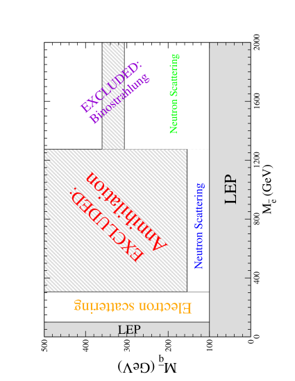
Figure 11: $M_{\tilde{e}}-M_{\tilde{q}}$ parameter space, with the regions excluded by the arguments of this paper for the case $M_{{\tilde{\chi}}}=0$ shaded. The regions already explored by LEP searches are shown in grey. The white regions indicate areas of parameter space in which we are unable to set bounds. When this is because of diffusive propagation of the neutralino we have indicated the mechanism that leads to diffusion. Values of $(M_{\tilde{e}},M_{\tilde{q}})$ in the upper-right-hand corner are permitted because there the neutralino production rate is too low to affect the SN1987A neutrino signal significantly.

The bounds shown in Fig. 11 do not change significantly with $M_{{\tilde{\chi}}}$ until masses of 50 MeV are reached. Above this value there is no squark mass bound whatsoever from SN1987A. Selectron mass bounds are also significantly reduced. For neutralinos with mass $M_{{\tilde{\chi}}}\,\,\raisebox{-3.44444pt}{$\stackrel{{\scriptstyle\textstyle>}}{{\sim}}$ }200\,{\rm MeV}$, we can essentially place no limits. Once this range of $M_{{\tilde{\chi}}}$ values is reached the LEP and Tevatron bounds on the sfermion masses, together with the Boltzmann suppression of heavy-particle production, guarantee that the supernova neutralino production rate is just too small to modify the neutrino signal markedly.

In summary, we showed that a light neutralino, $M_{{\tilde{\chi}}}<{\cal O}(1\,{\rm GeV})$ is allowed by laboratory experiments and consistent with the MSSM if it is pure bino. We have investigated the bounds obtained from the SN1987A neutrino signal on a quasi-stable neutralino with mass $M_{{\tilde{\chi}}}<200\,{\rm MeV}$ and studied the production of such neutralinos in both electron-positron annihilation and nucleon-nucleon collisions. In the former case, we compared the Raffelt criterion with an estimate of the integrated emitted energy calculated using the radial temperature and degeneracy profiles obtained in supernova simulations. We found good agreement between the two approaches. We then employed the Raffelt criterion to bound neutralino production in nucleon-nucleon collisions inside the supernova. Overall we find that for selectron masses $300\,{\rm GeV}\,\,\raisebox{-3.44444pt}{$\stackrel{{\scriptstyle\textstyle<}}{{\sim}}$ }M_{\tilde{e}}\,\,\raisebox{-3.44444pt}{$\stackrel{{\scriptstyle\textstyle<}}{{\sim}}$ }900\,{\rm GeV}$ we can exclude neutralino masses below $100\,{\rm MeV}$. On the other hand, for selectron masses above $1200\,{\rm GeV}$ there is no lower bound on the lightest neutralino mass. There is also a near absence of any bound on the squark masses: only a narrow range of $M_{\tilde{q}}$ can be excluded, and this only for $M_{{\tilde{\chi}}}\,\,\raisebox{-3.44444pt}{$\stackrel{{\scriptstyle\textstyle<}}{{\sim}}$ }20\,{\rm MeV}$.

Appendix A Appendix

In this appendix we give the explicit result for the angle-averaged hadronic tensor, $\bar{\cal H}_{ii}$, in terms of phase shifts. The quantity needed for the leading order diagrams is the nucleon–nucleon scattering T–matrix $T_{NN}$ in plane wave decomposition. It can be decomposed into partial waves in the following way. (We only give the expressions for equal final and initial spin. This is all that is required for the reaction $nn\to nn{{\tilde{\chi}}}{{\tilde{\chi}}}$.)

$$\langle S\,M_{S}^{\prime},{\bf p}\,^{\prime}|T_{NN}|S\,M_{S},{\bf p}\rangle=\sum Y_{L^{\prime}M_{L}^{\prime}}({\bf p}\,^{\prime})Y_{LM_{L}}({\bf p})^{*}{\cal T}(p,S^{\prime}\,M_{S}^{\prime},\,S\,M_{S},\,L^{\prime},\,\Delta L,M_{J})\ ,$$ (91)

where

$${\cal T}(p,S^{\prime}\,M_{S}^{\prime},\,S\,M_{S},\,L^{\prime},\,\Delta L,M_{J})=\sum\langle S^{\prime}\,M_{S}^{\prime},\,L^{\prime}\,M_{L}^{\prime}|J\,M_{J}\rangle\langle S\,M_{S},\,L\,M_{L}|J\,M_{J}\rangle\ T^{JL^{\prime}LS}(p)\ .$$ (92)

The quantity $T^{JL^{\prime}LS}(p)$ can be related to the phase shifts deduced from nucleon–nucleon scattering data directly. For example, in the case of non-coupled channels we have

$$T^{\ell}(p)=(2\pi)^{6}\left(\frac{2}{\pi Mp}\right)e^{i\delta_{\ell}(p)}\sin(\delta_{\ell}(p))\ ,$$ (93)

where $\delta_{\ell}$ denotes the phase shift in the partial wave denoted by $\ell$. These quantities are available online [45]. Note, only elastic scattering is kinematically allowed under the conditions of the study presented.

It is straight forward yet lengthy to relate $\cal T$ to the angle-averaged hadronic tensor $\bar{\cal H}_{ii}$ as defined in Eq. (71):

$$\bar{\cal H}_{ii} = \sum 2\left\{(2-M_{S}M_{S}^{\prime})|{\cal T}(p,1\,M_{S}^{\prime},\,1\,M_{S},\,L^{\prime},\,\Delta L,M_{J})|^{2}\right.$$

$$\ \qquad\left.-2\mbox{Re}\left[{\cal T}(p,1\,(M_{S}^{\prime}-1),\,1\,M_{S},\,L^{\prime},\,\Delta L,M_{J}-1)^{*}\right.\right.$$

$$\left.\left.\qquad\qquad\qquad\times{\cal T}(p,1\,M_{S}^{\prime},\,1\,(M_{S}+1),\,L^{\prime},\,\Delta L,M_{J})\right]\right\}\ .$$

References

- [1] J. Abdallah, et al., DELPHI Collaboration, DELPHI 2002-027 CONF 561. Contributed paper for ICHEP 2002, Amsterdam.
- [2] J. Polchinski, “String Theory. Vol. 1: An Introduction To The Bosonic String,” Cambridge, UK: Univ. Pr. (1998) 402 p.
- [3] D. Choudhury, H. K. Dreiner, P. Richardson and S. Sarkar, Phys. Rev. D 61 (2000) 095009 [arXiv:hep-ph/9911365].
- [4] A. Dedes, H. K. Dreiner and P. Richardson, Phys. Rev. D 65 (2002) 015001 [arXiv:hep-ph/0106199].
- [5] J. A. Grifols, E. Masso and S. Peris, Phys. Lett. B 220 (1989) 591.
- [6] J. R. Ellis, K. A. Olive, S. Sarkar and D. W. Sciama, Phys. Lett. B 215 (1988) 404.
- [7] K. Lau, Phys. Rev. D 47 (1993) 1087.
- [8] M. Kachelriess, JHEP 0002 (2000) 010 [arXiv:hep-ph/0001160].
- [9] R. Gandhi and A. Burrows, Phys. Lett. B 246 (1990) 149 [Erratum-ibid. B 261 (1991) 519].
- [10] K. Hirata et al. [KAMIOKANDE-II Collaboration], Phys. Rev. Lett. 58 (1987) 1490.
- [11] R. M. Bionta et al., Phys. Rev. Lett. 58 (1987) 1494.
- [12] G. G. Raffelt, Stars as Laboratories for Fundamental Physics, (Chicago University Press) (1996).
- [13] A. Burrows, M. S. Turner and R. P. Brinkmann, Phys. Rev. D 39, 1020 (1989).
- [14] C. Hanhart, J. A. Pons, D. R. Phillips and S. Reddy, Phys. Lett. B 509, 1 (2001) [arXiv:astro-ph/0102063].
- [15] J. R. Ellis, J. S. Hagelin, D. V. Nanopoulos, K. A. Olive and M. Srednicki, Nucl. Phys. B 238 (1984) 453.
- [16] G. Belanger, F. Boudjema, A. Pukhov and S. Rosier-Lees, arXiv:hep-ph/0212227.
- [17] D. Hooper and T. Plehn, arXiv:hep-ph/0212226.
- [18] A. Bottino, N. Fornengo and S. Scopel, arXiv:hep-ph/0212379; A. Bottino, F. Donato, N. Fornengo and S. Scopel, arXiv:hep-ph/0304080.
- [19] M. Davis, G. Efstathiou, C. S. Frenk and S. D. White, Astrophys. J. 292 (1985) 371.
- [20] H. K. Dreiner and G. G. Ross, Nucl. Phys. B 365 (1991) 597.
- [21] For a review see, for example: H. K. Dreiner, arXiv:hep-ph/9707435. For bounds on the couplings see, for example: B. C. Allanach, A. Dedes and H. K. Dreiner, Phys. Rev. D 60 (1999) 075014 [arXiv:hep-ph/9906209]; G. Bhattacharyya, Nucl. Phys. Proc. Suppl. 52A (1997) 83 [arXiv:hep-ph/9608415].
- [22] J. R. Ellis, G. B. Gelmini, J. L. Lopez, D. V. Nanopoulos and S. Sarkar, Nucl. Phys. B 373 (1992) 399.
- [23] A. Bouquet and P. Salati, Nucl. Phys. B 284 (1987) 557; H. K. Dreiner and G. G. Ross, Nucl. Phys. B 410 (1993) 188 [arXiv:hep-ph/9207221]; B. A. Campbell, S. Davidson, J. R. Ellis and K. A. Olive, Phys. Lett. B 256 (1991) 457.
- [24] B. Armbruster et al. [KARMEN Collaboration], Phys. Lett. B 348 (1995) 19.
- [25] A. Burrows and J. M. Lattimer, Astrophys. J. 307 (1986) 178.
- [26] B. L. Friman and O. V. Maxwell, Ap. J. 232, 541 (1979).
- [27] C. Hanhart, D. R. Phillips and S. Reddy, Phys. Lett. B 499, 9 (2001).
- [28] R. G. Timmermans, A. Y. Korchin, E. N. van Dalen and A. E. Dieperink, Phys. Rev. C 65, 064007 (2002).
- [29] E. N. van Dalen, A. E. Dieperink and J. A. Tjon, arXiv:nucl-th/0303037.
- [30] H. Dreiner, P. Richardson, and P. Slavich, work in preparation.
- [31] I. Gogoladze, J. Lykken, C. Macesanu and S. Nandi, arXiv:hep-ph/0211391.
- [32] Appendix E of H. E. Haber and G. L. Kane, Phys. Rept. 117 (1985) 75. Note the corrections to the differential cross section in the Erratum.
- [33] W.D. Arnett, Bull AAS, 17 (1986) 908; J.R. Wilson, in Numerical Astrophysics, ed. J. Centrella, J. LeBlanc, and R.L. Bowers (Boston: Jones & Bartlett) 1983, p.422.
- [34] Michael Kachelriess, private communication.
- [35] LEPSUSYWG, ALEPH, DELPHI, L3 and OPAL experiments, note LEPSUSYWG/02-01.1.
- [36] C. Hanhart, D. R. Phillips, S. Reddy and M. J. Savage, Nucl. Phys. B 595, 335 (2001).
- [37] S. L. Adler and Y. Dothan, Phys. Rev. 151, 1267 (1966).
- [38] F. E. Low, Phys. Rev. 110, 974 (1958).
- [39] J. F. Gunion and H. E. Haber, Nucl. Phys. B 272 (1986) 1 [Erratum-ibid. B 402 (1993) 567].
- [40] J. R. Ellis and R. A. Flores, Nucl. Phys. B 307, 883 (1988).
- [41] B. W. Filippone and X. D. Ji, arXiv:hep-ph/0101224.
- [42] W. Keil, H. T. Janka, D. N. Schramm, G. Sigl, M. S. Turner and J. R. Ellis, Phys. Rev. D 56, 2419 (1997) [arXiv:astro-ph/9612222].
- [43] G. Raffelt and D. Seckel, Phys. Rev. D 52, 1780 (1995) [arXiv:astro-ph/9312019].
- [44] R. P. Brinkmann and M. S. Turner, Phys. Rev. D 38, 2338 (1988).
- [45] R.A. Arndt, I.I. Strakovsky, and R.L. Workman, Phys. Rev. C 62, 034005(2000); CNS DAC Services, http://gwdac.phys.gwu.edu.