Study of pure annihilation type decays $B\to D_{s}^{*}K$

Abstract

In this work, we calculate the rare decays $B^{0}\to D_{s}^{*-}K^{+}$ and $B^{+}\to D_{s}^{*+}\overline{K}^{0}$ in perturbative QCD approach with Sudakov resummation. We give the branching ratio of $10^{-5}$ for $B^{0}\to D_{s}^{*-}K^{+}$, which will be tested soon in $B$ factories. The decay $B^{+}\to D_{s}^{*+}\overline{K}^{0}$ has a very small branching ratio at ${\cal O}(10^{-8})$, due to the suppression from CKM matrix elements $|V_{ub}^{*}V_{cd}|$. It may be sensitive to new physics contributions.

1 Introduction

Perturbative QCD (PQCD) method for B decays has been developed for some years [1]. It is successfully applied to exclusive $B$ meson decays recently, such as $B\to\pi\pi$ [2], $B\to K\pi$ [3], $B\to\pi\rho$ [4] and other channels [5].

Very recently, pure annihilation type B decays are discussed in the PQCD approach, such as $B^{0}\to D_{s}^{-}K^{+}$ and $B^{+}\to D_{s}^{+}\overline{K}^{0}$ [6, 7] decays and $B^{+}\to D_{s}^{+}\phi$ decay [8]. It is found that the annihilation type decay $B^{0}\to D_{s}^{-}K^{+}$ has a sizable branching ratio of $10^{-5}$, which has already been measured by experiments [6]. In this paper, we will continue to compute the branching ratios of similar decays $B^{0}\to D_{s}^{*-}K^{+}$ and $B^{+}\to D_{s}^{*+}\overline{K}^{0}$.

Because the four valence quarks in the final states $D_{s}^{*}$ and $K(\overline{K})$ are different from the ones in the $B$ meson, the rare decays $B\to D_{s}^{*}K$ are pure annihilation type decays. In the usual factorization approach (FA) [9], this decay picture is described as $B$ meson annihilating into vacuum and $D_{s}^{*}$ and $K$ meson produced from vacuum afterwards. To calculate this decay in the FA, one needs the $D_{s}^{*}\to K$ form factor at very large timelike momentum transfer ${\cal O}(M_{B})$. However the form factor at such a large momentum transfer is not known in FA. The annihilation amplitude is a phenomenological parameter in QCD factorization approach (QCDF) [10], and the QCDF calculation of these decays is also unreliable.

In this paper, we will calculate these decays in PQCD approach. Similar to the $B\to D_{S}K$ decays, the $W$ boson exchange induce the four quark operator $\bar{b}d\to\bar{c}u$ or $\bar{b}u\to\bar{d}c$, and the $\bar{s}s$ quarks included in $D_{s}^{*}K$ are produced from a gluon. This gluon attaches to any one of the quarks participating in the four quark operator. In the rest frame of $B$ meson, the produced $s$ or $\bar{s}$ quark included in $D_{s}^{*}K$ final states has $\mathcal{O}(M_{B}/4)$ momentum, and the gluon producing them has $q^{2}\sim\mathcal{O}(M_{B}^{2}/4)$. This is a hard gluon, so we can perturbatively treat the process where the four-quark operator exchanges a hard gluon with $s\bar{s}$ quark pair. It is a perturbative six quark interaction now.

In PQCD, the decay amplitude is separated into soft ($\Phi$), hard ($H$), and harder ($C$) dynamics characterized by different scales. It is conceptually written as the convolution,

$$\mbox{Amplitude}\sim\int\!\!d^{4}k_{1}d^{4}k_{2}d^{4}k_{3}\ \mathrm{Tr}\bigl{[}C(t)\Phi_{B}(k_{1})\Phi_{D_{s}^{*}}(k_{2})\Phi_{K}(k_{3})H(k_{1},k_{2},k_{3},t)\bigr{]},$$ (1)

where $k_{i}$’s are momenta of light quarks included in each meson. $C(t)$ is Wilson coefficient which results from the radiative corrections at short distance. $\Phi_{M}$ is the wave function which describes hadronization of the quark and anti-quark into the meson $M$. $H$ describes the four quark operator and the quark pair from the sea connected by a hard gluon whose scale is at the order of $M_{B}$, so the hard part $H$ can be perturbatively calculated.

Some analytic formulas for the decay amplitudes of $B\to D_{s}^{*}K$ decays will be given in the next section. In section 3, we give the numerical results and discussion. Finally, we conclude this study in section 4.

2 Analytic formulas

We consider the $B$ meson at rest for simplicity. In the light-cone coordinate, the $B$ meson momentum $P_{1}$, the $D_{s}^{*}$ meson momentum $P_{2}$ and $K$ meson momentum $P_{3}$ are taken to be:

$$P_{1}=\frac{M_{B}}{\sqrt{2}}(1,1,{\bf 0}_{T}),P_{2}=\frac{M_{B}}{\sqrt{2}}(1,r^{2},{\bf 0}_{T}),P_{3}=\frac{M_{B}}{\sqrt{2}}(0,1-r^{2},{\bf 0}_{T}),$$ (2)

where $r=M_{D_{s}^{*}}/M_{B}$ and we neglect the $K$ meson’s mass $M_{K}$. The $D_{s}^{*}$ meson’s longitudinal polarization vector $\epsilon$ is given by $\epsilon=\frac{M_{B}}{\sqrt{2}M_{D_{s}^{*}}}(1,-r^{2},{\bf 0}_{T})$. Denoting the light (anti-)quark momenta in $B$, $D_{s}^{*}$ and $K$ mesons as $k_{1}$, $k_{2}$, and $k_{3}$, respectively, we can choose $k_{1}=(x_{1}P_{1}^{+},0,{\bf k}_{1T})$, $k_{2}=(x_{2}P_{2}^{+},0,{\bf k}_{2T})$, $k_{3}=(0,x_{3}P_{3}^{-},{\bf k}_{3T})$. The decay amplitude in eq.(1) leads to:

$$\mbox{Amplitude}\sim\int\!\!dx_{1}dx_{2}dx_{3}b_{1}db_{1}b_{2}db_{2}b_{3}db_{3}\\ \mathrm{Tr}\bigl{[}C(t)\Phi_{B}(x_{1},b_{1})\Phi_{D_{s}^{*}}(x_{2},b_{2},\epsilon)\Phi_{K}(x_{3},b_{3})H(x_{i},b_{i},\epsilon,t)S_{t}(x_{i})\,e^{-S(t)}\bigr{]},$$ (3)

where $b_{i}$ is the conjugate space coordinate of $k_{iT}$, and $t$ is the largest energy scale in $H$. The large logarithms $\ln(m_{W}/t)$ coming from QCD radiative corrections to four quark operators are included in the Wilson coefficients $C(t)$. The last term, $e^{-S(t)}$, contains two kinds of logarithms. One of the large logarithms is due to the renormalization of ultra-violet divergence $\ln tb$, the other is double logarithm $\ln^{2}b$ from the overlap of collinear and soft gluon corrections. This Sudakov form factor suppresses the soft dynamics effectively [11]. Thus it makes perturbative calculation of the hard part $H$ applicable at intermediate scale, i.e.$M_{B}$ scale.

The $B$ meson wave function for incoming state and the $D_{s}^{*}$ and $K$ meson wave function for outgoing state with up to twist-3 terms are written as:

$$\Phi_{B,\alpha\beta}(x,b)=\frac{i}{\sqrt{2N_{c}}}\left[(\not\!P_{1}\gamma_{5})_{\alpha\beta}+M_{B}\gamma_{5\alpha\beta}\right]\phi_{B}(x,b),$$ (4)

$$\Phi_{D_{s}^{*},\alpha\beta}(x,b)=\frac{i}{\sqrt{2N_{c}}}\left[\not\!\epsilon(\not\!P_{2}+M_{D_{s}^{*}})_{\alpha\beta}\right]\phi_{D_{s}^{*}}(x,b),$$ (5)

$$\Phi_{K,\alpha\beta}(x_{3},b_{3}) =\frac{i}{\sqrt{2N_{c}}}\Bigl{[}\gamma_{5}\not\!P_{3}\phi_{K}^{A}(x_{3},b_{3})+m_{0K}\gamma_{5}\phi_{K}^{P}(x_{3},b_{3})$$

$$\qquad\qquad\qquad\qquad\qquad+m_{0K}\gamma_{5}(\not v\not n-1)\phi_{K}^{T}(x_{3},b_{3})\Bigr{]}_{\alpha\beta},$$ (6)

where $v=(0,1,{\bf 0}_{T})\propto P_{3}$, $n=(1,0,{\bf 0}_{T})$, and $m_{0K}=M_{K}^{2}/(m_{u}+m_{s})$.

Since the wave functions are process independent, one can use the same forms constraint by other decay channels [5] to make predictions here. Now the hard part $H$ in eq.(3) is the only channel dependent part for us to calculate perturbatively.

2.1 $B^{0}\to D_{s}^{*-}K^{+}$ decay

In the decay $B^{0}\to D_{s}^{*-}K^{+}$, the effective Hamiltonian at the scale lower than $M_{W}$ is given as [12]

$$H_{\mathrm{eff}}=\frac{G_{F}}{\sqrt{2}}V_{cb}^{*}V_{ud}\left[C_{1}(\mu)O_{1}(\mu)+C_{2}(\mu)O_{2}(\mu)\right],$$ (7)

$$O_{1}=(\bar{b}d)_{V-A}(\bar{u}c)_{V-A},\quad O_{2}=(\bar{b}c)_{V-A}(\bar{u}d)_{V-A},$$ (8)

where $C_{1,2}(\mu)$ are Wilson coefficients at renormalization scale $\mu$, and summation in $\mathrm{SU}(3)_{c}$ color’s index $\alpha$ and chiral projection, $\sum_{\alpha}\bar{q}_{\alpha}\gamma^{\nu}(1-\gamma_{5})q^{\prime}_{\alpha}$ are abbreviated to $(\bar{q}q^{\prime})_{V-A}$. The lowest order diagrams of $B^{0}\to D_{s}^{*-}K^{+}$ are drawn in Fig.1 according to this effective Hamiltonian. There are altogether four quark diagrams. Just as what we said above, the decay $B\to D_{s}^{*}K$ only has annihilation diagrams.

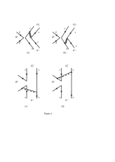
Figure 1: Diagrams for $B^{0}\to D_{s}^{*-}K^{+}$ decay. The factorizable diagrams (a),(b) contribute to $F_{a}^{(2)}$, and nonfactorizable (c), (d) do to $M_{a}$.

By calculating the hard part $H$ at the first order of $\alpha_{s}$, we get the following analytic formulas. With the meson wave functions, the amplitude for the factorizable annihilation diagrams in Fig.1(a) and (b) results in $F_{a}^{(i=2)}$ as:

$$F_{a}^{(i)}=-16\pi C_{F}M_{B}^{2}\int_{0}^{1}\!\!dx_{2}dx_{3}\int_{0}^{\infty}\!\!b_{2}db_{2}\,b_{3}db_{3}\ \phi_{D_{s}^{*}}(x_{2},b_{2})\\ \times\Bigl{[}\bigl{\{}(1-r^{2})\left(1-(1-r^{2})x_{3}\right)\phi_{K}^{A}(x_{3},b_{3})+r(1-r^{2})x_{3}r_{K}\phi_{K}^{P}(x_{3},b_{3})\\ -r(1+r^{2})r_{K}\phi_{K}^{T}(x_{3},b_{3})\bigr{\}}E_{f}^{i}(t_{a}^{1})h_{a}(x_{2},x_{3},b_{2},b_{3})-\bigl{\{}(1-r^{2})x_{2}\phi_{K}^{A}(x_{3},b_{3})\\ +2r(1-r^{2}-x_{2})r_{K}\phi_{K}^{P}(x_{3},b_{3})\bigr{\}}E_{f}^{i}(t_{a}^{2})h_{a}(1-x_{3},1-x_{2},b_{3},b_{2})\Bigr{]}.$$ (9)

In the function, $C_{F}=4/3$ is the group factor of $\mathrm{SU}(3)_{c}$, and $r_{K}=m_{0K}/M_{B}$. The functions $E_{f}^{i}$, $t_{a}^{1,2}$, $h_{a}$ will be given in the appendix. The distribution amplitudes $\phi_{M}$, are given in the next section. The amplitude for the nonfactorizable annihilation diagrams in Fig.1(c) and (d) results in

$$M_{a}=\frac{1}{\sqrt{2N_{c}}}64\pi C_{F}M_{B}^{2}\int_{0}^{1}\!\!dx_{1}dx_{2}dx_{3}\int_{0}^{\infty}\!\!b_{1}db_{1}\,b_{2}db_{2}\ \phi_{B}(x_{1},b_{1})\phi_{D_{s}^{*}}(x_{2},b_{2})\\ \times\Bigl{[}\bigl{\{}(1-r^{2})\left((1-r^{2})(1-x_{3})-r^{2}x_{2}\right)\phi_{K}^{A}(x_{3},b_{2})\\ -r\left(x_{2}-(1-r^{2})(1-x_{3})\right)r_{K}\phi_{K}^{P}(x_{3},b_{2})\\ -r\left(x_{2}+(1-r^{2})(1-x_{3})\right)r_{K}\phi_{K}^{T}(x_{3},b_{2})\bigr{\}}E_{m}(t_{m}^{1})h_{a}^{(1)}(x_{1},x_{2},x_{3},b_{1},b_{2})\\ -\bigl{\{}(1-r^{2})\left((1-r^{2})x_{2}+r^{2}\right)\phi_{K}^{A}(x_{3},b_{2})\\ +r(x_{2}-(1-r^{2})(1-x_{3}))r_{K}\phi_{K}^{P}(x_{3},b_{2})\\ +r(x_{2}-2r^{2}-(1-r^{2})(1+x_{3}))r_{K}\phi_{K}^{T}(x_{3},b_{2})\bigr{\}}E_{m}(t_{m}^{2})h_{a}^{(2)}(x_{1},x_{2},x_{3},b_{1},b_{2})\Bigr{]},$$ (10)

where $x_{1}$ dependence in the numerators of the hard part are neglected by the assumption $x_{1}\ll x_{2},x_{3}$.

Comparing with $B^{0}\to D_{s}^{-}K^{+}$ [6], we find that the leading twist contribution, which is proportional to $\phi_{K}^{A}$, is almost the same. However the subleading twist contribution, which is proportional to $r~{}r_{K}$, change significantly, especially for the $\phi_{K}^{P}(x_{3},b_{2})$ terms in (9) and (10).

The total decay amplitude for $B^{0}\to D_{s}^{*-}K^{+}$ decay is given as $A=f_{B}F_{a}^{(2)}+M_{a}$. The decay width is then

$$\Gamma(B^{0}\to D_{s}^{*-}K^{+})=\frac{G_{F}^{2}M_{B}^{3}}{128\pi}(1-r^{2})|V_{cb}^{*}V_{ud}A|^{2}.$$ (11)

The charge conjugate decay $\overline{B}^{0}\to D_{s}^{*+}K^{-}$ is the same value as $B^{0}\to D_{s}^{*-}K^{+}$ just because $|V_{cb}^{*}V_{ud}|$ is the same as $|V_{cb}V_{ud}^{*}|$. Since there is only one kind of CKM phase involved in the decay, there is no CP violation in the standard model for this decay channel.

2.2 $B^{+}\to D_{s}^{*+}\overline{K}^{0}$ decay

The effective Hamiltonian related to $B^{+}\to D_{s}^{*+}\overline{K}^{0}$ decay is given as [12]

$$H_{\mathrm{eff}}=\frac{G_{F}}{\sqrt{2}}V_{ub}^{*}V_{cd}\left[C_{1}(\mu)O_{1}(\mu)+C_{2}(\mu)O_{2}(\mu)\right],$$ (12)

$$O_{1}=(\bar{b}d)_{V-A}(\bar{c}u)_{V-A},\quad O_{2}=(\bar{b}u)_{V-A}(\bar{c}d)_{V-A}.$$ (13)

The amplitude for the factorizable annihilation diagrams results in $-F_{a}^{(i=1)}$. The amplitude for the nonfactorizable annihilation diagrams is given as

$$M_{a}^{\prime}=\frac{1}{\sqrt{2N_{c}}}64\pi C_{F}M_{B}^{2}\int_{0}^{1}\!\!\!dx_{1}dx_{2}dx_{3}\int_{0}^{\infty}\!\!\!\!\!b_{1}db_{1}\,b_{2}db_{2}\ \phi_{B}(x_{1},b_{1})\phi_{D_{s}^{*}}(x_{2},b_{2})\\ \times\Bigl{[}\bigl{\{}(1-2r^{2})x_{2}\phi_{K}^{A}(x_{3},b_{2})+r\left(x_{2}-(1-r^{2})(1-x_{3})\right)r_{K}\phi_{K}^{P}(x_{3},b_{2})\\ +r\left(x_{2}+(1-r^{2})(1-x_{3})\right)r_{K}\phi_{K}^{T}(x_{3},b_{2})\bigr{\}}E_{m}^{\prime}(t_{m}^{1})h_{a}^{(1)}(x_{1},x_{2},x_{3},b_{1},b_{2})\\ -\bigl{\{}(1-r^{2})\left(1-x_{2}r^{2}-(1-r^{2})x_{3}\right)\phi_{K}^{A}(x_{3},b_{2})\\ -r\left(x_{2}-(1-r^{2})(1-x_{3})\right)r_{K}\phi_{K}^{P}(x_{3},b_{2})\\ -r\left(x_{2}-2r^{2}-(1-r^{2})(1-x_{3})\right)r_{K}\phi_{K}^{T}(x_{3},b_{2})\bigr{\}}E_{m}^{\prime}(t_{m}^{2})h_{a}^{(2)}(x_{1},x_{2},x_{3},b_{1},b_{2})\Bigr{]}.$$ (14)

Comparing with the decay to two pseudo-scaler final states $B^{+}\to D_{s}^{+}\overline{K}^{0}$ [6], the change only occur in $r^{2}$ terms. Therefore, the non-factorizable contribution in $B^{+}$ decay does not change much.

The total decay amplitude $A^{\prime}$ and decay width $\Gamma$ for $B^{+}\to D_{s}^{*+}\overline{K}^{0}$ decay are given as

$$A^{\prime}=-f_{B}F_{a}^{(1)}+M_{a}^{\prime},$$ (15)

$$\Gamma(B^{+}\to D_{s}^{*+}\overline{K}^{0})=\frac{G_{F}^{2}M_{B}^{3}}{128\pi}(1-r^{2})|V_{ub}^{*}V_{cd}A^{\prime}|^{2}.$$ (16)

The decay width for CP conjugated mode, $B^{-}\to D_{s}^{*-}K^{0}$, is the same value as $B^{+}\to D_{s}^{*+}\overline{K}^{0}$. Similar to the $B^{0}$ decay, there is also no CP violation in this decay within standard model.

3 Numerical evaluation

We use the wave function of $B$ meson written as [5]

$$\phi_{B}(x,b)=N_{B}x^{2}(1-x)^{2}\exp\left[-\frac{M_{B}^{2}\ x^{2}}{2\omega_{b}^{2}}-\frac{1}{2}(\omega_{b}b)^{2}\right],$$ (17)

where $N_{B}$ is a normalization factor. Because the mass difference between $D_{s}$ and $D_{s}^{*}$ is not large, for simplicity, their wave functions are chosen to be the same [5, 6]:

$$\phi_{D_{s}^{*}}(x,b)=\frac{3}{\sqrt{2N_{c}}}f_{D_{s}^{*}}x(1-x)\{1+a_{D_{s}^{*}}(1-2x)\}\exp\left[-\frac{1}{2}(\omega_{D_{s}^{*}}b)^{2}\right].$$ (18)

Since $c$ quark is much heavier than $s$ quark, this function is peaked at $c$ quark side, i.e. small $x$ region.

The $K$ meson wave functions are given as

$$\phi_{K}^{A}(x) = \frac{f_{K}}{2\sqrt{2N_{c}}}6x(1-x)\left\{1-a_{1}^{K}\cdot 3\xi+a_{2}^{K}\cdot\frac{3}{2}(-1+5\xi^{2})\right\},$$ (19)

$$\phi_{K}^{P}(x) = \frac{f_{K}}{2\sqrt{2N_{c}}}\left\{1+a_{p1}^{K}\cdot\frac{1}{2}(-1+3\xi^{2})+a_{p2}^{K}\cdot\frac{1}{8}(3-30\xi^{2}+35\xi^{4})\right\},$$ (20)

$$\phi_{K}^{T}(x) = \frac{f_{K}}{2\sqrt{2N_{c}}}(1-2x)\left\{1+a_{T}^{K}\cdot 3(-3+5\xi^{2})\right\},$$ (21)

where $\xi=2x-1$. The parameters of these distribution amplitudes calculated from QCD sum rule [13] are given as

$$a_{1}^{K}=0.17,\quad a_{2}^{K}=0.2,\quad a_{p1}^{K}=0.212,\quad a_{p2}^{K}=-0.148,\quad a_{T}^{K}=0.0527,$$ (22)

for $m_{0K}=1.6\mbox{ GeV}$. In addition, we use the following input parameters [6]:

$$f_{B}=190\mbox{ MeV},\ f_{K}=160\mbox{ MeV},\ f_{D_{s}^{*}}=241\mbox{ MeV},$$ (23)

$$m_{0K}=1.6\mbox{ GeV},\ \omega_{b}=0.4\mbox{ GeV},\ a_{D_{s}^{*}}=0.3,\ \omega_{D_{s}^{*}}=0.3\mbox{ GeV}.$$ (24)

For branching ratio estimation, we use the CKM matrix elements and the lifetimes of B mesons as following [14],

$$|V_{ud}|=0.9734,\ |V_{ub}|=3.6\times 10^{-3},$$ (25)

$$|V_{cb}|=41.2\times 10^{-3},\ |V_{cd}|=0.224,$$ (26)

$$\tau_{B^{\pm}}=1.67\times 10^{-12}\mbox{ s,}\quad\tau_{B^{0}}=1.54\times 10^{-12}\mbox{ s}.$$ (27)

The predicted branching ratios are

$$\mathrm{Br}(B^{0}\to D_{s}^{*-}K^{+})=2.7\times 10^{-5},$$ (28)

$$\mathrm{Br}(B^{+}\to D_{s}^{*+}\overline{K}^{0})=4.0\times 10^{-8}.$$ (29)

The branching ratio of $B^{+}\to D_{s}^{*+}\overline{K}^{0}$ is much smaller than that of $B^{0}\to D_{s}^{*-}K^{+}$, due to the suppression from CKM matrix element $\mid V_{ub}^{*}V_{cd}\mid<<|V_{cb}^{*}V_{ud}|$. C-H Chen has also given the branching ratio of $B^{0}\to D_{s}^{*-}K^{+}$ [7], our result agrees with his.

In these processes of $B\to D_{s}^{*}K$, only the longitudinal polarization of $D_{s}^{*}$ has contribution. If we ignore the difference between $f_{D_{s}}$ and $f_{D_{s}^{*}}$ and the difference between $M_{D_{s}}$ and $M_{D_{s}^{*}}$, the branch ratios are thought to be the same as the corresponding $B\to D_{s}K$ decays. But in fact the branching ratio of $B^{0}\to D_{s}^{*-}K^{+}$ is a little smaller than that of $B^{0}\to D_{s}^{-}K^{+}$, because the contribution of twist-3 wave function in $B^{0}\to D_{s}^{*-}K^{+}$ decay become negative. Although the larger $f_{D_{s}^{*}}$ makes the branching ratio larger, a larger $M_{D_{s}^{*}}$ leads to a smaller branching ratio. The effect of $M_{D_{s}^{*}}$ is more dominant than that of $f_{D_{s}^{*}}$. In decays of charged $B^{+}$, $f_{D_{s}^{*}}$ makes branching ratios larger, and $M_{D_{s}^{*}}$ has little effect, such that the $B^{+}\to D_{s}^{*+}\bar{K}^{0}$ decay in this case has a little larger branching ratio than $B^{+}\to D_{s}^{+}\bar{K}^{0}$.

For the experimental side, there are only upper limits given at $90$% confidence level [14],

$$\mathrm{Br}(B^{0}\to D_{s}^{*-}K^{+}) <1.7\times 10^{-4},$$ (30)

$$\mathrm{Br}(B^{+}\to D_{s}^{*+}\overline{K}^{0}) <1.1\times 10^{-3}.$$ (31)

Obviously, our results are consistent with the data.

In addition to the perturbative annihilation contributions, there is also a hadronic picture for the $B^{0}\to D_{s}^{*-}K^{+}$. The $B$ meson decays into $D^{-}$ and $\rho^{+}$, the secondary particles then exchanging a $K^{0}$, scatter into $D_{s}^{*-}$, $K^{+}$ through final state interaction afterwards. For charged decay, $B^{+}$ meson decays into $D^{0}\rho^{+}$ then scatter into $D_{s}^{*+}$ and $\bar{K}^{0}$ by exchanging a $K^{+}$. But this picture can not be calculated accurately. In [6], the results from PQCD approach for $B^{0}\to D_{s}^{-}K^{+}$ decay were consistent with the experiment, which shows that the soft final state interaction may not be important.

The calculated branching ratios in PQCD are sensitive to various parameters, such as parameters in eqs.(22-24). It is necessary to give the sensitivity of the branching ratios when we choose the parameters to some extent. Table 1 shows the sensitivity of the branch ratios to $30$% change of $a_{D_{s}^{*}}$, $\omega_{D_{s}^{*}}$ and $\omega_{b}$. Here we don’t present the sensitivity to $a_{p1,p2,T}^{K}$ because the branching ratios are insensitive to them. It is found that the uncertainty of the predictions on PQCD is mainly due to $\omega_{D_{s}^{*}}$, which characterizes the shape of $D_{s}^{*}$ wave function.

Table 1: The sensitivity of the decay branching ratios to $30$% change of $\omega_{D_{s}^{*}}$, $a_{D_{s}^{*}}$ and $\omega_{b}$.

	$(10^{-5})$	$(10^{-8})$
$\omega_{D_{s}^{*}}$	$\mathrm{Br}(B^{0}\to D_{s}^{*-}K^{+})$	$\mathrm{Br}(B^{+}\to D_{s}^{*+}\overline{K}^{0})$
$0.21$	$3.17$	$4.66$
$0.30$	$2.65$	$3.95$
$0.39$	$2.11$	$3.20$
$a_{D_{s}^{*}}$	$\mathrm{Br}(B^{0}\to D_{s}^{*-}K^{+})$	$\mathrm{Br}(B^{+}\to D_{s}^{*+}\overline{K}^{0})$
$0.21$	$2.40$	$3.68$
$0.30$	$2.65$	$3.95$
$0.39$	$2.92$	$4.24$
$\omega_{b}$	$\mathrm{Br}(B^{0}\to D_{s}^{*-}K^{+})$	$\mathrm{Br}(B^{+}\to D_{s}^{*+}\overline{K}^{0})$
$0.21$	$3.12$	$3.87$
$0.40$	$2.65$	$3.95$
$0.52$	$2.31$	$4.18$

From the above discussions, we can derive the uncertainties of the branching ratios within the suitable ranges on $\omega_{D_{s}^{*}}$, $a_{D_{s}^{*}}$ and $\omega_{b}$. The branching ratios normalized by the decay constants and the CKM matrix elements result in

$$\mathrm{Br}(B^{0}\to D_{s}^{*-}K^{+})=(2.7\pm 0.6)\times 10^{-5}\left(\frac{f_{B}\ f_{D_{s}^{*}}}{190\mbox{ MeV}\cdot 240\mbox{ MeV}}\right)^{2}\left(\frac{|V_{cb}^{*}\ V_{ud}|}{0.0412\cdot 0.9734}\right)^{2},$$ (32)

$$\mathrm{Br}(B^{+}\to D_{s}^{*+}\overline{K}^{0})=(4.0\pm 0.8)\times 10^{-8}\left(\frac{f_{B}\ f_{D_{s}^{*}}}{190\mbox{ MeV}\cdot 240\mbox{ MeV}}\right)^{2}\left(\frac{|V_{ub}^{*}\ V_{cd}|}{0.0036\cdot 0.224}\right)^{2}.$$ (33)

4 Conclusion

In this paper, we calculate the $B^{0}\to D_{s}^{*-}K^{+}$ and $B^{+}\to D_{s}^{*+}\overline{K}^{0}$ decays in PQCD approach. These two decays occur purely via annihilation type diagrams because the four quarks in final states are not the same as the ones in $B$ meson. We argue that the soft final state interaction may be small in B decays. The PQCD calculation of annihilation decays is reliable. The branching ratio for $B^{0}\to D_{s}^{*-}K^{+}$ decay is sizable at order of $10^{-5}$, which can be measured in the current $B$ factories Belle and BABAR. The small branching ratio of $B^{+}\to D_{s}^{*+}\bar{K}^{0}$ ($10^{-8}$) predicted in the SM, makes it sensitive to new physics contributions, which may be studied in the future LHC-B experiment.

Appendix A Some formulas used in the text

The function $E_{f}^{i}$, $E_{m}$, and $E^{\prime}_{m}$ including Wilson coefficients are defined as

$$E_{f}^{i}(t)=a_{i}(t)\alpha_{s}(t)\,e^{-S_{D}(t)-S_{K}(t)},$$ (34)

$$E_{m}(t)=C_{2}(t)\alpha_{s}(t)\,e^{-S_{B}(t)-S_{D}(t)-S_{K}(t)},$$ (35)

$$E_{m}^{\prime}(t)=C_{1}(t)\alpha_{s}(t)\,e^{-S_{B}(t)-S_{D}(t)-S_{K}(t)},$$ (36)

where

$$a_{1}(t)={C_{1}(t)}/{3}+C_{2}(t),\quad a_{2}(t)=C_{1}(t)+{C_{2}(t)}/3,$$ (37)

and $S_{B}$, $S_{D}$, and $S_{K}$ result from summing both double logarithms caused by soft gluon corrections and single ones due to the renormalization of ultra-violet divergence. Those factors are given in ref. [5, 6]. In the numerical analysis we use leading logarithms expressions for Wilson coefficients $C_{1,2}$ presented in ref.[12, 2].

The functions $h_{a}$, $h_{a}^{(1)}$, and $h_{a}^{(2)}$ in the decay amplitudes consist of two parts: one is the jet function $S_{t}(x_{i})$ derived by the threshold resummation [15], the other is the propagator of virtual quark and gluon. They are defined by

$$h_{a}(x_{2},x_{3},b_{2},b_{3})=S_{t}(1-x_{3})\left(\frac{\pi i}{2}\right)^{2}H_{0}^{(1)}(M_{B}\sqrt{(1-r^{2})x_{2}(1-x_{3})}\,b_{2})$$

$$\times\left\{H_{0}^{(1)}(M_{B}\sqrt{(1-r^{2})(1-x_{3})}\,b_{2})J_{0}(M_{B}\sqrt{(1-r^{2})(1-x_{3})}\,b_{3})\theta(b_{2}-b_{3})+(b_{2}\leftrightarrow b_{3})\right\},$$ (38)

$$h^{(j)}_{a}(x_{1},x_{2},x_{3},b_{1},b_{2})=$$

$$\biggl{\{}\frac{\pi i}{2}\mathrm{H}_{0}^{(1)}(M_{B}\sqrt{(1-r^{2})x_{2}(1-x_{3})}\,b_{1})\mathrm{J}_{0}(M_{B}\sqrt{(1-r^{2})x_{2}(1-x_{3})}\,b_{2})\theta(b_{1}-b_{2})$$

$$\qquad\qquad\qquad\qquad+(b_{1}\leftrightarrow b_{2})\biggr{\}}\times\left(\begin{matrix}\mathrm{K}_{0}(M_{B}F_{(j)}b_{1}),&\text{for}\quad F^{2}_{(j)}>0\\ \frac{\pi i}{2}\mathrm{H}_{0}^{(1)}(M_{B}\sqrt{|F^{2}_{(j)}|}\ b_{1}),&\text{for}\quad F^{2}_{(j)}<0\end{matrix}\right),$$ (39)

where $\mathrm{H}_{0}^{(1)}(z)=\mathrm{J}_{0}(z)+i\,\mathrm{Y}_{0}(z)$, and $F_{(j)}$s are defined by

$$F^{2}_{(1)}=(1-r^{2})(x_{1}-x_{2})(1-x_{3}),\ F^{2}_{(2)}=x_{1}+x_{2}+(1-r^{2})(1-x_{1}-x_{2})(1-x_{3}).$$ (40)

We adopt the parametrization for $S_{t}(x)$ of the factorizable contributions,

$$S_{t}(x)=\frac{2^{1+2c}\Gamma(3/2+c)}{\sqrt{\pi}\Gamma(1+c)}[x(1-x)]^{c},\quad c=0.3,$$ (41)

which is proposed in ref. [16]. The hard scale $t$’s in the amplitudes are taken as the largest energy scale in the hard part $H$ to kill the large logarithmic radiative corrections:

$$t_{a}^{1}=\mathrm{max}(M_{B}\sqrt{(1-r^{2})(1-x_{3})},1/b_{2},1/b_{3}),$$ (42)

$$t_{a}^{2}=\mathrm{max}(M_{B}\sqrt{(1-r^{2})x_{2}},1/b_{2},1/b_{3}),$$ (43)

$$t_{m}^{j}=\mathrm{max}(M_{B}\sqrt{|F^{2}_{(j)}|},M_{B}\sqrt{(1-r^{2})x_{2}(1-x_{3})},1/b_{1},1/b_{2}).$$ (44)

References

- [1] G.P. Lepage and S. Brosky, Phys. Rev. D22, 2157 (1980); J. Botts and G. Sterman, Nucl. Phys. B225, 62 (1989).
- [2] C.-D. Lü, K. Ukai and M.-Z. Yang, Phys. Rev. D63, 074009 (2001).
- [3] Y.-Y. Keum, H.-n. Li and A. I. Sanda, Phys. Lett. B504, 6 (2001); Phys. Rev. D63, 054008 (2001).
- [4] C.-D. Lü and M.Z. Yang, Eur. Phys. J. C23, 275 (2002).
- [5] H.-n. Li, Phys. Rev. D64, 014019 (2001); S. Mishima, Phys. Lett. B521, 252 (2001); E. Kou and A.I. Sanda, Phys. Lett. B525, 240 (2002); C.-H. Chen, Y.-Y. Keum, and H.-n. Li, Phys. Rev. D64, 112002 (2001); A.I. Sanda and K. Ukai, Prog. Theor. Phys. 107, 421 (2002); C.-H. Chen, Y.-Y. Keum, and H.-n. Li, Phys. Rev. D66, 054013 (2002); M. Nagashima and H.-n. Li, hep-ph/0202127; Y.-Y. Keum, hep-ph/0209002; hep-ph/0209208(to appear in PRL); hep-ph/0210127; Y.-Y. Keum and A. I. Sanda, Phys. Rev. D67, 054009 (2003); C.D. Lü, M.Z. Yang, hep-ph/0212373, to appear in Eur. Phys. J. C.
- [6] K. Ukai, 287-290, Preceedings for 4th International Conference on B Physics and CP Violation (BCP4), Japan, 2001; C.-D. Lü and K. Ukai, hep-ph/0210206, to appear in Eur. Phys. J. C.
- [7] C.-H. Chen, hep-ph/0301154.
- [8] C.D. Lü, Eur. Phys. J. C24, 121 (2002).
- [9] M. Wirbel, B. Stech, M. Bauer, Z. Phys. C29, 637 (1985); M. Bauer, B. Stech, M. Wirbel, Z. Phys. C34, 103 (1987); A. Ali, G. Kramer and C.D. Lü, Phys. Rev. D58, 094009 (1998); C.D. Lü, Nucl. Phys. Proc. Suppl. 74, 227-230 (1999); Y.-H. Chen, H.-Y. Cheng, B. Tseng, K.-C. Yang, Phys. Rev. D60, 094014 (1999).
- [10] M. Beneke, G. Buchalla, M. Neubert, C.T. Sachrajda, Phys. Rev. Lett. 83, 1914 (1999); Nucl. Phys. B591, 313 (2000).
- [11] H.-n. Li and B. Tseng, Phys. Rev. D57, 443, (1998).
- [12] G. Buchalla, A. J. Buras and M. E. Lautenbacher, Rev. Mod. Phys. 68, 1125 (1996).
- [13] P. Ball, JHEP, 09, 005, (1998); JHEP, 01, 010, (1999).
- [14] Review of Particle Physics, K. Hagiwara et al., Phys. Rev. D66, 010001 (2002).
- [15] H.-n. Li, hep-ph/0102013 (to appear in PRD).
- [16] T. Kurimoto, H.-n. Li, and A. I. Sanda, Phys. Rev. D65, 014007 (2002).