Chern-Simons production during preheating in hybrid inflation models
Abstract
We study the onset of symmetry breaking after hybrid inflation in a model having the field content of the SU(2) gauge-scalar sector of the standard model, coupled to a singlet inflaton. This process is studied in (3+1)-dimensions in a fully nonperturbative way with the help of lattice techniques within the classical approximation. We focus on the role played by gauge fields and, in particular, on the generation of Chern-Simons number. Our results are shown to be insensitive to the various cutoffs introduced in our numerical approach. The spectra preserves a large hierarchy between long and short-wavelength modes during the whole period of symmetry breaking and Chern-Simons generation, confirming that the dynamics is driven by the low momentum sector of the theory. We establish that the Chern-Simons production mechanism is associated with local sphaleron-like structures. The corresponding sphaleron rates are of order , which, within certain scenarios of electroweak baryogenesis and a (not unnaturally large) additional source of CP violation, could explain the present baryon asymmetry of the Universe.
pacs:
98.80.CqPreprint FT-UAM-03/07, IFT-UAM/CSIC-03-13, hep-ph/0304285
I Introduction
Everything we see in the Universe, from planets and stars, to galaxies and clusters of galaxies, is made out of matter, so where did the antimatter in the Universe go? Is this the result of an accident, a contingency during the evolution of the Universe, or is it an inevitable consequence of some asymmetry in the laws of nature? Theorists tend to believe that the observed excess of matter over antimatter, , comes from tiny differences in their fundamental interactions soon after the end of inflation.
It has been known since Sakharov’s work that there are three necessary (but not sufficient) conditions for the baryon asymmetry of the Universe to develop sakharov . First, we need interactions that do not conserve baryon number B, otherwise no asymmetry could be produced in the first place. Second, C and CP symmetry must be violated, in order to differentiate between matter and antimatter, otherwise B nonconserving interactions would produce baryons and antibaryons at the same rate, thus maintaining zero net baryon number. Third, these processes should occur out of thermal equilibrium, otherwise the net baryon number cannot change in time.
The possibility that baryogenesis could have occurred at the electroweak scale is very appealing RS . The Standard Model is baryon symmetric at the classical level, but violates B at the quantum level, through the chiral anomaly. Electroweak (EW) interactions violate C and CP through the irreducible phase in the Cabibbo-Kobayashi-Maskawa (CKM) matrix, but the magnitude of the violation is probably insufficient to account for the observed baryon asymmetry RS .
One of the most appealing mechanisms for generating the baryon asymmetry of the Universe makes use of the nonperturbative baryon-number-violating sphaleron interactions present in the electroweak model at high temperatures KRS . The usual scenario invokes a strongly first-order phase transition to drive the primordial plasma out of equilibrium and set the stage for baryogenesis. This scenario presupposes that the Universe was in thermal equilibrium before and after the electroweak phase transition, and far from it during the phase transition. Although there is a mounting evidence in support of the standard Big-Bang theory up to nucleosynthesis temperatures of MeV), the assumption that the Universe was in thermal equilibrium at earlier times is merely a result of a (plausible) theoretical extrapolation. Furthermore, the electroweak phase transition is certainly not first order Rummukainen , given the present lower bound on the mass of the Higgs boson PDG . In order to account for the observed baryon asymmetry and to prevent the later baryon wash-out, a stronger deviation from thermal equilibrium is required leptogenesis .
According to recent studies of reheating after inflation, the Universe could have undergone a period of “preheating” KLS , during which only certain modes are highly populated, and the Universe remains for some time very far from thermal equilibrium nonthermal . Recently, a new mechanism for electroweak baryogenesis was proposed GGKS ; KT , based on the nonperturbative production of long-wavelength gauge and Higgs field configurations via parametric resonance at the end of inflation. Such mechanism occurs very far from equilibrium and could be very efficient in producing the baryon asymmetry of the Universe at the EW scale. The very nonequilibrium nature of preheating may facilitate the baryon number generation, due to the sustained coherent oscillations of the scalar fields involved GBG ; JGB ; Dima ; CGK .
The proposed scenario suggests a picture of the early Universe in which thermal equilibrium is maintained only up to temperatures of GeV). The earlier history of the Universe is diluted by a low-scale period of inflation, after which the Universe never reheated above the electroweak scale. It is not easy to construct a natural model of low-scale inflation. The main problem is to achieve the extreme flatness of the effective potential in the inflaton direction (i.e. the smallness of the inflaton mass in the false vacuum) without fine-tuning Lyth . Although several models have been proposed, the lack of naturalness remains a serious problem. Perhaps recent ideas related to large internal dimensions can provide a solution Creminelli . We will not be concerned with such issues here. The only qualitative feature of the low-energy inflation model that is essential to us is that it provides a “cold” state as initial condition for EW symmetry breaking. The main question to be addressed here is whether electroweak baryogenesis can take place under these circumstances.
As a specific model, a gauged Higgs-inflaton model of hybrid inflation was considered in Ref. GGKS . In this model the inflaton is a singlet coupled only to the Higgs boson, and induces dynamical electroweak symmetry breaking as it slow-rolls below a critical value. The false vacuum energy is quickly converted into a Higgs condensate with large occupation numbers, in a process known as “tachyonic preheating” GBKLT . The system evolves toward equilibrium while slowly populating higher and higher momentum modes TK . The expansion of the Universe at the electroweak scale is negligible compared to the mass scales involved, so the energy density is conserved, and the final reheating temperature is solely determined by the energy stored initially in the inflaton field, that is, the false vacuum energy density.
To make a quantitative test of the proposal, a (1+1)-dimensional Abelian Higgs model GRS ; 1p1 was studied in Ref. GGKS . It contains all the relevant ingredients: an anomalous current which relates the (1+1)-topological U(1) winding number to the global charge (baryon number), plus a CP-violating operator dependent upon the Higgs expectation value. In Ref. GGKS the scenario was shown to be very efficient in preventing the baryon wash-out, thanks to the coherent oscillations of the Higgs condensate GBG . Although the results are very encouraging, they do not yet prove the validity of the scenario since there might be specific signatures in (3+1)-dimensions which prevent the production of baryons. Other authors have also studied this (1+1) dimensional model ST ; ST2 ; CPR , with similar conclusions regarding the generation of baryon number asymmetry, but with different points of view concerning its origin.
Since then, there have been several papers studying this scenario in (3+1)-dimensions. It was shown in Ref. GBKLT that preheating does not proceed after hybrid inflation via parametric resonance, but through spinodal instability, which induces the tachyonic growth of the long-wavelength Higgs modes. The first studies were done in the quench approximation GBKLT ; GBRM , and later in the complete hybrid inflation scenario with a time-dependent Higgs mass JGB ; ABC ; CPR ; GGG . These studies suggest that preheating in hybrid inflation models can be very efficient in producing Higgs semiclassical modes at the electroweak symmetry breaking. Most of these papers consider only the purely scalar sector. However, in Ref. CPR an Abelian gauge field was introduced to study the topological defect formation. Non-Abelian gauge fields with different initial conditions were considered in Ref. RSC and in a set-up similar to ours in Refs. ST2 ; SST .
The detailed way in which symmetry breaking occurs at the end of hybrid inflation was analyzed with a (3+1)-lattice simulation in Ref. GGG , from now on referred to as paper I. In that paper, we considered the hybrid model in the absence of gauge fields. We studied the early stages of the dynamics of the Higgs modes, evolving from quantum to classical behavior, and the subsequent nonperturbative evolution through symmetry breaking. This process is mediated by the formation and growth of lumps, which later develop into bubbles (or spherical shock waves) and their subsequent collision leads the way toward thermalization. However, it is expected that the gauge fields play an important role in the process of electroweak symmetry breaking. Furthermore, the relevance of gauge fields in our context is connected to the generation of Chern-Simons (CS) number, which, via the chiral anomaly, may induce baryon production in the presence of a CP-violating interaction.
In the present paper we address a detailed study of the post-inflation dynamics of the hybrid model in (3+1) dimensions, including non-Abelian gauge fields. We will study the evolution of this model from the initial conditions suggested by hybrid inflation, through the tachyonic preheating stage on the way toward full thermalization. Our main goal will be to analyze the generation of Chern-Simons number in this process. It is expected that after inclusion of a CP-violating operator, this will generate the required baryon asymmetry. However, in this paper we are not including such a term, which we postpone for future work. Another possible improvement to our model is the inclusion of the full SU(2)U(1) gauge group. However, as generally assumed, the simplified SU(2) model suffices to describe the sphaleron transitions and Chern-Simons number production RS .
From the methodological point of view, our paper clarifies the importance of setting the right initial conditions of the non-Abelian gauge fields for the study of baryogenesis at preheating after inflation. In a recent paper moore , Guy Moore challenged the viability of lattice methods for testing the scenario of Ref. GGKS . He argued that the classical evolution of the gauge fields produced spectra that were soon dominated by high-momentum modes and thus prone to large lattice systematic errors. As we will show, this is not the case when the appropriate set of initial conditions for both the Higgs and gauge fields is chosen. The spectra of all fields involved remain strongly hierarchical, with the occupation of long-wave modes several orders of magnitude larger than that of the dangerous high-momentum modes throughout its evolution at symmetry breaking and beyond the region of interest for Chern-Simons number production. Moreover, our results are stable under changes of the cutoffs introduced in the procedure, thus providing a consistent framework for analyzing the real-time evolution of the inflaton-Higgs-gauge model.
The paper is organized as follows. In Section II we describe the hybrid model which we will study. We also give a brief explanation of our choice of parameters, and of our post-inflation initial conditions. In Section III we describe the methodology used to study the dynamics of this system through symmetry breaking. First, we give a short recollection of our results in paper I, which show the fast growth of certain Higgs modes and their transition from quantum to classical behavior. This stage sets the stochastic initial conditions for the subsequent classical real time evolution of the full inflaton-Higgs-gauge system. Then, we describe our use of lattice techniques to approach the latter problem, as well as the specific modifications necessary to handle the initial conditions in the presence of gauge fields. To facilitate reading, we collect some of the technical aspects in two appendices. In Appendix A we derive the equations of motion on the lattice, while in Appendix B we give some further technical information about our lattice implementation of the Gauss constraint at the initial time. Section III also describes the cutoffs which our approximation introduces and the ranges in which they allow physical results to be extracted.
In Section IV we present and make a detailed analysis of our results. First, we display the behavior of spatial averages of scalar fields and energy fractions. This information monitors the transition to symmetry breaking and the relative importance of each type of degree of freedom. It also helps us to test insensitivity to cutoffs and other choices of our numerical implementation. This is also connected to the information on spectra which is presented next. Finally, we turn our attention to our main goal: Chern-Simons number production. We show compelling evidence of the physical character of this generation and investigate its connection to the appearance of local structures. In Section V we discuss how these results can be connected to the generation of baryon number. A thorough investigation of the latter aspect lies out of the scope of this paper and is, therefore, deferred for future works. A short summary of the conclusions is presented in Section VI.
II The model
The hybrid model we are considering is a simple generalization of the Standard Model symmetry breaking sector. The Lagrangian comprises five scalar fields, a singlet inflaton, , and a Higgs SU(2)-doublet, , where are the Pauli matrices, together with an SU(2) gauge field, :
where the covariant derivative is , with the SU(2) gauge coupling. The expression of the gauge field strength is given by
| (1) |
The scalar potential has the usual Higgs term plus a coupling to a massive inflaton. Taking we have
| (2) | |||
where is the mass of the inflaton in the false vacuum, and ; GeV is the expectation value of the Higgs boson in the true vacuum. The Higgs mass in the true vacuum is determined by its self-coupling: , while the mass of the inflaton in the true vacuum is given by .
Our aim is to study the evolution of this system from the end of inflation to thermalization, starting with the initial conditions described below.
II.1 Initial conditions
It is the effective false vacuum energy that drives the (relatively short) period of hybrid inflation, during which the inflaton field is described by its homogeneous mode . Inflation ends when this mode slow-rolls below the bifurcation point (). Around this time the inflaton behaves as
where is the dimensionless velocity of the inflaton (defined by this equation). The actual value of depends very much on the model and the scale of inflation, and we will treat it here as an arbitrary model parameter. At the bifurcation point, the Higgs boson is massless, . After this point, the Higgs field acquires a negative time-dependent mass-squared and long-wavelength modes will grow exponentially, driving the process of symmetry breaking GBKLT . Typically the speed of the inflaton is such that the process takes place in less than one Hubble time, a condition known as the “waterfall” condition hybrid ; GBL , which ensures the absence of a second period of inflation after the bifurcation point GBLW .
Since inflation dilutes any previous fluctuations and/or particles, the Universe is empty and cold at the end of this period. Therefore, we will assume that both the Higgs and the gauge fields are in the de Sitter vacuum. In fact, since for electroweak-scale inflation the rate of expansion is negligible compared to any other scale, eV , the de Sitter vacuum state is equivalent to the Minkowski vacuum for the range of momenta we are considering.
II.2 Model parameters
The model has a handful of parameters, from couplings between different fields to self-couplings and masses. Although a wide range of parameters can in principle be chosen for the model, specially in the inflaton-Higgs sector (since it has never been measured), we will choose particular values for definiteness. For example, the Higgs-inflaton coupling will be chosen to be specifically related to the Higgs boson self-coupling (which determines its true vacuum mass) as . As described in paper I, such a choice, suggested by some supersymmetric versions of hybrid inflation BGK , significantly simplifies the description of the evolution of the Higgs and inflaton fields after symmetry breaking and for this reason we have retained such a relationship in this paper. On the other hand, the value of or determines the Higgs and boson masses, respectively, so we cannot chose them arbitrarily. However, in this paper our main goal is to illustrate the dynamics itself, rather than matching the constraints given by experiment. Thus, we have chosen a range of values of the parameters, given in Table 1. Models A1-A4 have different values for the ratio of masses , while this ratio is the same for models B and A1. As we will describe later, in selecting the parameters it is important to take into account the sensitivity of the results to cutoff effects. Most of our results are obtained for model A1, for which this sensitivity is supposed to be smaller. In addition, and in order to improve our approximations, a relatively large value of , equal to , has been taken for all our models. This allows, for reasons that will also be described later, to increase the value of the ultraviolet cutoff. Note that large values of are expected in hybrid models where the flat direction of the inflaton is tilted by radiative corrections DSS .
| Model | |||
|---|---|---|---|
| A1 | |||
| A2 | |||
| A3 | |||
| A4 | |||
| B |
III Methodology
In this Section we discuss our approach to the study of symmetry breaking. We first recall how in the initial stages of the evolution of the system, the long-wavelength modes evolve from quantum to classical behavior. This justifies our main approximation. Then we describe our lattice approximation to the classical equations of motion, as well as the determination of the initial conditions for the classical evolution.
III.1 Transition to classical behavior
The problem of determining the time evolution of a quantum field theory is outstandingly difficult. Fortunately, in some cases some analytic control is possible because only a few degrees of freedom are relevant, or else because perturbative techniques are applicable. Our particular problem, however, is both nonlinear and nonperturbative and involves many degrees of freedom. Moreover, the presence of gauge fields just complicates matters further.
A first-principles approach to nonperturbative quantum field theory is provided by the lattice formulation, in which the gauge principle is easily incorporated wilson . The existing powerful lattice field theory numerical methods rest on the path integral formulation in Euclidean space and the existence of a probability measure in field space. However, the problem in which we are interested in is a dynamical process far from equilibrium, and the corresponding Minkowski path integral formulation is neither mathematically well founded, nor appropriate for numerical studies.
There are a series of alternative nonperturbative methods which different research groups have used to obtain physical results in situations similar to ours. These include Hartree’s approximations CHKMPA to go beyond perturbation theory or large N techniques BdV ; BHP . It is, no doubt, desirable to approach this and similar problems with all available tools.
In the present paper we will use an alternative approach: the classical approximation. It consists of substituting the quantum evolution of the system, dominated initially by the long-wave semiclassical modes, by its classical evolution, for which there are feasible numerical methods available. The quantum nature of the problem remains in the stochastic character of the initial conditions. The advantage of the method is that it is fully nonlinear and nonperturbative, allows the use of gauge fields and gives access to the quantities we are interested in. This approximation has been used previously by several authors in various contexts within the standard cosmological literature PS . It has also been applied to the study of preheating after inflation TK ; PR ; FT ; GBKLT . In paper I we built on work of previous authors and gave a detailed justification of the validity of this approximation for our particular situation and in the absence of gauge fields. The main aspects of the method are the following.
We start the evolution of the system at the critical time , at which the effective mass of the Higgs boson vanishes, putting all the modes in their (free field) Minkowski ground states. Strictly speaking the de-Sitter vacuum is more appropriate, but the difference turns out to be negligible for the relevant modes, due to the minute rate of expansion. Initially, since the quantum fluctuations are not large, and whenever the couplings are small, the nonlinear terms in the Hamiltonian of the system can be neglected. Then the quantum evolution is Gaussian and can be studied exactly. The Hamiltonian for the Higgs modes inherits a time dependence through the coupling to the time-dependent inflaton homogeneous mode. This time dependence can always be taken to be linear for a sufficiently short time interval, as was done in Section II. Most of the Higgs or inflaton modes evolve in a characteristic harmonic oscillator fashion with a frequency depending on the mode in question, except for the case of the low-frequency modes of the Higgs field, which become tachyonic and grow exponentially. By looking at the vacuum expectation values of products of these fields at later times, one realizes that after a while these modes behave and evolve like classical modes. The process is very fast and therefore the remaining harmonic modes can be assumed to remain in their initial quantum vacuum (ground) state.
The fast growth in size of the Higgs field expectation value boosts the nonlinear terms and eventually drives the system into a state where the nonlinear dynamics, including the backreaction to the inflaton field, are crucial. For the whole approximation to be useful, this must happen after the time in which the low-frequency Higgs modes begin evolving as classical fields. Thus, the main philosophy underlying our method is to turn on classical evolution at a time , where low momentum modes are already classical, while nonlinearities (including backreaction effects) still remain small. In paper I, we showed that, indeed, there is a time interval for in which these conditions hold. We tested that our results were insensitive to the particular value of provided it lies within this window. This is so despite the large differences in size of the initial Higgs modes corresponding to different choices. Similar ideas have also been used by Smit et al. SVS ; ST for the case of a quench. Our approach differs from that of other authors who use the classical evolution starting from GBKLT ; CPR .
There is a relatively sharp separation in momenta between classical modes and quantum modes. The latter, being nontachyonic, have evolved only slightly from their initial vacuum state. A distinctive feature of quantum field theory is that high-momentum modes produce a sizable (divergent) contribution to some observables. However, most of this effect goes into a renormalization of the parameters of the theory. Thus, our approach, which is similar to that of Smit et al. SVS ; ST , is to cutoff the modes that have not yet entered the classical regime at , and use a classical theory with renormalized couplings GGG thereafter. We find that our results are robust to changes in the way the cutoff is implemented.
In the present paper we follow the same strategy as in paper I, but in the presence of non-Abelian gauge fields. The initial quantum evolution of gauge fields is also relatively slow, since there are no tachyonic modes. Therefore, it is assumed not to affect substantially the initial conditions of the classical system. The only limitation to these idea is determined by Gauss law, which relates the Coulomb (electric) component of the gauge field to the charge distribution produced by the classical Higgs field. All the remaining (propagating) modes of the gauge field are taken to be zero. Choosing nonzero but small values does not affect our results substantially provided we cut them off at large momenta. This seems consistent with the philosophy applied to the Higgs field. We believe, however, that the dynamics of gauge fields can play a crucial role at later times, and in particular in the mechanism of Chern-Simons production. This paper is devoted to investigating this point.
III.2 Lattice approximation to the classical evolution
In the previous Subsection we have explained the main idea underlying our approach to the problem. We study the nonlinear and nonperturbative classical evolution of the system starting at time , with stochastic initial conditions which match the expectation values obtained at from the quantum linear evolution of the Higgs system GGG . The classical equations of motion are
| (3) | |||||
where
| (4) |
is the current induced by the charged Higgs field.
The full nonlinear evolution of the system can be studied using lattice techniques. Our approach is standard. We discretize the classical equations of motion in both space and time, but preserving the gauge invariance of the system Ambjorn . Full details are given in Appendix A. The timelike lattice spacing must be smaller than the spatial one for the stability of the discretized equations.
In addition to the ultraviolet cutoff, , one must introduce an infrared cutoff by putting the system in a box with periodic boundary conditions. We have studied , , lattices for large statistics studies, and for a few configurations. Computer memory and CPU resources limit us from reaching much bigger lattices. One of our main goals has been to check that the physical results are not affected by the presence of these cutoffs and other details of our practical method, as for example the choice of . For that to happen these cutoffs have to be taken within appropriate limits fixed by the relevant physical scales involved. In our problem there are several scales depending on the parameters of the model and controlling different time regimes and observables. Thus, it is not always an easy matter to place these scales in the window defined by our ultraviolet and infrared cutoffs. Since in this paper we are more interested in understanding the phenomena themselves rather than in extracting specific phenomenological predictions, our attitude has been to modify the parameters of the model to place ourselves in a region where our results are more insensitive to the cutoffs. This is, no doubt, a necessary first step to determine the requirements and viability of the study of any particular model.
In determining a good set of parameters, there are a few essential ingredients. First, the relevant set of initial momenta at time has to be well contained within the range , where is the UV cutoff and where momentum is quantized in units of . For the typical values of , relevant momenta are , where is a characteristic scale associated with the inflaton initial velocity which also enters in the determination of the bubble sizes and collisions GGG . In this paper we have chosen a much higher inflaton velocity than the one in Paper I. This reduces the hierarchy of scales from 0.18 to 0.36 and thus allows to reduce the typical lattice spacings by a factor of two. The typical values of the lattice spacing in our simulations thus range from to . Another consideration concerns the time scales for backreaction () and symmetry breaking (). There should be a hierarchy of scales such that . For this to happen, neither nor can be too large. Finally there is the ratio between the Higgs and W boson masses, which has to be appropriately chosen in order to avoid scaling violations in the fluctuations of the Chern-Simons number, as will be discussed in detail in Section IV.3.
A particularly good choice of parameters determines what we call model A1 (see table I). This has been studied extensively and, as we will see later, the insensitivity to cutoff effects is quite satisfactory for it. For this model , and the Higgs to W boson mass ratio is given by . We have then modified the value of the gauge coupling constant (models A2-4) to cover a range of values for this ratio down to . As we decrease the ratio our results, in particular those concerning the Chern-Simons number, become increasingly sensitive to the cutoffs. This is related to the fact that the relevant scale for Chern-Simons generation is which increases, for fixed , when decreasing the mass ratio. We have also studied a situation (model B) with the same ratio as in model A1, but with a value of the gauge coupling constant closer to that of the standard model. This model might be subject to stronger systematic errors. The Higgs boson self-coupling is, in this case, relatively large and one might worry about the size of the initial fluctuations being too large to ignore the backreaction of the inflaton and the nonlinearities in the initial conditions.
III.2.1 Initial conditions for classical evolution
In this Subsection we specify in greater detail the initial conditions for the evolution of the classical system. For the Higgs and inflaton fields they are fixed in the same fashion as in paper I, which is summarized in what follows. The inflaton field is given by the homogeneous component alone, with a value given by and conjugate momentum . Higgs field modes with are set to zero, while the remaining ones are determined by a Gaussian random field of zeromean and amplitude distributed according to the Rayleigh distribution:
| (5) |
with a uniform random phase and dispersion given by . is the power spectrum of the initial Higgs boson quantum fluctuations, in the background of the homogeneous inflaton, computed in the linear approximation. It is defined through:
| (6) |
In the region of low momentum modes, is very well described by
| (7) |
where and are parameters extracted from a fit to this form of the exact power spectrum given in Paper I. In the classical limit the conjugate momentum is uniquely determined through with . We have used a fit to the latter quantity in our numerical implementation of the initial conditions.
Finally, we focus on the initial conditions for the gauge fields. Since there are no tachyonic gauge field modes the strategy applied to the Higgs-inflaton system suggests setting all initial gauge modes to zero. Here, however, we have to take into consideration gauge invariance. As long as we focus on the time evolution of gauge invariant quantities, there is no difference in choosing one gauge or another. In the Hamiltonian formulation the most appropriate one is the gauge. In this gauge we fix time-dependent gauge transformations. The dynamical fields are then the spatial components , which satisfy standard Euler-Lagrange equations of motion following from the Lagrangian. One is still free to perform time-independent gauge transformations, which are a symmetry of the Hamiltonian. Although, is not a dynamical degree of freedom, the associated field equation is still present: the non-Abelian generalization of the Gauss law. It takes the form of a constraint, which has to be imposed on the initial condition, and relates the gauge field to the classical current generated by the Higgs field. The remaining field equations ensure that this constraint will continue to be satisfied for all future times. All this scheme translates to the lattice formulation, as shown in Appendix A. Thus our discretized equations of motion guarantee that if the lattice version of the Gauss constraint is imposed initially, it will continue to hold at later times. As in Refs. GRS ; 1p1 there are slight violations which are introduced by rounding errors of the numerical procedure. These, nevertheless, remain very small for the range of times which we consider in this paper.
In conclusion, the necessity of satisfying the Gauss constraint without modifying the initial distribution of the Higgs boson forces the initial gauge field to be nonzero. Our criterion has been to introduce only those longitudinal components of the gauge potential necessary to satisfy the Gauss constraint. The procedure that we have used in practice is very similar to the one adopted in Ref. ST for Abelian gauge fields and will be described in detail in Appendix B. There we also show that the results are insensitive to details of the implementation.
IV Results
In this Section we present the main results of our investigation. First we describe global quantities as average field values and energy fractions. Next we analyze the gauge invariant spectra of the system. Finally, we focus on the Chern-Simons number production and investigate its relation to local space-time structures. For all quantities we test the sensitivity of the results to the lattice spacing and volume.
IV.1 Evolution of average values
The main stages of the dynamical evolution of the system leading to the onset of symmetry breaking have been described in paper I, in the absence of gauge fields. This is a very inhomogeneous process that proceeds via the formation of lumps in space that grow with time. The location of the lumps and their initial height depends on the particular realization of the Gaussian random initial conditions, but the main features of the dynamics do not. Once the Higgs field at the top of the lump increases beyond the classical minimum of its potential, it bounces and starts to oscillate. In this period of time, the locus of the local maxima of the Higgs field value has the shape of a spherical bubble which grows with time. Later on, neighboring bubbles start to collide, producing higher-frequency modes, which end up destroying the coherent oscillatory behavior on the way toward thermalization of the system. A thorough description of the details of this process has been presented in paper I for the scalar sector of the model; here we will mostly concentrate on the differences that are introduced by the coupling to the gauge fields.
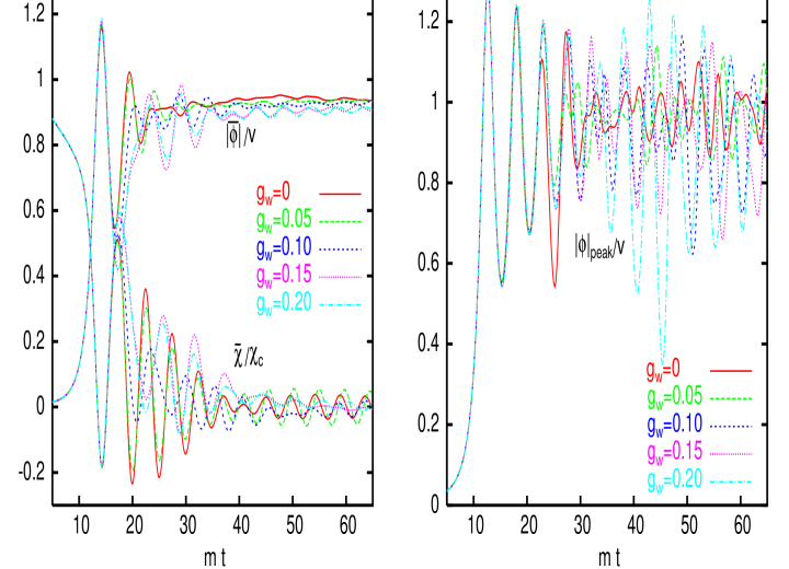
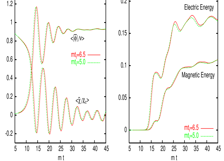
A first category of observables monitoring this process is given by the time evolution of the gauge invariant, spatial averages of and . In Fig. 1 (left) we show an illustration of such a time evolution for model A from the initial distribution at up to , where the system has stabilized around the true vacuum: the Higgs field gets close to its vacuum expectation value and the inflaton oscillates around zero with an amplitude that gets damped as time evolves. As mentioned previously the initial phases of this evolution involve the presence of Higgs boson lumps in space that grow with time. Figure 1 (right) shows the time evolution of the center of one of those lumps. Both the spatial averages and the value at the top of the lump are computed and shown for various values of the gauge coupling, including zero coupling. From the comparison it is clear that initially the dynamics is completely driven by the scalar sector of the model; only at later times, once the Higgs and inflaton fields have started oscillating around their vacuum expectation values, does the presence of gauge fields start to affect the evolution of these observables.
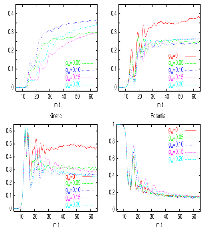
The moment in which the gauge fields start to play an essential role in the evolution is more clearly signaled by the time evolution of the total energy fractions. These quantities represent the relative contributions of the pure gauge electric and magnetic terms in the Hamiltonian, kinetic, gradient and potential terms of the Higgs and inflaton fields to the conserved total energy of the system. In Fig. 2 we display the electric plus magnetic energy fractions as a function of time for a given configuration in model A. The fast growth of the Higgs boson expectation value toward the true vacuum drives the growth of gauge fields, which start to contribute significantly after the mean value of the Higgs field has first reached the vacuum expectation value (compare with Fig. 1). Since the total energy is conserved during the evolution, the energy stored in the scalar fields decreases due to the nonzero gauge energy fraction. This affects mostly the kinetic and gradient energies of the scalar fields, while the potential energy remains essentially unaltered. This is also illustrated in Fig. 2, where we show the comparison of the average values of all energy fractions for various values of the gauge coupling. From the figure one notices a peculiar oscillatory dependence of the pure gauge energy fraction with respect to . We have actually analyzed this behavior in finer detail by running a few configurations for all values of from to in intervals of . The results will be commented upon later in Section IV-C, in relation to Chern-Simons production.
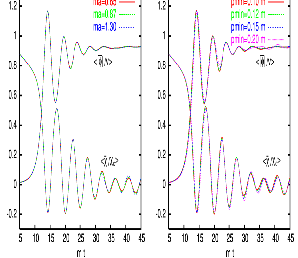
The previously discussed quantities provide an excellent testing ground for checking the independence of our results on the various cutoffs introduced in our procedure. As we discussed previously, the value of these cutoffs has to be chosen judiciously to guarantee the physical-character of the results. Figure 3 tests the dependence of the mean values of , , as well as electric and magnetic energies, on both and for model A1 (Table 1). The mean values result from averaging over space as well as over initial conditions. The dispersion over the different set of initial conditions gives rise to errors which are very small on the scale of the Figure. Up to we see no dependence at all of the evolution of the mean values on the ultraviolet cutoff. There is a slight dependence on the physical volume for , more significant for electric and magnetic energies than for , , but the results very rapidly converge as we increase the volume.
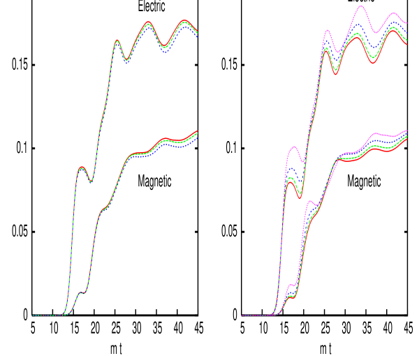
As in paper I we have also checked that our results do not depend strongly on the choice of the initial time at which the classical evolution starts. All the results presented in this paper correspond to the choice . In Fig. 4 we show a comparison of the evolution of spatial averages and the electric and magnetic gauge energy fractions for and (for model A1). Most of the difference can be compensated by an additional shift of size in time. It is clear that a change in is well accounted for by the change of initial conditions (very different in magnitude), chosen according to the quantum linear evolution. This proves the consistency of our analysis.
IV.2 Energy behavior and spectra
As discussed in Section III.1, the validity of the classical approximation rests on the fact that infrared modes dominate the dynamics of symmetry breaking and generation of Chern-Simons number. The reliability of this approximation during the relevant time scales has been challenged in Ref. moore . Moore has argued that, once gauge fields are coupled to the Higgs-inflaton system, it is the energy transfer between ultraviolet and infrared modes that drives the dynamics, long before the physically relevant processes have taken place. This would make it impossible to obtain a cutoff-independent description of the evolution of the system and would invalidate the use of the classical approximation. We will show in what follows that our results seem to be free of this criticism. Essential for this is our choice of initial conditions for the subsequent classical evolution. A similar conclusion was found in Ref. SST , which use analogous initial conditions.
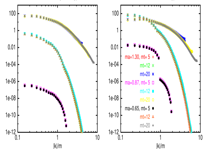
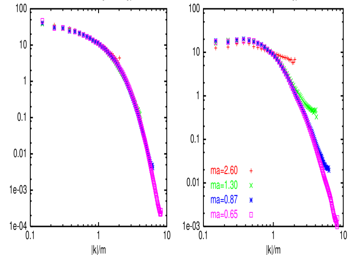
The crucial test to address Moore’s criticism is to check the independence of the results of the UV cutoff at all the relevant time scales. We have already tested this cutoff independence for average mean values and energies in the previous Section. Here we will extend the analysis to the Fourier spectra of the (gauge invariant) energy densities. This Fourier decomposition exposes in a more direct way the range of relevant momenta. Figure 5 shows, as an illustration, the time evolution of the spectra of the electric component of the gauge field energy density and of the Higgs-inflaton contribution to the potential energy density. A similar behavior is observed for the remaining terms (magnetic, kinetic, and gradient parts for the Higgs and inflaton fields) of the Hamiltonian. Results are presented for three different values of the lattice spacing: , , and . The results scale to an impressive degree, and only in the last stages of evolution do deviations start to be observed in the high momentum part of the distribution. In Fig. 6 we display the same Fourier spectra for . An enhancement of UV modes at the edge of the distribution is clearly observed. As time evolves this altered distribution affects lower-momentum modes as well, and tends to flatten the spectrum, creating an artificial thermalization of the system. This effect is already noticeable in the potential energy spectrum for , and only slightly in that of . Fortunately, as shown in Fig. 5, in our physically relevant time interval and for the actual values of the UV cutoff used in our analysis, we are free from this problem. As we will see in the next Section, the results on Chern-Simons number generation support this conclusion.
IV.3 Chern-Simons production
In this Section we will display our results concerning Chern-Simons number production. We measure the variation in Chern-Simons number between the initial time and a later time :
| (8) |
where the dual tensor is . Since our dynamics is CP conserving, the average value of over many configurations is zero. We can expect that the mechanism of Chern-Simons number production is local in space-time and characterized by a certain physical length scale. In such a situation it is more interesting to express the result in terms of the sphaleron rate , given by
| (9) |
which is independent of the physical volume of the system. The symbol denotes the expectation value with respect to configurations obtained with different initial conditions (i.e. different random realizations). The factor is introduced to make dimensionless. In our nonstationary situation, in which the sphaleron rate might be time dependent, it is better to display the quantity:
| (10) |
Our lattice implementation of the topological charge density is based on the discretized definitions of the electric and magnetic fields in terms of temporal and spatial plaquettes, respectively. We have used , (for the electric field) and (for the magnetic field) plaquettes combined in such a way as to subtract the leading correction for smooth fields. As we will see, our gauge fields vary over scales of the order of , which extend over several lattice spacings. Our improved discretization of the topological charge density guarantees that we do not introduce additional corrections in our Chern-Simons measurement. The situation contrasts with the one encountered in measurements of the sphaleron rate at thermal equilibrium, where modes of the order of the cutoff are excited. We address the reader to the extensive literature on the subject sphalrate .
As we will show later in this Section, in contrast to other quantities described in the previous Subsections, the Chern-Simons number fluctuates considerably from configuration to configuration. It behaves like a random variable with a fairly large dispersion value. Thus, to give a sufficiently precise value of , one has to generate and average over many configurations. The required precision is partly determined by the possibility of testing the cutoff independence of the results. Concerning the latter issue it was established in previous Sections that there is a window of values of and where the dynamics of the system is insensitive to the actual values of these cutoffs. However, the Chern-Simons number might be more sensitive to a scale on which cutoff effects are more apparent.
Although the Chern-Simons production mechanism is expected to be quite different from the typical sphaleron tunneling processes in the vacuum, it is still natural to expect that the relevant scales involved are of the order of the two physical scales given by the Higgs and W boson masses (, ). Thus, insensitivity to the ultraviolet cutoff demands that and be small. The first requirement is hard to meet with our present limitations of computer memory and power. To reach values of , while keeping the ultraviolet and infrared effects under control, would require and , which implies large lattices, . With our present capabilities, we can reach values of that are only slightly below unity. Reducing this value compromises the volume independence of the dynamics, since the physical size of the bubbles become comparable to our physical box size. Fortunately, we know that in the low-temperature tunneling process between different vacua, sphalerons exist in the limit . Thus, in this case the only relevant cutoff-dependent parameter is , which can be made small by tuning the gauge coupling and . This situation was indeed confirmed by previous lattice studies of sphalerons margapierre . Our choice of ultraviolet and infrared cutoff values will be made within the region that was found adequate in that study: the range given by , for to , for , where is the linear extent of the lattice in physical units. As we will see, our results confirm that this is also the case in our situation.
In conclusion, in order to study the physical Chern-Simons production in our dynamical process, we have considered several models having different degrees of sensitivity to cutoff effects. The most favorable case, model A1, on which most of our study was focused, has and , giving . The purpose of studying other models is two-fold. On one hand we can test the sensitivity of the production mechanism to the ratio of scales , as was done recently for the Abelian case ST . On the other hand, our study is meant to be a pilot one, which will allow the determination of the computer resource requirements for the study of other specific models. For the different models (see Table 1), volumes and lattice spacings we have generated typically configurations on which our results are based. The full list of models, cutoff values, and the exact number of configurations on which our results are based are collected in Table 2. As explained before, the linear size of our box, in units, is determined by the value of , by the expression . On the other hand, the value of the lattice spacing in physical units is determined by the number of lattice points in each direction , by the formula . This allows us to test ultraviolet and infrared effects separately by changing these two quantities ( and ) independently.
| Model | Confs. | ||||||||
|---|---|---|---|---|---|---|---|---|---|
| A1 | 64 | 0.12 | 134 | 3.24(0.36) | 7.94(0.87) | 8.22(0.88) | 12.35(1.25) | 13.77(1.49) | 12.45(2.00) |
| A1 | 48 | 0.12 | 191 | 3.77(0.35) | 7.59(0.72) | 7.72(0.80) | 10.52(1.02) | 12.12(1.08) | 11.98(1.06) |
| A1 | 64 | 0.15 | 140 | 4.14(0.42) | 9.39(1.05) | 9.20(0.99) | 11.41(1.25) | 12.92(1.40) | 13.47(1.45) |
| A1 | 48 | 0.15 | 191 | 4.35(0.43) | 7.97(0.80) | 7.46(0.48) | 10.55(1.02) | 12.76(1.22) | 11.22(1.25) |
| A1 | 32 | 0.15 | 167 | 4.61(0.56) | 8.60(0.94) | 8.54(0.72) | 10.50(1.13) | 11.85(1.26) | 11.37(0.95) |
| A1 | 48 | 0.2 | 152 | 5.91(0.49) | 6.36(0.64) | 6.82(0.37) | 8.92(0.91) | 9.32(0.99) | 9.47(1.21) |
| B | 48 | 0.12 | 188 | 6.27(0.74) | 12.49(1.41) | 10.81(1.03) | 13.86(1.54) | 17.19(1.99) | 14.70(1.47) |
| B | 64 | 0.15 | 182 | 8.10(0.92) | 13.86(1.22) | 15.16(2.26) | 17.16(1.45) | 19.89(1.74) | 19.60(3.26) |
| B | 48 | 0.15 | 200 | 7.46(0.80) | 12.77(1.33) | 11.65(1.23) | 14.74(1.39) | 17.79(1.68) | 15.11(1.67) |
| B | 32 | 0.15 | 170 | 8.26(0.92) | 10.83(1.19) | 7.93(0.98) | 13.29(1.46) | 14.89(1.65) | 10.84(1.31) |
| A2 | 48 | 0.15 | 210 | 5.41(0.60) | 17.63(1.62) | 17.39(1.22) | 25.16(2.54) | 33.87(3.61) | 24.79(2.20) |
| A3 | 48 | 0.15 | 128 | 3.52(0.41) | 19.46(2.67) | 14.72(1.50) | 28.71(4.25) | 38.00(5.62) | 26.22(2.68) |
| A3 | 32 | 0.15 | 181 | 3.58(0.42) | 14.68(1.64) | 12.85(1.35) | 20.80(2.08) | 24.58(2.42) | 22.92(2.02) |
| A4 | 48 | 0.15 | 157 | 0.54(0.06) | 5.06(0.52) | 4.72(0.41) | 10.03(1.07) | 16.10(1.74) | 14.69(1.49) |
| A4 | 32 | 0.15 | 181 | 0.70(0.06) | 6.49(0.72) | 5.56(0.43) | 10.12(1.00) | 14.17(1.44) | 13.71(1.44) |
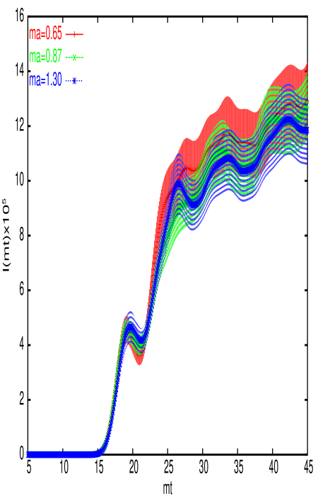
We stress that volume and lattice-spacing dependences should affect the data very differently. The distribution of Chern-Simons number should not depend on the value of if ultraviolet cutoff effects are small. This is very well satisfied by our data on as seen in Fig. 7, where we have displayed the time evolution of this quantity for model A1, and various values of the ultraviolet cutoff (), (), and (). In this figure we observe that starts growing from zero, its initial value, at a time . This growth is very steep and presents oscillations up to a value of . Then the growth continues with a smaller slope. The insensitivity of our results to the value of the ultraviolet cutoff is very striking given the relatively large value of . It provides evidence that the relevant cutoff scale is (=, , ).
If the mechanism of Chern-Simons generation is local in space, one expects that a change in the volume should modify the dispersion proportionally. Therefore, as mentioned previously, the quantities and should be independent of the spatial volume.
Our results for at various times ( and ) are collected in Table 2. The errors quoted within parentheses are computed in the standard fashion from the dispersion within the various configurations. For a typical number of configurations of approximately 150, they are around 10. For model A1 the results for various volumes are displayed, showing a large degree of independence of of . There is nevertheless some significant dependence for the smallest volume (). This dependence was also observed in mean values and energies. For all the quantities the volume dependence decreases considerably for larger volumes (), being of the order of the quoted errors.
Furthermore, the cutoff independence of the data is an important and nontrivial point. Choosing values of the model parameters outside the relatively small optimal range gives results that behave quite differently (e.g., rising with ). The fluctuating nature of forces one to accumulate a certain amount of data before the cutoff dependence shows up clearly. This sends a word of warning to other researchers studying similar questions.
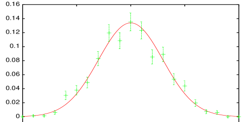
In addition to studying the value and time dependence of , it is interesting to investigate the distribution of values of the Chern-Simons number for various times. In the absence of a CP violating term this distribution should be centered at and have a dispersion determined by the value of . Assuming, as we did before, that the Chern-Simons number is produced in local structures with arbitrary signs, one expects the distribution to be of the Poisson type. This, for large number of structures, is close to a Gaussian distribution centered at zero. Indeed, our results agree with these expectations. Histogramming, normalizing and fitting the data to a Gaussian allows one to obtain an estimate of , the only parameter of the fit. The values for and are displayed in Table 2 (using the symbol . The resulting per degree of freedom was most of the time of the order of 1 and never larger than 2. This confirms that the distribution of the Chern-Simons number over the different configurations is compatible with a Gaussian. In Fig. 8 we show a combined histogram of our data for model A1, , , and all values of . The normalized Gaussian that best fits the data is also displayed. The of the fit is per degree of freedom, and the value of resulting from the fit is , which is perfectly compatible with the data in Table 2.
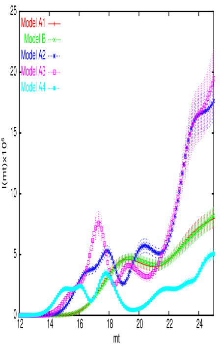
Finally, we will comment on the results for other values of the parameters of the model. It is obvious from Table 2 that the results are of the same order of magnitude, but might differ by factors of 2 or larger. In order to make a direct comparison one should take into account that the time evolution of is quite different for all the models. This is shown in Fig. 9 where we display for and for all the models and a relevant range of times. The data corresponding to model B are shifted in time by and scaled up by . With this modification they match perfectly with those of model A1. These two models have a common value of . We find this agreement remarkable, since model B is in a region of parameters that is expected to be more sensitive to ultraviolet and infrared cutoffs. On the other hand all A-models have the same value of and different values of , and hence different ratio of masses. It is clear that the evolution of has a fairly sensitive dependence on . A similar strong dependence of the Chern-Simons number on has been reported recently for the (1+1)-dimensional Abelian model ST . We found a certain positive correlation between the values of the gauge-energy fraction and that of . Since the former quantity has fewer fluctuations and requires fewer statistics, we studied a few configurations for all values of ranging from up to in intervals of and monitored the fraction of gauge energy at . The result shows an oscillation, growing from to a maximum at (model A2), and then decreasing up to , where it begins to grow again. We therefore expect that the maximum values of attainable in this region of parameters are not far from those of model A2.
IV.4 Space-time structures
In this Subsection we will investigate the local structures associated with Chern-Simons number production. Since in the first stages of evolution and for our choice of inflaton coupling (), the Higgs and the inflaton fields evolve collinearly, we will restrict our analysis to Higgs and gauge field structures.
Initially the space-time structures of the scalar fields do not differ significantly from those of paper I, in which gauge fields are decoupled. Snapshots of the evolution of the Higgs field from the growth of spatial lumps to the generation of bubbles were presented there, where we also gave a partial analytical description of the process.
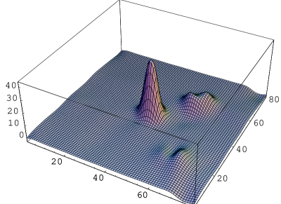
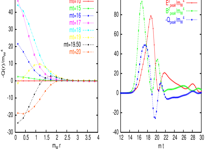
Our main interest now concerns the structure of the topological charge density , which integrated over space and time gives rise to , as described in the previous Section. For the case of model A1, starts to become sizable at . The local origin of this growth is well exemplified by the snapshots of on two dimensional slices presented in Fig. 10. The slices were chosen to coincide in one coordinate with a local maximum of the topological charge density. Lumps such as the ones observed in the figure become manifest for . During the following stages of evolution, their position remains unchanged but the value at the peak presents an oscillatory pattern, as was the case for the Higgs boson lumps, even flipping the sign of the charge density at the center of the lump. This is illustrated in Fig. 11 (left) where the charge density profile is shown at different times for the same configuration displayed in Fig. 10. The origin of this oscillation seems to be associated to a similar oscillatory behavior of the electric and magnetic fields. This can be deduced from their behavior at the center of the charge density peak as a function of time which is displayed in Fig. 11 (right). Electric and magnetic fields oscillate out of phase, and changes in the sign of the charge density seem to take place when the modulus of either the magnetic or the electric field vanishes. The flip of sign of the charge density could be a possible explanation for the oscillation in observed around in Fig. 7.
To provide a more systematic statistical study of the local structure of the topological charge density, we have performed a detailed study of a few configurations of model A1 with and . The data show a remarkable spatial concentration of the density. For example, selecting the lattice points () for which , we find that they occupy only a few percent of the lattice volume (, and for , , and , respectively), while they account for a large fraction of the total charge squared (, , and ).
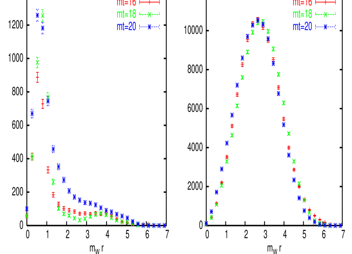
Another way to investigate clustering is by identifying local maxima (or “peaks”) of the distribution , with height above a certain threshold (). The number of these peaks starts to be nonzero for , about the time when we start to observe a fast growth in the dispersion of the Chern-Simons number. Beyond this time, and up to , there are typically a few ( ) such maxima. Most of the points in are clustered around these peaks, as shown by the histogram of minimum distances from points in to the peaks Fig. 12 (right). The shape has to be compared with the histogram of minimum distance from any lattice point to one of the peaks, which gives a measure of phase-space, see Fig. 12 (left). From the comparison one also concludes that the majority of points which are sufficiently close to one of the peaks belong to . Thus, peaks identify structures of the size of a few lattice spacings, compatible with in physical units.
A similar conclusion can be drawn by computing the fraction of charge density square contained inside spheres of radius around each peak. This amounts to , and at , , and respectively, while these spheres occupy only , , and of the total lattice volume. Summarizing, we conclude from the results of this analysis, that the topological charge density is concentrated in local structures of typical size , such as those depicted in Fig. 10. Similar structures are also observed in the electric and magnetic energy densities.
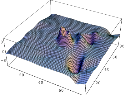
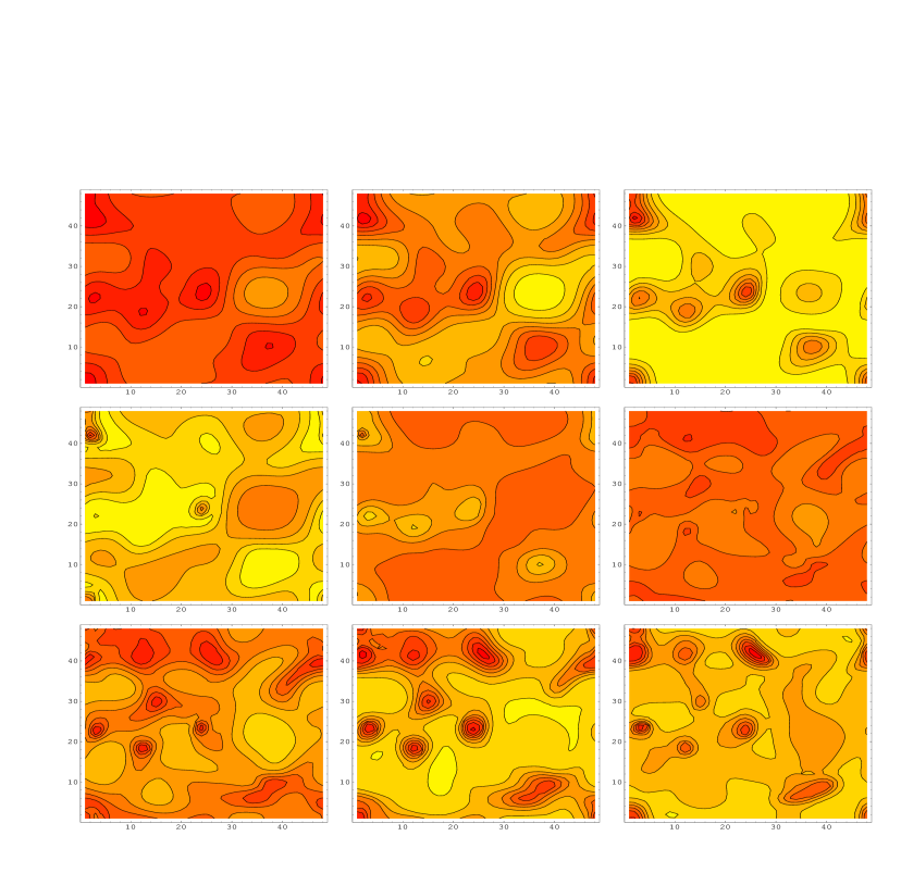
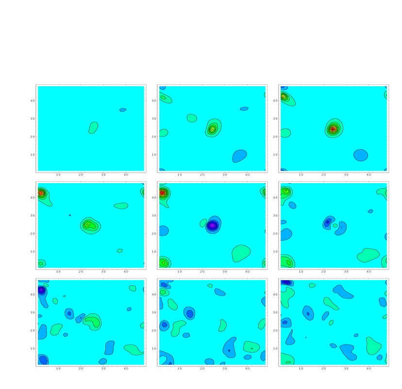
In view of these results one might be tempted to identify the local structures appearing in the first stages of evolution with sphaleronlike configurations KM . Sphalerons are static solutions of the SU(2)-Higgs classical equations of motion with fractional Chern-Simons number. They have indeed a localized, lumpy, energy density with a typical size given by . However, it is essential for the sphalerons that lumps in the energy density are correlated with zeros in the Higgs field, i.e. gets a maximum at the location where . To take a closer look at the correlation between the structures of the Higgs field and of the topological charge density in our configurations, we present in Figs. 13 and 14 contour plots of and on two-dimensional slices for various values of .
Let us first analyze the Higgs contours on Fig. 13. Contours are shaded such that the false vacuum () is represented by red (dark in black and white display), while the true vacuum () is yellow (light in black and white display). At we observe the formation of the first Higgs lumps [medium grey (orange) in the figure], which grow from local maxima in the initial random Gaussian distribution of the Higgs field. These lumps grow, reach the minimum of the potential, and start to oscillate around it; see , , and . As observed in Fig. 13 there are a series of very localized regions between lumps which remain in the false vacuum [dark (red)] for a longer time and only much later start to oscillate around the minimum of the potential, almost opposite in phase to the oscillations of the Higgs homogeneous zero mode footnote . Remarkably, it is precisely at these points where localized lumps appear in the topological charge density, appearing as red regions (dark in black ¿ and white display) in Fig. 14. Notice, however, that there is a relative time shift between the presence of zeroes in the Higgs field and that of maxima in the charge density.
In summary, we have shown that there is a clear association between the behavior of and the presence of local structures of size in gauge degrees of freedom, also correlated to certain structures in the Higgs field. A more detailed investigation of these issues is certainly interesting but demands more intensive studies which fall beyond the scope of this paper.
V Baryogenesis
In this Section we will illustrate how the results of the previous ones can be related to baryon number generation. In the Standard Model, baryon and lepton numbers are not conserved because of the anomalous nonconservation of the associated left-handed fermionic (leptonic or baryonic) currents, , through the chiral anomaly tHooft ,
| (11) |
where is the topological charge density studied in the previous Section, and is the Chern-Simons current. In this way we see how the change in baryon and lepton numbers are related to that of the Chern-Simons number: .
At zero temperature variations in Chern-Simons number can proceed through a tunneling process tHooft with negligible probabilities . We will refer to those transitions (quantum or classical) that change Chern-Simons number as sphaleron transitions.
At nonzero temperatures thermal fluctuations can help the generation of hot sphalerons, allowing over-the-barrier transitions between different vacua that may be responsible for baryon production KRS . Below the critical temperature they are still exponentially suppressed, but with a temperature-dependent rate, , where is the sphaleron energy. However, at high temperatures, the sphaleron transitions are mainly sensitive to the long-wavelength modes in the hot plasma. A simple argument then suggests that the rate of sphaleron transitions per unit time per unit volume should be of the order of the fourth power of the magnetic screening length in the plasma armcl ; khsh .
Away from equilibrium the transition rate is harder to estimate. However, in Ref. GGKS it was proposed that the sphaleron transition rate during rescattering after preheating, , could be high, and could be estimated as that of a system in local thermal equilibrium at some effective temperature for the long-wave modes, , characteristic of the equipartition energy stored in those modes, .
The absence of a CP-violating interaction in our model implies that the average value of must be zero and no net baryon number can be created on the average. However, there is a scenario for incorporating a CP-violating effect proposed in Ref. GGKS , which will allow us to connect the results presented in the previous Sections with the issue of EW baryogenesis. This will be explained in what follows.
One possible way to induce a CP-asymmetry within the effective field theory approach, is to consider the inclusion of nonrenormalizable operators that violate CP. These could be low energy remnants of additional degrees of freedom and interactions present at a higher energy scale . The lowest dimension-6 operator of this sort is misha
| (12) |
which is both P and CP violating. The dimensionless parameter is then an effective measure of CP violation. The factor is introduced in order to simplify the subsequent formulas. Note that the operator (12) does not violate C, and therefore in the bosonic sector of the theory the nonequilibrium evolution can produce only P- and CP-odd configurations. The required C violation comes from the fermionic sector of the theory, which has not been included in our work. These C-violating operators appear in gauge-fermion EW interactions that violate C and P, but conserve CP.
Following Ref. GGKS , we will assume that the operator (12) induces an effective chemical potential , which introduces a bias, i.e. a slope, in the potential of EW vacua, between baryons and antibaryons GGKS ,
| (13) |
Although the system is very far from thermal equilibrium, we will assume that the collision integral equation governing the time evolution of the baryon number density can be cast in the form of a Boltzmann-like equation, where only the long-wavelength modes contribute misha ; GGKS
| (14) |
where is the time-dependent effective chemical potential (13), and is the term responsible for baryon washout khsh . As can be deduced from Fig. 7, the sphaleron rate grows very quickly initially but then decreases to a much lower value at later times. On the other hand, the effective temperature decreases because of rescattering, while the energy stored in the long-wave modes is transferred to the high-momentum modes GGKS ; FK ; GBKLT . The washout rate is smaller, even at high temperatures, than the other scales. For instance, for GeV and we obtain GeV, which is small compared with the tachyonic Higgs growth toward symmetry breaking ( GeV). It is also much smaller than the perturbative decay rates of the Higgs boson into gauge fields, or those into light fermions. Therefore, we will assume that the last term in Eq. (14) is negligible during baryon production immediately after EW symmetry breaking, and the final baryon asymmetry can thus be estimated by integrating Eq. (14):
| (15) |
where all quantities are evaluated at the time of symmetry breaking (more precisely at the maximum of the sphaleron rate). This corresponds to a baryon asymmetry
| (16) |
where is the number of effective degrees of freedom that contribute to the entropy density, , at the electroweak scale. Taking the scale of new physics to be at TeV, the Higgs boson mass GeV, the sphaleron rate (see Table 2), and the effective temperature GeV, we find
| (17) |
consistent with observations for , a perfectly acceptable value for particle physics beyond the standard model. Therefore, baryogenesis at EW preheating after hybrid inflation GGKS can be very efficient, in the presence of a new source of CP violation. Varying the scale of the new physics , one can satisfy the observational constraints by changing accordingly.
The previous calculation has to be understood as an order of magnitude estimation of the baryon number production within the scenario of Ref. GGKS , since there are clear uncertainties in both (with realistic couplings) and . Furthermore, there are also theoretical caveats. On one hand, the connection between Chern-Simons number and baryon number generation in a nonperturbative setting as ours has been questioned in Ref. klinkhamer . On the other hand, doubts have also been expressed in Ref. RSC about the validity of the Boltzmann equation (15) in a non-Markovian evolution of the Chern-Simons number production. Modulo these warnings, we may conclude that the observed baryon asymmetry does not require unnaturally large values of . Remarkably, a recent paper ST2 that does include the CP-violating operator (12) in the simulations finds a similar estimate of the baryon number generated within this scenario, despite the use of different initial conditions (quench approximation, etc.) and model parameters.
VI Conclusions
In this paper we have studied the evolution with time of a quantum field theory containing the SU(2) gauge-scalar sector of the standard model coupled to a singlet inflaton. The initial state of the system follows from the end of a hybrid inflation scenario, which is dominated by a slowly decreasing homogeneous inflaton mode, coupled to Higgs and gauge fields in the Minkowski vacuum. The tachyonic instability of the model at the initial stages triggers the fast growth of the infrared modes of the Higgs, which evolve toward classical behavior. This provides justification of our main approximation: the assumption that the classical evolution of this field leads to a classical behavior of the remaining modes of the whole system, and that this occurs before the nonlinear effects, including backreaction become important. The consistency and justification of this idea were studied in paper I, in the absence of gauge fields. Other authors have applied similar ideas PS ; TK ; GBKLT ; CPR in different contexts. In this paper, we built upon this idea and incorporated gauge fields in the problem. We have tested the self-consistency of the scheme by varying the initial time for the classical evolution of the system , with the corresponding change in the distribution of random initial conditions (changing by orders of magnitude), as determined by the quantum linear evolution of the Higgs modes. Our results are robust to these changes, as well as to the specific details in which the initial conditions of the gauge fields are introduced.
We have studied the classical evolution of the system using lattice methods for a variety of model parameters. Their choice has been done judiciously to minimize the effect of the ultraviolet and infrared cutoffs. The resulting time evolution of global quantitiesmean values of the Higgs and inflaton fields, energy fractions, etc.is fairly insensitive to the randomly chosen (with a fixed distribution) initial condition. It is also insensitive to the value of the ultraviolet and infrared cutoffs, if chosen in the appropriate range. This is confirmed by the shape of the spectral distribution of the gauge and Higgs fields. The dynamics is dominated by the modes lying far from the edges, where cutoff effects are dominant. Therefore, the results in this region of time seem free of the concerns expressed by Moore moore .
The main part of our work has focused on the study of the evolution of Chern-Simons number with time. This turns out to be a much more fluctuating quantity than the aforementioned average values. This has forced us to accumulate a considerable amount of statistics in order to draw conclusive results. Finally, our results provide evidence that the dynamics of the system leads to the generation of Chern-Simons number, a prerequisite for it to lead to baryon number generation. The mechanism for this generation is found to be local and stochastic.
In conclusion, our work provides a step toward the study of a new mechanism for baryogenesis based on the out of equilibrium situation occurring during the preheating stage in hybrid inflation scenario GGKS . There is still a long way to go before this idea can turn into a full-scale proposal for baryogenesis at the electroweak scale. Perhaps the most important new ingredient required is the incorporation of a CP-violating term which would translate the generation of Chern-Simons number into an actual baryon number at the required rate. We have assumed in Sect. V a concrete CP-violating operator which is proportional to the baryonic current and thus induces a chemical potential for the baryon number GGKS , biasing sphaleron transitions toward baryons rather than antibaryons. In that case, it seems possible to reproduce the observed baryon asymmetry of the Universe with a reasonable amplitude of the CP-violating interaction, in the context of sphaleron transitions at EW symmetry breaking, i.e. during tachyonic preheating after hybrid inflation.
Acknowledgements
It is a pleasure to thank E. Copeland, D. Grigoriev, F. Klinkhamer, A. Kusenko, G. Moore, A. Rajantie, P. Saffin, M. Shaposhnikov, J. Smit, and A. Tranberg for useful comments, suggestions and constructive criticism. This work was supported in part by a CICYT project FPA2000-980.
Appendix A The Lattice Equations of Motion
In this appendix we explain in full detail the derivation of the lattice equations of motion. We start by fixing our conventions. Let us denote the lattice by . The lattice points are labeled , whose corresponding space-time position is , where and are the temporal and spatial lattice spacings. The ratio of spacings will be called . The lattice inflaton and Higgs fields are and . They are dimensionless and correspond to the product of the continuum fields by the lattice spacing . Gauge fields are given by link variables , which are SU(2) matrices. Therefore, both the gauge and Higgs fields are described by matrices of a certain type. If we choose the matrices as a basis of the space of complex matrices ( are the Pauli matrices), we might decompose the lattice Higgs field as follows:
| (18) |
where the coefficients are real. Matrices of this type are closed under addition and multiplication. They form a field , which is isomorphic to the field of quaternions. The link variables are also members of this space:
| (19) |
where the coefficients are real and define, for every direction and lattice point, a vector of unit modulus:
| (20) |
An arbitrary matrix belonging to satisfies the following relations:
| (21) | |||||
| (22) |
where stands for equality up to a multiple of the unit matrix. We will make use of the previous relations extensively in the following.
A lattice gauge transformation is given by a collection of SU(2) matrices, one for every point of space . The fields transform as follows:
| (23) | |||||
| (24) |
where is the unit vector in the direction. We will also be concerned about composite lattice fields defined on plaquettes:
| (25) |
which transform as
| (26) |
It will be convenient to introduce lattice covariant derivatives . The lattice covariant derivative is different for fields transforming differently under gauge transformations. However, for ease of notation we will use the same symbol for all types of fields. In any case, the covariant derivative of a field transforms like the field itself. For a Higgs field the covariant derivative is given by
| (27) |
For a link variable and a plaquette variable the covariant derivatives are given by
| (28) | |||
| (29) |
For vanishing gauge fields the lattice covariant derivative reduces to the forward difference operator :
| (30) |
We will also need an adjoint covariant derivative operator reducing to the backward difference operator :
| (31) |
For a Higgs field one has
| (32) |
The reader can easily work out the corresponding definitions for link and plaquette fields.
A final notational convention will help us simplify the lattice formulas. We will introduce a lattice metric tensor which can be used to raise four-dimensional indices in the standard way. The tensor is diagonal and its components are , . This will allow us to use a restricted Einstein summation convention: Except when explicitly specified, summation is implied whenever a term contains an upper and a lower space-time index which are identical.
We are now ready to introduce the dynamics of the fields. This is given by the lattice action :
| (33) | |||||
The Lagrangian has been split into four parts. contains the pure gauge interaction, and are the (kinetic) part of the total Lagrangian containing space-time (covariant) derivatives of the Higgs and inflaton fields, respectively; finally, the potential contains only point-like interactions of these fields. The explicit forms of the different Lagrangian terms that we are using are
| (34) | |||||
| (35) | |||||
| (36) | |||||
| (37) | |||||
where we have used the lattice metric tensor to raise indices. All terms are obviously gauge invariant. The constants and appearing in the potential are the same couplings that appear in the continuum Lagrangian. The dimensionless lattice mass terms and are the product of the continuum mass terms by the lattice spacing (, ).
To derive the equations of motion one has to impose that the derivative of the action with respect to each of the fields vanishes. Let us begin with the inflaton field . Only the third and fourth terms in the Lagrangian depend on this field. After straightforward operations, one obtains
| (38) |
Similarly the equation for the Higgs field can be deduced. In matrix notation the equation reads:
| (39) |
In our notation, both equations are very similar to their continuum counterparts [see Eq. (3].
The derivation of the equation of motion for the gauge field is a bit more tricky. We can deduce it by equating to zero the derivatives of with respect to the real coefficients , appearing in Eq. (19). However, the coefficients are not independent, since they are subject to the constraint Eq. (20). This can be taken into account by using Lagrange multipliers. Hence, the equation of motion for the gauge field has the form
| (40) |
where the coefficients are Lagrange multiplier fields, which are determined by the condition that the evolution preserves the constraint Eq. (20). To work out the first term in Eq. (40), it is convenient to express as follows:
| (41) |
where is given by the standard sum over staples, and the ellipsis represents terms that do not depend on . Then, one can reexpress the gauge field evolution equation as (no summation on on the right hand side)
| (42) |
where all three terms transform in the same way (as a link variable) under gauge transformations. The are not necessarily the same as the multipliers, but this will be irrelevant in the following. The explicit expressions for and are
| (43) | |||||
| (44) |
Despite the simple expression of our gauge field evolution equation (42), it is convenient to transform it into a form which more closely resembles the continuum equations of motion. For that purpose, we multiply the equation by and obtain
| (45) |
where no summation over is implied, and the equality holds modulo a multiple of the identity matrix. To turn it into an exact identity we might simply add up the traceless part of the two terms on the left hand side. For a matrix belonging to , the traceless part is simply . Hence, let us introduce the following traceless matrices:
| (46) | |||||
| (47) |
where again no summation is implied. The equation of motion for the gauge fields then reads:
| (48) |
The second term in this equation is the lattice version of the current. Manipulating Eq. (46) one can rewrite it in a way completely analogous to the continuum case:
| (49) |
To cast Eq. (47) in a way similar to the continuum expression [Eq. (3) of Sect. III] we introduce the lattice counterpart of the field strength:
| (50) |
The gauge equation of motion can finally be written as
| (51) |
In all the previous derivation we have worked in an arbitrary gauge. However, to have a uniquely defined initial value problem in order to solve the equations numerically, it is convenient to fix the temporal gauge,
| (52) |
The lattice equations of motion can now be used to express the value of the fields at time in terms of the fields at time and . By using these relations iteratively, one achieves the numerical evolution of the system. However, although the temporal component of the gauge potential has been set to zero, the corresponding equation of motion is still present. This is precisely Gauss’s law:
| (53) |
This equation is of a different nature than the other ones, since it relates the field values at times and : It is a constraint on the initial value data. Indeed, in the continuum we know that the constraint is conserved through the evolution equations, so that if it is satisfied at one time, it is satisfied at all times. Our next goal will be to show that this is also the case on the lattice.
To study the time variation of Gauss’s law, we apply the operator to both sides of Eq. (53). Using the equation of motion for the Higgs field one obtains
| (54) |
which is the lattice counterpart of the continuity equation.
Now we should study the action of the lattice backward time difference operator on the left hand side of Eq. (53). The essential property that will be needed in the proof is:
| (55) |
where there is no summation implied on either or . This expresses the commutativity of the covariant derivatives when acting on the field strength. In general, however, the covariant derivatives do not commute. Given this commutativity, we obtain the following chain of equalities:
| (56) | |||||
In the first equality we used the commutativity, in the second the gauge field equations of motion, and in the third we used the commutativity again together with the antisymmetry of the field tensor. Notice that there is now an implicit summation over and .
In summary, we have showed that both sides of Gauss’s law vary in the same way with time. This implies not only that fields satisfying Gauss’s law initially will satisfy it at later times, but also that any initial deviation will remain constant with time. Altogether, the conclusion is based on the consistency of the gauge field equations with the covariant conservation of the current, which relies on
| (57) |
where now summation is implied.
Appendix B The Gauss Constraint
In this appendix we will explain in detail how we have implemented the Gauss constraint on the initial conditions for the Higgs and gauge fields. The procedure that we have used in practice is very similar to the one adopted in ST for Abelian gauge fields.
The Gauss constraint relates the electric component of the gauge field to the current. Thus, our criterion, in agreement with the considerations made in Sect. III.2.1, has been to fix the initial (at ) magnetic field to zero. This allows us to fix the gauge in such a way that the initial vector potential is zero, but with a nonzero time derivative, i.e. a nonzero electric field strength. The resulting form of the Gauss constraint equation in the gauge is the same as in the Abelian case, , where is the charge density generated by the Higgs field. A necessary condition for this equation to have a solution is that the total charge vanishes, i.e. . This condition is automatically satisfied with our particular choice of initial conditions for the Higgs fields, since with a real color-independent constant. To obtain a unique solution we can impose the requirement that the transverse components of the initial electric field vanish. This amounts to imposing the condition that not only the magnetic field, but also its time derivative vanishes at . With this choice we obtain the solution of the Gauss constraint in Fourier space, given by for and .
The previous construction can easily be translated to the lattice. The spatial links at the initial time are set to unity, and the links at the next temporal slice are obtained as , where the Fourier components of follow a formula equivalent to that of the continuum. This provides a solution to the lattice Gauss constraint up to terms of order , which, due to the smallness of the initial gauge field, are zero to machine precision. As mentioned before, due to rounding errors, small violations of the Gauss constraint at later times are induced during the numerical integration of the equations of motion. However, within the time scales we have analyzed they remain smaller than .
The strategy followed in our implementation of the Gauss constraint has been to avoid modifications in the initial distribution of the Higgs field. However, there are alternative approaches that, within a similar spirit, allow us to check the robustness of our choice. In particular, we could set to zero both the initial electric and magnetic fields and allow for minimal modifications of the Higgs field that preserve and . For the Gauss constraint to be satisfied in that case, the Higgs field has to be adjusted such as to have local zero charge density: . A particular solution is to take . Figure 15 compares the spatial averages of , , and the electric and magnetic average energy fractions thus obtained with the ones derived with our standard procedure. The results correspond to two configurations with the same initial distribution for the Higgs field up to the modifications induced by the two different ways of imposing the Gauss constraint. As can be observed the results are rather insensitive to the particular choice of initial conditions. The differences observed are quantitatively similar to the ones obtained from different realizations of the random Gaussian initial conditions for the Higgs field.
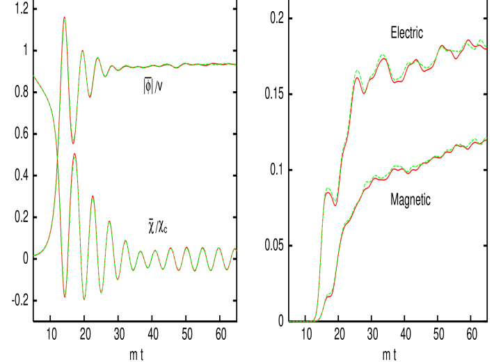
References
- (1) A. D. Sakharov, JETP Lett. 6, 24 (1967).
- (2) For a review, see V. A. Rubakov and M. E. Shaposhnikov, Phys. Usp. 39, 461 (1996).
- (3) V.A. Kuzmin, V.A. Rubakov, and M.E. Shaposhnikov, Phys. Lett. B155, 36 (1985).
- (4) K. Rummukainen, M. Tsypin, K. Kajantie, M. Laine and M. E. Shaposhnikov, Nucl. Phys. B532, 283 (1998).
- (5) Particle Data Group, http://pdg.web.cern.ch
- (6) An alternative proposal is that of leptogenesis [M. Fukugita and T. Yanagida, Phys. Lett. B 174, 45 (1986)], which may have occurred via a lepton asymmetry at much higher energies that was later converted into a baryon asymmetry through nonperturbative sphaleron processes above the electroweak scale.
- (7) L. Kofman, A. Linde and A. A. Starobinsky, Phys. Rev. Lett. 73, 3195 (1994); Phys. Rev. D 56, 3258 (1997).
- (8) L. Kofman, A. Linde and A. A. Starobinsky, Phys. Rev. Lett. 76, 1011 (1996); I.I. Tkachev, Phys. Lett. B 376, 35 (1996).
- (9) J. García-Bellido, D. Grigoriev, A. Kusenko and M. Shaposhnikov, Phys. Rev. D 60, 123504 (1999).
- (10) L. M. Krauss and M. Trodden, Phys. Rev. Lett. 83, 1502 (1999).
- (11) J. García-Bellido and D. Grigoriev, J. High Energy Phys. 01, 017 (2000).
- (12) D. Grigoriev, “Electroweak Baryogenesis at and after Preheating: What’s the difference?”, in the proceedings of the 35th Rencontres de Moriond: Electroweak Interactions and Unified Theories, E-print archive: hep-ph/0006115 (2000). J. García-Bellido, “Electroweak Baryogenesis from Preheating”, in the Proceedings of COSMO-99, hep-ph/0002256.
- (13) J. M. Cornwall and A. Kusenko, Phys. Rev. D 61, 103510 (2000); J. M. Cornwall, D. Grigoriev and A. Kusenko, Phys. Rev. D 64, 123518 (2001).
-
(14)
J. García-Bellido, “Particle Production and
Symmetry Breaking after Hybrid Inflation”, Plenary talk at
COSMO-01, International Workshop on Particle Physics and the Early
Universe, 2001, Rovaniemi, Finland. For a
transcript of the talk see
http://www.physics.helsinki.fi/cosmo_01/friday/Garcia-Bellido.pdf - (15) D. Lyth, Phys. Lett. B 466, 85 (1999).
- (16) N. Arkani-Hamed, H. C. Cheng, P. Creminelli and L. Randall, “Extranatural inflation,” Phys. Rev. Lett. 90, 221302 (2003); “Pseudonatural inflation,” hep-th/0302034; D. E. Kaplan and N. J. Weiner, “Little Inflatons and Gauge Inflation,” hep-ph/0302014.
- (17) G. Felder, J. García-Bellido, P. Greene, L. Kofman, A. D. Linde, and I. Tkachev, Phys. Rev. Lett. 87, 011601 (2001); G. Felder, L. Kofman and A. D. Linde, Phys. Rev. D 64, 123517 (2001).
- (18) S. Yu. Khlebnikov, and I. I. Tkachev, Phys. Rev. Lett. 77, 219 (1996); 79, 1607 (1997).
- (19) D. Yu. Grigoriev, V. A. Rubakov, and M. E. Shaposhnikov, Phys. Lett. B 216, 172 (1989); Nucl. Phys. B326, 737 (1989).
- (20) D.Yu. Grigoriev, M.E. Shaposhnikov, and N.G. Turok, Phys. Lett. B 275, 395 (1992).
- (21) E. J. Copeland, S. Pascoli and A. Rajantie, Phys. Rev. D 65, 103517 (2002).
- (22) J. Smit and A. Tranberg, J. High Energy Phys. 12, 020 (2002).
- (23) J. Smit and A. Tranberg, “Chern-Simons number asymmetry from CP violation during Tachyonic Preheating”, hep-ph/0210348.
- (24) J. García-Bellido and E. Ruiz Morales, Phys. Lett. B 536, 193 (2002).
- (25) T. Asaka, W. Buchmuller, and L. Covi, Phys. Lett. B 510, 271 (2001).
- (26) J. García-Bellido, M. García Pérez, and A. González-Arroyo, Phys. Rev. D 67, 103501 (2003).
- (27) A. Rajantie, P. M. Saffin, and E. J. Copeland, Phys. Rev. D 63, 123512 (2001); E. J. Copeland, D. Lyth, A. Rajantie, and M. Trodden, ibid. 64, 043506 (2001).
- (28) J. Skullerud, J. Smit, and A. Tranberg, ‘W-particle distribution in electroweak tachyonic preheating”, hep-ph/0210349.
- (29) A.D. Linde, Phys. Lett. B 259, 38 (1991); Phys. Rev. D 49, 748 (1994).
- (30) J. García-Bellido and A. D. Linde, Phys. Rev. D 57, 6075 (1998).
- (31) J. García-Bellido, A. D. Linde, and D. Wands, Phys. Rev. D 54, 6040 (1996).
- (32) M. Bastero-Gil, S. F. King, and J. Sanderson, Phys. Rev. D 60, 103517 (1999).
- (33) G. R. Dvali, Q. Shafi, and R. Schaefer, Phys. Rev. Lett. 73, 1886 (1994).
- (34) K. Wilson, Phys. Rev D 10, 2445 (1974).
- (35) F. Cooper, S. Habib, Y. Kluger, and E. Mottola, Phys. Rev. D 55, 6471 (1997); F. Cooper, S. Habib, Y. Kluger, E. Mottola, J. P. Paz, and P. R. Anderson, Phys. Rev. D 50, 2848 (1994).
- (36) D. Boyanovsky and H. J. de Vega, “Dynamics of Symmetry Breaking Out of Equilibrium: From Condensed Matter to QCD and the Early Universe,” hep-ph/9909372; Phys. Rev. D 61, 105014 (2000); D. Boyanovsky, D. Cormier, H. J. de Vega, R. Holman, A. Singh, and M. Srednicki, ibid. 56, 1939 (1997); D. Boyanovsky, H. J. de Vega, R. Holman, and J. Salgado, ibid. 59, 125009 (1999).
- (37) J. Baacke, K. Heitmann and C. Patzold, Phys. Rev. D 55, 2320 (1997); 55, 7815 (1997); 56, 6556 (1997); J. Baacke and S. Michalski, ibid. 65, 065019 (2002).
- (38) D. Polarski and A. A. Starobinsky, Class. Quantum Grav. 13, 377 (1996); C. Kiefer, D. Polarski, and A. A. Starobinsky, Int. J. Mod. Phys. D 7, 455 (1998).
- (39) T. Prokopec and T. G. Roos, Phys. Rev. D 55, 3768 (1997).
- (40) G. Felder and I.I Tkachev, “LATTICEEASY: A program for lattice simulations of scalar fields in an expanding Universe”, hep-ph/0011159.
- (41) J. Smit, J. C. Vink and M. Salle, “Initial conditions for simulated Tachyonic Preheating and the Hartree ensemble approximation”, hep-ph/0112057; Nucl. Phys. B (Proc. Suppl.) 106, 540 (2002).
- (42) J. Ambjørn, T. Askgaard, H. Porter, and M.E. Shaposhnikov, Phys. Lett. B 244, 479 (1990); Nucl. Phys. B353, 346 (1991).
- (43) G. D. Moore, J. High Energy Phys. 11, 021 (2001).
- (44) G. D. Moore, Nucl. Phys. B (Proc. Suppl.) 83, 131 (2000); “Do we understand the sphaleron rate?,” in ‘Marseille 2000, Strong and Electroweak Matter’, World Scientific, Singapore 2001, pp. 82-94, hep-ph/0009161; D. Bodeker, Nucl. Phys. B (Proc. Suppl.) 94, 61 (2001), and references therein.
- (45) M. García Pérez and P. van Baal, Nucl. Phys. B468, 277 (1996).
- (46) N. Manton, Phys. Rev. D 28, 2019 (1983); F. Klinkhamer and N. Manton, Phys. Rev. D 30, 2212 (1984).
- (47) In these points the inflaton takes values around . These points are referred to as hot spots in Ref. CPR .
- (48) G. ’t Hooft, Phys. Rev. Lett. 37, 8 (1976).
- (49) P. Arnold, L. McLerran, Phys. Rev. D 36, 581 (1987).
- (50) S. Yu. Khlebnikov, M. E. Shaposhnikov, Nucl. Phys. B308, 885 (1988).
- (51) M. E. Shaposhnikov, Nucl. Phys. B299, 797 (1988).
- (52) G. Felder and L. Kofman, Phys. Rev. D 63, 103503 (2001).
- (53) F. R. Klinkhamer and Y. J. Lee, Phys. Rev. D64, 065024 (2001); F. R. Klinkhamer, “Electroweak baryon number violation”, in Proceedings of 14th Rencontres de Blois: Matter-Antimatter Asymmetry, Chateau de Blois, France, 2002, hep-ph/0209227.