LU TP 03-19

hep-ph/0304284

April 2003

CHIRAL PERTURBATION THEORY AT TWO LOOPS AND THE MEASUREMENT OF $V_{us}$aaaTalk given at 38th Rencontres de Moriond on QCD and High-Energy Hadronic Interactions, Les Arcs, Savoie, France, 22-29 Mar 2003.

J. BIJNENS

I give an overview of the calculations done in three-flavour Chiral perturbation theory at next-to-next-to-leading order with an emphasis on those relevant for an improvement in the accuracy of the measurement of $V_{us}$. It is pointed out that all needed low energy constants can be obtained from experiment via the scalar form-factor in $K_{\ell 3}$ decays.


1 Introduction

The precise determination of the elements of the Cabibbo-Kobayashi-Maskawa matrix (CKM) is an important part of the study of the flavour sector of the standard model. A recent overview can be found in the proceedings of the CERN CKM workshop. $\!{}^{{\bf?}}$ In this talk I will concentrate on the theory behind the measurement of $V_{us}$ from $K_{\ell 3}$ ($K\to\pi\ell\nu$) decays and in particular on the recent work of P. Talavera and myself on the two-loop calculation and the determination of the relevant low-energy constants. $\!{}^{{\bf?}}$

I first give a short overview of Chiral Perturbation Theory (ChPT) and the relevant two-loop calculations which have been performed to date. Then I discuss $K_{\ell 3}$ and the present situation for the theory. I also include a short discussion of the validity of the linear approximation of the form factors normally used in the data analysis. I then proceed to the results from ChPT $\!{}^{{\bf?}}$ which can be summarized as follows. The curvatures are important in the analysis but can be predicted using ChPT from the pion electromagnetic form-factor. $\!{}^{{\bf?}}$ All parameters needed to determine $V_{us}$ can be determined from the scalar form factor in $K_{\ell 3}$ $\!{}^{{\bf?}}$ and the curvature can be predicted as well from knowledge about scalar form factors of the pion.$\!{}^{{\bf?}}$

2 Chiral Perturbation Theory

Chiral Perturbation Theory is an effective low energy field theory which is an approximation to Quantum Chromodynamics (QCD). It was introduced in its modern form by Weinberg, Gasser and Leutwyler. $\!{}^{{\bf?},{\bf?}}$ QCD in the limit of massless quarks has a global $SU(3)_{L}\times SU(3)_{R}$ chiral symmetry. This symmetry is spontaneously broken down to the vector subgroup $SU(3)_{V}$ by the quark condensate being different from zero.

$$\langle\bar{q}q\rangle=\langle\bar{q}_{L}q_{R}+\bar{q}_{R}q_{L}\rangle\neq 0\,.$$ (1)

The eight broken generators lead to eight Goldstone bosons. These are massless and their interactions vanish at zero momentum. This allows to build up a well defined perturbative expansion in terms of momenta, generically referred to as an expansion in $p^{2}$. Quark masses can be counted as order $p^{2}$ since $p_{\pi}^{2}=m_{\pi}^{2}\sim m_{q}\langle\bar{q}q\rangle$. Insertions of external photons and $W^{\pm}$-bosons are counted as order $p$ since these are incorporated via covariant derivatives. Recent lectures, providing many more details than given here are available. $\!{}^{{\bf?}}$ One of the underlying problems is that ChPT is an effective field theory. As such the number of parameters increases order by order. In ChPT in the purely mesonic strong and semi-leptonic sector there are two parameters at lowest order ($p^{2}$), ten at NLO ($p^{4}$), $\!{}^{{\bf?}}$ and 90 at NNLO ($p^{6}$). $\!{}^{{\bf?}}$ The renormalization procedure and the divergences are known in general to NNLO $\!{}^{{\bf?}}$ and provide a strong check on all calculations. One problem in comparing different calculations is the use of different renormalization schemes. The calculations that were used to determine all the needed parameters are those of the masses and decay constants, $\!{}^{{\bf?}}$ $K_{\ell 4}$ $\!{}^{{\bf?}}$ and the electromagnetic form factors. $\!{}^{{\bf?}}$

3 $K_{\ell 3}$ decays: definitions, $V_{us}$ and linearity of the form factors

There are two $K_{\ell 3}$ decays:

$\displaystyle{K_{\ell 3}^{+}:}\hskip 28.45274ptK^{+}(p)$ $\displaystyle\rightarrow$ $\displaystyle\pi^{0}(p^{\prime})\ell^{+}(p_{\ell})\nu_{\ell}(p_{\nu})$
$\displaystyle{K_{\ell 3}^{0}:}\hskip 28.45274ptK^{0}(p)$ $\displaystyle\rightarrow$ $\displaystyle\pi^{-}(p^{\prime})\ell^{+}(p_{\ell})\nu_{\ell}(p_{\nu})\,.$ (2)

The amplitudes for $K_{\ell 3}^{+,0}$ can be written as

$\displaystyle T$ $\displaystyle=$ $\displaystyle\frac{G_{F}}{\sqrt{2}}V_{us}^{\star}\ell^{\mu}{F_{\mu}}^{+,0}(p^{\prime},p)\,,\quad\quad{F_{\mu}}^{+}(p^{\prime},p)=\frac{1}{\sqrt{2}}[(p^{\prime}+p)_{\mu}f^{K^{+}\pi^{0}}_{+}(t)+(p-p^{\prime})_{\mu}f_{-}^{K^{+}\pi^{0}}(t)]$
$\displaystyle\ell^{\mu}$ $\displaystyle=$ $\displaystyle\bar{u}(p_{\nu})\gamma^{\mu}(1-\gamma_{5})v(p_{\ell})\,,\quad\quad{F_{\mu}}^{0}(p^{\prime},p)=(p^{\prime}+p)_{\mu}f^{K^{0}\pi^{-}}_{+}(t)+(p-p^{\prime})_{\mu}f_{-}^{K^{0}\pi^{-}}(t).$ (3)

Isospin leads to the relations

$$f^{K^{0}\pi^{-}}_{+}(t)=f^{K^{+}\pi^{0}}_{+}(t)=f_{+}(t)\quad\mbox{and}\quad f^{K^{0}\pi^{-}}_{-}(t)=f^{K^{+}\pi^{0}}_{-}(t)=f_{-}(t)\,,$$ (4)

We also define the scalar form factor and the usual linear parametrizations

$$f_{0}(t)=f_{+}(t)+\frac{t}{m^{2}_{K}-m^{2}_{\pi}}f_{-}(t)\,\quad\quad f_{+,0}(t)=f_{+}(0)\left(1+\lambda_{+,0}\frac{t}{m_{\pi}^{2}}\right)\,.$$ (5)

In order to determine $|V_{us}|$ we need to know theoretically and experimentally $f_{+}(0)$. On the theory side there are three main effects. There is a well-known short-distance correction from $G_{\mu}$ to $G_{F}$ calculated by Marciano and Sirlin. The corrections of order $(m_{s}-\hat{m})^{2}$ allowed by the Ademollo-Gatto theorem are estimated in the present work at $p^{6}$. The sizable isospin breaking discussed by Leutwyler and Roos $\!{}^{{\bf?}}$ is in the process of being evaluated at order $p^{6}$ too. On the experimental side, the old radiative correction calculations used in Ref. $\!{}^{{\bf?}}$ have been updated in Ref. $\!{}^{{\bf?}}$ where a clean procedure with generalized form-factors has been proposed. The experimental data have so far been analyzed using a linear form factor $f_{+}(t)$. The recent precise CPLEAR data $\!{}^{{\bf?}}$ are presented in a form allowing to test this definition. Using a quadratic fit to their data and neglecting systematic errors we get a normalized $f_{+}(0)=1$ and $\lambda_{+}=0.0245\pm 0.0006$. Allowing for curvature we obtain a sizable curvature and $f_{+}(0)=1.008\pm 0.009$ and $\lambda_{+}=0.0181\pm 0.0068$. The fitted curvature is compatible with zero at the one sigma level and the central value is exactly at the ChPT prediction given below. In order to obtain $|V_{us}|$ with an error of 1% it is therefore important to include the effect of curvature in the analysis. Note that the central value of $\lambda_{+}$ is outside the errors quoted for the linear fit. $\!{}^{{\bf?}}$

4 $f_{+}(t)$: theory

The ChPT calculation for $f_{+}(t)$ is rather long and cumbersome. I will use here our work, $\!{}^{{\bf?}}$ but an independent calculation exists $\!{}^{{\bf?}}$ and agrees reasonably well.bbbThe numerical disagreement with some of the results mentioned there is under investigation. We can write the amplitude as

$\displaystyle f_{+}(t)$ $\displaystyle=$ $\displaystyle 1+f_{+}^{(4)}(t)+f_{+}^{(6)}(t)\quad\mbox{with}\quad f_{+}^{(4)}(t)=\frac{t}{2F_{\pi}^{2}}{L_{9}^{r}}+\mbox{loops}\,,$
$\displaystyle f_{+}^{(6)}(t)$ $\displaystyle=$ $\displaystyle-\frac{8}{F_{\pi}^{4}}{\left(C_{12}^{r}+C_{34}^{r}\right)}\left(m_{K}^{2}-m_{\pi}^{2}\right)^{2}+\frac{t}{F_{\pi}^{4}}{R_{+1}^{K\pi}}+\frac{t^{2}}{F_{\pi}^{4}}{(-4C_{88}^{r}+4C_{90}^{r})}+\mbox{loops}(L_{i}^{r})\,.$ (6)

From the data on the pion electromagnetic form factor we $\!{}^{{\bf?}}$ obtain

$$L_{9}^{r}=0.00593\pm 0.00043\quad\mbox{and}\quad-4C_{88}^{r}+4C_{90}^{r}=0.00022\pm 0.00002\,.$$ (7)

Using these as input we can now fit the CPLEAR data and obtain
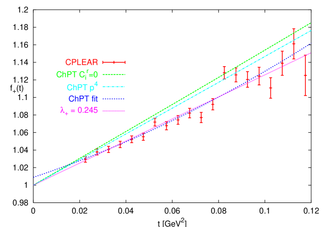
Refer to caption
Figure 1: ChPT fits to the CPLEAR data showing the effect of the curvature compared to fits without it.
$${R_{+1}^{K\pi}}=-(4.7\pm 0.5)~{}10^{-5}~{}\mbox{GeV}^{2}\quad\mbox{and}\quad\lambda_{+}=0.0170\pm 0.0015\,.$$ (8)

The first can be compared to the VMD estimate $\!{}^{{\bf?}}$ ${R_{+1}^{K\pi}|_{VMD}}\approx-4~{}10^{-5}~{}\mbox{GeV}^{2}$. The latter comes from ChPT as

$$\lambda_{+}=0.0283~{}(p^{4})~{}~{}+0.0011~{}(\mbox{loops }p^{6})~{}~{}-0.0124(C_{i}^{r})\,.$$ (9)

5 $f_{0}(t)$: theory

The $p^{6}$ result for $f_{0}(t)$ can be rewritten as

$\displaystyle f_{0}(t)$ $\displaystyle=$ $\displaystyle 1-\frac{8}{F_{\pi}^{4}}{\left(C_{12}^{r}+C_{34}^{r}\right)}\left(m_{K}^{2}-m_{\pi}^{2}\right)^{2}+8\frac{t}{F_{\pi}^{4}}{\left(2C_{12}^{r}+C_{34}^{r}\right)}\left(m_{K}^{2}+m_{\pi}^{2}\right)$ (10)
$\displaystyle+\frac{t}{m_{K}^{2}-m_{\pi}^{2}}\left(F_{K}/F_{\pi}-1\right)-\frac{8}{F_{\pi}^{4}}t^{2}{C_{12}^{r}}+\overline{\Delta}(t)+\Delta(0)\,.$

$\overline{\Delta}(t)$ and $\Delta(0)$ contain NO $C_{i}^{r}$ and only depend on the $L_{i}^{r}$ at order $p^{6}$ thus ALL needed parameters can be determined experimentally.

$$\Delta(0)=-0.0080\pm 0.0057[\mbox{loops}]\pm 0.0028[L_{i}^{r}]\,.$$ (11)

is known and an expression for $\Delta(t)$ can be found in Ref. $\!{}^{{\bf?}}$ The errors are an estimate of higher orders and using fits of the $L_{i}^{r}$ using different assumptions.

6 Conclusions

I have discussed the calculation of the $K_{\ell 3}$ form factors in ChPT at order $p^{6}$. The main conclusions are that the curvatures for $f_{+}(t)$ and $f_{0}(t)$ can be predicted from ChPT and the data on pion electromagnetic $\!{}^{{\bf?}}$ and scalar $\!{}^{{\bf?}}$ form-factors, the curvature in $f_{+}(t)$ and $f_{0}(t)$ should be taken into account in new precision experiments but from the slope and the curvature we can determine experimentally the needed parameters to calculate $f_{+}(0)$. A precision of better than one percent seems feasible for $|V_{us}|$.

Acknowledgments

This work has been funded in part by the Swedish Research Council and the European Union RTN network, Contract No. HPRN-CT-2002-00311 (EURIDICE)

References

References

  • [1] M. Battaglia et al., hep-ph/0304132.
  • [2] J. Bijnens and P. Talavera, hep-ph/0303103.
  • [3] J. Bijnens and P. Dhonte, work in progress.
  • [4] S. Weinberg, S. Weinberg, Physica A 96 (1979) 327;
    J. Gasser and H. Leutwyler, Annals Phys.  158 (1984) 142,
  • [5] J. Gasser and H. Leutwyler, Nucl. Phys. B 250 (1985) 465.
  • [6] A. Pich, A., hep-ph/9806303; G. Ecker, hep-ph/0011026; S. Scherer, hep-ph/0210398.
  • [7] J. Bijnens, G. Colangelo and G. Ecker, JHEP 9902 (1999) 020 [hep-ph/9902437];
  • [8] J. Bijnens, G. Colangelo and G. Ecker, Annals Phys.  280 (2000) 100 [hep-ph/9907333].
  • [9] G. Amorós, J. Bijnens and P. Talavera, Nucl. Phys. B 568 (2000) 319 [hep-ph/9907264], Nucl. Phys. B 602 (2001) 87 [hep-ph/0101127].
  • [10] G. Amorós, J. Bijnens and P. Talavera, Phys. Lett. B 480 (2000) 71 [hep-ph/9912398]; Nucl. Phys. B 585 (2000) 293 [Erratum-ibid. B 598 (2001) 665] [hep-ph/0003258].
  • [11] J. Bijnens and P. Talavera, JHEP 0203 (2002) 046 [hep-ph/0203049].
  • [12] H. Leutwyler and M. Roos, Z. Phys. C 25 (1984) 91.
  • [13] V. Cirigliano et al., Eur. Phys. J. C 23 (2002) 121 [hep-ph/0110153].
  • [14] A. Apostolakis et al. [CPLEAR Collaboration], Phys. Lett. B 473 (2000) 186.
  • [15] P. Post and K. Schilcher, Eur. Phys. J. C 25 (2002) 427 [hep-ph/0112352].