Vector Manifestation and Violation of Vector Dominance
in Hot Matter

Abstract

We show the details of the calculation of the hadronic thermal corrections to the two-point functions in the effective field theory of QCD for pions and vector mesons based on the hidden local symmetry (HLS) in hot matter using the background field gauge. We study the temperature dependence of the pion velocity in the low temperature region determined from the hadronic thermal corrections, and show that, due to the presence of the dynamical vector meson, the pion velocity is smaller than the speed of the light already at one-loop level, in contrast to the result obtained in the ordinary chiral perturbation theory including only the pion at one-loop. Including the intrinsic temperature dependences of the parameters of the HLS Lagrangian determined from the underlying QCD through the Wilsonian matching, we show how the vector manifestation (VM), in which the massless vector meson becomes the chiral partner of pion, is realized at the critical temperature. We present a new prediction of the VM on the direct photon-$\pi$-$\pi$ coupling which measures the validity of the vector dominance (VD) of the electromagnetic form factor of the pion: We find that the VD is largely violated at the critical temperature, which indicates that the assumption of the VD made in several analyses on the dilepton spectra in hot matter may need to be weakened for consistently including the effect of the dropping mass of the vector meson.

1 Introduction

Spontaneous chiral symmetry breaking is one of the most important features in low energy QCD. The phenomena of the light pseudoscalar mesons (the pion and its flavor partner), which are regarded as the approximate Nambu-Goldstone bosons associated with the symmetry breaking, are well described by the symmetry property in the low energy region. This chiral symmetry is expected to be restored in hot and/or dense matter and properties of hadrons will be changed near the critical point of the chiral symmetry restoration  HatsudaKunihiro ; Pisarski:95 ; Brown-Rho:96 ; Brown:2001nh ; HatsudaShiomiKuwabara ; Rapp-Wambach:00 ; Wilczek . It is important to investigate the physics near the phase transition point both theoretically and experimentally. In fact, the CERN Super Proton Synchrotron (SPS) observed an enhancement of dielectron ($e^{+}e^{-}$) mass spectra below the $\rho/\omega$ resonance Agakishiev:1995xb . This can be explained by the dropping mass of the $\rho$ meson (see, e.g., Refs. Li:1995qm ; Brown-Rho:96 ; Rapp-Wambach:00 ) following the Brown-Rho scaling proposed in Ref. BR . Furthermore, the Relativistic Heavy Ion Collider (RHIC) has started to measure several physical processes in hot matter which include the dilepton energy spectra. This will further clarify the properties of vector mesons in hot matter. Therefore it is interesting to study the properties of the pion and vector mesons near the critical temperature, especially associated with the dropping mass of the vector meson.

There is no strong restriction concerning vector meson masses in the standard scenario of chiral symmetry restoration, where the pion joins with the scalar meson in the same chiral representation [see for example, Refs. HatsudaKunihiro ; Bochkarev:1995gi ; PT:96 ]. However there is a scenario which certainly requires the dropping mass of the vector meson and supports the Brown-Rho scaling: In Ref. HYb , it was proposed that there can be another possibility for the pattern of chiral symmetry restoration, named the vector manifestation (VM). The VM was proposed as a novel manifestation of the chiral symmetry in the Wigner realization, in which the chiral symmetry is restored by the massless degenerate pion (and its flavor partners) and the longitudinal $\rho$ meson (and its flavor partners) as the chiral partner. In terms of the chiral representations of the low-lying mesons, there is a representation mixing in the vacuum HYb ; HYc . When we approach the critical point, there are two possibilities for the pattern of the chiral symmetry restoration: One possible pattern is the standard scenario and another is the VM. Both of them are on an equal footing with each other in terms of the chiral representations. It is worthwhile to study the physics associated with the VM as well as that with the standard scenario of the chiral symmetry restoration.

It has been shown that the VM is formulated at a large number of flavor HYb , critical temperature HSasaki and critical density HKR by using the effective field theory including both pions and vector mesons based on the hidden local symmetry (HLS) BKUYY ; BKYa , where a second order or weakly first order phase transition was assumed. In the VM at finite temperature and/or density, the intrinsic temperature and/or density dependences of the parameters of the HLS Lagrangian played important roles to realize the chiral symmetry restoration consistently: In the framework of the HLS the equality between the axial vector and vector current correlators at the critical point can be satisfied only if the intrinsic thermal and/or density effects are included. The intrinsic temperature and/or density dependences are nothing but the information converted from the underlying QCD through the Wilsonian matching HYa ; HSasaki . In Ref. HKRS , the predictions of the VM were made on the pion velocity and the vector and axial vector susceptibilities. It was stressed that the vector mesons in addition to the pseudoscalar mesons become relevant degrees of freedom near the critical temperature.

In this paper we shed some light on the validity of the vector dominance (VD) in hot matter. In several analyses such as the one on the dilepton spectra in hot matter carried out in Ref. Rapp-Wambach:00 , the VD is assumed to be held even in the high temperature region. There are several analyses resulting in the dropping mass consistent with the VD, as shown in Refs. GomezNicola:2002tn ; Dobado:2002xf . On the other hand, the analysis done in Ref. Pisarski shows that the thermal vector meson mass goes up if the VD holds. Thus, it is interesting to study what the VM predicts on the VD. In the present analysis we present a new prediction of the VM in hot matter on the direct photon-$\pi$-$\pi$ coupling which measures the validity of the VD of the electromagnetic form factor of the pion. We find that the VM predicts a large violation of the VD at the critical temperature. This indicates that the assumption of the VD may need to be weakened, at least in some amounts, for consistently including the effect of the dropping mass of the vector meson.

This paper is organized as follows: In section 2, we show the HLS Lagrangian which we use in the present analysis. In section 3, we present an entire list of the hadronic thermal corrections to the two-point functions including the vector and pseudoscalar meson loop contributions in the background field gauge. We think that it is useful to summarize the entire list of the hadronic thermal corrections since only the relevant part of them was listed in Ref. HKRS . In section 4, we first give an account of the general idea of the intrinsic thermal and/or dense effects, which was not explicitly stated before. Then, following Ref. HKRS , we briefly review how to extend the Wilsonian matching to the version at non-zero temperature to incorporate the intrinsic thermal effect. In section 5, we show the explicit forms of the pole masses of the longitudinal and transverse modes of the vector meson at non-zero temperature. Including the intrinsic thermal effect through the Wilsonian matching, we show how the VM is formulated at the critical temperature. In section 6, we study the temperature dependences of the temporal and spatial pion decay constants and the pion velocity in the low temperature region. The estimation of the value of the critical temperature is also carried out in wider range of input parameters than the one used in Ref. HSasaki . In section 7, we study the validity of the VD in hot matter, and show that the VD is largely violated near critical temperature. In section 8, we give a summary and discussions. Several functions and formulas used in this paper are listed in Appendices A-D.

2 Hidden Local Symmetry

In this section, we show the Lagrangian based on the hidden local symmetry (HLS) which we use in the present analysis.

The HLS model is based on the $G_{\rm{global}}\times H_{\rm{local}}$ symmetry, where $G=SU(N_{f})_{L}\times SU(N_{f})_{R}$ is the chiral symmetry and $H=SU(N_{f})_{V}$ is the HLS. The basic quantities are the HLS gauge boson and two matrix valued variables $\xi_{L}(x)$ and $\xi_{R}(x)$ which transform as

$$\xi_{L,R}(x)\to\xi^{\prime}_{L,R}(x)=h(x)\xi_{L,R}(x)g^{\dagger}_{L,R}\ ,$$ (1)

where $h(x)\in H_{\rm{local}}\ \mbox{and}\ g_{L,R}\in[\mbox{SU}(N_{f})_{\rm L,R}]_{\rm{global}}$. These variables are parameterized as

$$\xi_{L,R}(x)=e^{i\sigma(x)/{F_{\sigma}}}e^{\mp i\pi(x)/{F_{\pi}}}\ ,$$ (2)

where $\pi=\pi^{a}T_{a}$ denotes the pseudoscalar Nambu-Goldstone bosons associated with the spontaneous symmetry breaking of $G_{\rm{global}}$ chiral symmetry, and $\sigma=\sigma^{a}T_{a}$ denotes the Nambu-Goldstone bosons associated with the spontaneous breaking of $H_{\rm{local}}$. This $\sigma$ is absorbed into the HLS gauge boson through the Higgs mechanism. $F_{\pi}\ \mbox{and}\ F_{\sigma}$ are the decay constants of the associated particles. The phenomenologically important parameter $a$ is defined as

$$a=\frac{{F_{\sigma}}^{2}}{{F_{\pi}}^{2}}\ .$$ (3)

The covariant derivatives of $\xi_{L,R}$ are given by

$$D_{\mu}\xi_{L} = \partial_{\mu}\xi_{L}-iV_{\mu}\xi_{L}+i\xi_{L}{\cal{L}}_{\mu},$$

$$D_{\mu}\xi_{R} = \partial_{\mu}\xi_{R}-iV_{\mu}\xi_{R}+i\xi_{R}{\cal{R}}_{\mu},$$ (4)

where $V_{\mu}$ is the gauge field of $H_{\rm{local}}$, and ${\cal{L}}_{\mu}\ \mbox{and}\ {\cal{R}}_{\mu}$ are the external gauge fields introduced by gauging the $G_{\rm{global}}$ symmetry.

The HLS Lagrangian with the lowest derivative terms in the chiral limit is given by BKUYY ; BKYa

$${\cal{L}}_{(2)}={F_{\pi}}^{2}\mbox{tr}\bigl{[}\hat{\alpha}_{\perp\mu}\hat{\alpha}_{\perp}^{\mu}\bigr{]}+{F_{\sigma}}^{2}\mbox{tr}\bigl{[}\hat{\alpha}_{\parallel\mu}\hat{\alpha}_{\parallel}^{\mu}\bigr{]}-\frac{1}{2g^{2}}\mbox{tr}\bigl{[}V_{\mu\nu}V^{\mu\nu}\bigr{]}\ ,$$ (5)

where $g$ is the HLS gauge coupling, $V_{\mu\nu}$ is the field strength of $V_{\mu}$ and

$$\hat{\alpha}_{\perp}^{\mu} = \frac{1}{2i}\bigl{[}D^{\mu}\xi_{R}\cdot\xi_{R}^{\dagger}-D^{\mu}\xi_{L}\cdot\xi_{L}^{\dagger}\bigr{]}\ ,$$

$$\hat{\alpha}_{\parallel}^{\mu} = \frac{1}{2i}\bigl{[}D^{\mu}\xi_{R}\cdot\xi_{R}^{\dagger}+D^{\mu}\xi_{L}\cdot\xi_{L}^{\dagger}\bigr{]}\ .$$ (6)

In the HLS, as first pointed in Ref. Georgi and developed further in Refs. HYd ; Tana ; HYa ; HYc , thanks to the gauge symmetry, a systematic loop expansion can be formally performed with the vector mesons included in addition to the pseudoscalar mesons. In this chiral perturbation theory (ChPT) with HLS the vector meson mass is considered as small compared with the chiral symmetry breaking scale $\Lambda_{\chi}$, by assigning ${\cal O}(p)$ to the HLS gauge coupling Georgi ; Tana :

$$g\sim{\cal O}(p).$$ (7)

According to the entire list shown in Ref. Tana , there are 35 counter terms at ${\cal O}(p^{4})$ for general $N_{f}$. However, only three terms are relevant when we consider two-point functions in the chiral limit:

$${\cal{L}}_{(4)}=z_{1}\mbox{tr}\bigl{[}\hat{\cal{V}}_{\mu\nu}\hat{\cal{V}}^{\mu\nu}\bigr{]}+z_{2}\mbox{tr}\bigl{[}\hat{\cal{A}}_{\mu\nu}\hat{\cal{A}}^{\mu\nu}\bigr{]}+z_{3}\mbox{tr}\bigl{[}\hat{\cal{V}}_{\mu\nu}V^{\mu\nu}\bigr{]},$$ (8)

where

$$\hat{\cal{A}}_{\mu\nu}=\frac{1}{2}\bigl{[}\xi_{R}{\cal{R}}_{\mu\nu}\xi_{R}^{\dagger}-\xi_{L}{\cal{L}}_{\mu\nu}\xi_{L}^{\dagger}\bigr{]}\ ,$$ (9)

$$\hat{\cal{V}}_{\mu\nu}=\frac{1}{2}\bigl{[}\xi_{R}{\cal{R}}_{\mu\nu}\xi_{R}^{\dagger}+\xi_{L}{\cal{L}}_{\mu\nu}\xi_{L}^{\dagger}\bigr{]}\ ,$$ (10)

with ${\cal{R}}_{\mu\nu}\ \mbox{and}\ {\cal{L}}_{\mu\nu}$ being the field strengths of ${\cal{R}}_{\mu}\ \mbox{and}\ {\cal{L}}_{\mu}$.

In Ref. HYa , based on the ChPT with HLS, the Wilsonian matching was proposed, through which the parameters of the HLS Lagrangian are determined by the underlying QCD at the matching scale $\Lambda$. (For a review of the ChPT with HLS, the Wilsonian matching and VM at zero temperature, see Ref. HYc .) The Wilsonian matching at $T=0$ with $N_{f}=3$, where the validity of the ChPT with HLS is essential, was shown to give several predictions in remarkable agreement with experiments HYa ; HYc . This strongly suggests that the ChPT with HLS is valid even numerically. In Ref. HSasaki , we applied the ChPT with HLS combined with the Wilsonian matching to finite temperature. There the expansion parameter is $T/F_{\pi}(\Lambda)$ instead of $T/F_{\pi}(0)$ used in the standard ChPT. Since $F_{\pi}(\Lambda)>F_{\pi}(0)$, we think that the present formalism can be applied in the higher temperature region than the standard ChPT.

3 Two-Point Functions in Background Field Gauge

In the present approach hadronic thermal effects are included by calculating loop contributions of the pseudoscalar and vector meson. In Ref. HSasaki we used hadronic thermal corrections to the pion decay constant and vector meson mass calculated within the framework of the chiral perturbation theory with HLS in the Landau gauge. While in Ref. HKRS hadronic thermal corrections were calculated in the background field gauge. (For the application of the background field gauge to the HLS, see, e.g., Ref. HYc .) In this section we show details of the calculation of the hadronic thermal corrections to the two-point functions in the background field gauge.

Let us consider the loop corrections to the two-point functions at non-zero temperature. As was done in Ref. HKRS (see also section 4), we neglect the possible Lorentz symmetry violating effects caused by the intrinsic temperature dependences of the bare parameters in the present analysis. So we calculate loop corrections at non-zero temperature from the bare Lagrangian with Lorentz invariance shown in Eq. (5). For this purpose it is convenient to introduce the following functions:

$$A_{0}(M^{2};T) \equiv T\sum_{n=-\infty}^{\infty}\int\frac{d^{3}k}{(2\pi)^{3}}\frac{1}{M^{2}-k^{2}}\ ,$$ (11)

$$B_{0}(p_{0},\bar{p};M_{1},M_{2};T) \equiv T\sum_{n=-\infty}^{\infty}\int\frac{d^{3}k}{(2\pi)^{3}}\frac{1}{[M_{1}^{2}-k^{2}][M_{2}^{2}-(k-p)^{2}]}\ ,$$ (12)

$$B^{\mu\nu}(p_{0},\bar{p};M_{1},M_{2};T) \equiv T\sum_{n=-\infty}^{\infty}\int\frac{d^{3}k}{(2\pi)^{3}}\frac{\left(2k-p\right)^{\mu}\left(2k-p\right)^{\nu}}{[M_{1}^{2}-k^{2}][M_{2}^{2}-(k-p)^{2}]}\ ,$$ (13)

where $\bar{p}=|\vec{p}|$ and the $0$th component of the loop momentum is taken as $k^{0}=i2n\pi T$, while that of the external momentum is taken as $p^{0}=i2n^{\prime}\pi T$ [$n,n^{\prime}$: integer]. Using the standard formula (see, e.g., Ref. Kap ), these functions are divided into two parts as

$$A_{0}(M;T) = A_{0}^{\rm(vac)}(M)+\overline{A}_{0}(M;T)\ ,$$ (14)

$$B_{0}(p_{0},\bar{p};M_{1},M_{2};T) = B_{0}^{\rm(vac)}(p;M_{1},M_{2})+\overline{B}_{0}(p_{0},\bar{p};M_{1},M_{2};T)\ ,$$ (15)

$$B^{\mu\nu}(p_{0},\bar{p};M_{1},M_{2};T) = B^{{\rm(vac)}\mu\nu}(p;M_{1},M_{2})+\overline{B}^{\mu\nu}(p_{0},\bar{p};M_{1},M_{2};T)\ ,$$ (16)

where $A_{0}^{\rm(vac)}$, $B_{0}^{\rm(vac)}$ and $B^{{\rm(vac)}\mu\nu}$ express the quantum corrections given in Eqs. (C.30)–(C.32), and $\overline{A}_{0}$, $\overline{B}_{0}$ and $\overline{B}^{\mu\nu}$ the hadronic thermal corrections. We summarize the explicit forms of the functions $\overline{A}_{0}$, $\overline{B}_{0}$ and $\overline{B}^{\mu\nu}$ in various limits relevant to the present analysis in Appendix B. Note that the $0$th component of the momentum $p_{0}$ in the right-hand-sides of the above expressions is analytically continued to the Minkowski variable: $p_{0}$ is understood as $p_{0}+i\epsilon$ ($\epsilon\rightarrow+0$) for the retarded function and $p_{0}-i\epsilon$ for the advanced function. Then, $A_{0}^{\rm(vac)}$, $B_{0}^{\rm(vac)}$ and $B^{{\rm(vac)}\mu\nu}$ have no explicit temperature dependence, while they have intrinsic temperature dependence which is introduced through the Wilsonian matching as we will see later. In the following we write the two-point functions of $\overline{\cal A}_{\mu}$-$\overline{\cal A}_{\nu}$, $\overline{\cal V}_{\mu}$-$\overline{\cal V}_{\nu}$, $\overline{V}_{\mu}$-$\overline{V}_{\nu}$ and $\overline{V}_{\mu}$-$\overline{\cal V}_{\nu}$ as $\Pi_{\perp}^{\mu\nu}$, $\Pi_{\parallel}^{\mu\nu}$, $\Pi_{V}^{\mu\nu}$ and $\Pi_{V\parallel}^{\mu\nu}$, respectively.

At non-zero temperature there are four independent polarization tensors, which we choose as defined in Appendix A. We decompose the two-point functions $\Pi_{\perp}^{\mu\nu}$, $\Pi_{V}^{\mu\nu}$ $\Pi_{V\parallel}^{\mu\nu}$ and $\Pi_{\parallel}^{\mu\nu}$ as

$$\Pi_{\perp}^{\mu\nu} = u^{\mu}u^{\nu}\Pi_{\perp}^{t}+(g^{\mu\nu}-u^{\mu}u^{\nu})\Pi_{\perp}^{s}+P_{L}^{\mu\nu}\Pi_{\perp}^{L}+P_{T}^{\mu\nu}\Pi_{\perp}^{T}\ ,$$ (17)

$$\Pi_{V}^{\mu\nu} = u^{\mu}u^{\nu}\Pi_{V}^{t}+(g^{\mu\nu}-u^{\mu}u^{\nu})\Pi_{V}^{s}+P_{L}^{\mu\nu}\Pi_{V}^{L}+P_{T}^{\mu\nu}\Pi_{V}^{T}\ ,$$ (18)

$$\Pi_{V\parallel}^{\mu\nu} = u^{\mu}u^{\nu}\Pi_{V\parallel}^{t}+(g^{\mu\nu}-u^{\mu}u^{\nu})\Pi_{V\parallel}^{s}+P_{L}^{\mu\nu}\Pi_{V\parallel}^{L}+P_{T}^{\mu\nu}\Pi_{V\parallel}^{T}\ ,$$ (19)

$$\Pi_{\parallel}^{\mu\nu} = u^{\mu}u^{\nu}\Pi_{\parallel}^{t}+(g^{\mu\nu}-u^{\mu}u^{\nu})\Pi_{\parallel}^{s}+P_{L}^{\mu\nu}\Pi_{\parallel}^{L}+P_{T}^{\mu\nu}\Pi_{\parallel}^{T}\ ,$$ (20)

where $u^{\mu}=(1,\vec{0})$ and $P_{L}^{\mu\nu}$ and $P_{T}^{\mu\nu}$ are defined in Eq. (A.1). Similarly, we decompose the function $B^{\mu\nu}$ as

$$B^{\mu\nu}=u^{\mu}u^{\nu}B^{t}+(g^{\mu\nu}-u^{\mu}u^{\nu})B^{s}+P_{L}^{\mu\nu}B^{L}+P_{T}^{\mu\nu}B^{T}\ .$$ (21)

Furthermore, similarly to the division of the functions into one part for expressing the quantum correction and another for the hadronic thermal correction done in Eqs. (14)–(16), we divide the two-point functions into two parts as

$$\Pi^{\mu\nu}(p_{0},\bar{p};T)=\Pi^{\rm{(vac)}\mu\nu}(p_{0},\bar{p})+\overline{\Pi}^{\mu\nu}(p_{0},\bar{p};T)\ .$$ (22)

Accordingly each of four components of the two-point functions defined in Eqs. (17)–(20) is divided into the one part for the quantum correction and another for the hadronic thermal correction. We note that all the divergences are included in the zero temperature part $\Pi^{\rm(vac)}$.

Now, let us present the entire list of the hadronic thermal corrections to the two-point functions. (For the explicit forms of the quantum corrections $\Pi^{\rm(vac)}$, see Appendix C.)

We show the diagrams for contributions to $\Pi_{\perp}^{\mu\nu}$ at one-loop level in Fig. 1.

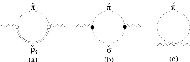
Figure 1: Diagrams for contributions to $\Pi_{\perp}^{\mu\nu}$ at one-loop level. The circle $(\circ)$ denotes the momentum-independent vertex and the dot $(\bullet)$ denotes the momentum-dependent vertex.

The temperature dependent parts are obtained as

$$\overline{\Pi}_{\perp}^{t}(p_{0},\bar{p};T) = -N_{f}aM_{\rho}^{2}\overline{B}_{0}(p_{0},\bar{p};M_{\rho},0;T)+N_{f}\frac{a}{4}\overline{B}^{t}(p_{0},\bar{p};M_{\rho},0;T)$$ (23)

$${}+N_{f}(a-1)\overline{A}_{0}(0;T),$$

$$\overline{\Pi}_{\perp}^{s}(p_{0},\bar{p};T) = -N_{f}aM_{\rho}^{2}\overline{B}_{0}(p_{0},\bar{p};M_{\rho},0;T)+N_{f}\frac{a}{4}\overline{B}^{s}(p_{0},\bar{p};M_{\rho},0;T)$$ (24)

$${}+N_{f}(a-1)\overline{A}_{0}(0;T),$$

$$\overline{\Pi}_{\perp}^{L}(p_{0},\bar{p};T) = N_{f}\frac{a}{4}\overline{B}^{L}(p_{0},\bar{p};M_{\rho},0;T),$$ (25)

$$\overline{\Pi}_{\perp}^{T}(p_{0},\bar{p};T) = N_{f}\frac{a}{4}\overline{B}^{T}(p_{0},\bar{p};M_{\rho},0;T).$$ (26)

As we will see later in section 5, we define the vector meson mass as the pole of longitudinal or transverse component of the vector meson propagator. The diagrams for contributions to $\Pi_{V}^{\mu\nu}$ are shown in Fig. 2.

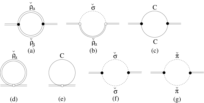
Figure 2: Diagrams for contributions to $\Pi_{V}^{\mu\nu}$ at one-loop level.

We obtain the hadronic thermal corrections to $\overline{\Pi}_{V}^{\mu\nu}$ as

$$\overline{\Pi}_{V}^{t}(p_{0},\bar{p};T) = 2N_{f}\overline{A}_{0}(M_{\rho};T)-M_{\rho}^{2}N_{f}\overline{B}_{0}(p_{0},\bar{p};M_{\rho},M_{\rho};T)$$ (27)

$${}+\frac{a^{2}}{8}N_{f}\overline{B}^{t}(p_{0},\bar{p};0,0;T){}+\frac{9}{8}N_{f}\overline{B}^{t}(p_{0},\bar{p};M_{\rho},M_{\rho};T)\ ,$$

$$\overline{\Pi}_{V}^{s}(p_{0},\bar{p};T) = 2N_{f}\overline{A}_{0}(M_{\rho};T)-M_{\rho}^{2}N_{f}\overline{B}_{0}(p_{0},\bar{p};M_{\rho},M_{\rho};T)$$ (28)

$${}+\frac{a^{2}}{8}N_{f}\overline{B}^{s}(p_{0},\bar{p};0,0;T){}+\frac{9}{8}N_{f}\overline{B}^{s}(p_{0},\bar{p};M_{\rho},M_{\rho};T)\ ,$$

$$\overline{\Pi}_{V}^{L}(p_{0},\bar{p};T) = -4p^{2}N_{f}\overline{B}_{0}(p_{0},\bar{p};M_{\rho},M_{\rho};T)$$ (29)

$${}+\frac{a^{2}}{8}N_{f}\overline{B}^{L}(p_{0},\bar{p};0,0;T){}+\frac{9}{8}N_{f}\overline{B}^{L}(p_{0},\bar{p};M_{\rho},M_{\rho};T),$$

$$\overline{\Pi}_{V}^{T}(p_{0},\bar{p};T) = -4p^{2}N_{f}\overline{B}_{0}(p_{0},\bar{p};M_{\rho},M_{\rho};T)$$ (30)

$${}+\frac{a^{2}}{8}N_{f}\overline{B}^{T}(p_{0},\bar{p};0,0;T){}+\frac{9}{8}N_{f}\overline{B}^{T}(p_{0},\bar{p};M_{\rho},M_{\rho};T).$$

Another two-point function associated with the vector current correlator is $\Pi_{V\parallel}^{\mu\nu}$. We also show the one-loop diagrams for contributions to $\Pi_{V\parallel}^{\mu\nu}$ in Fig. 3.

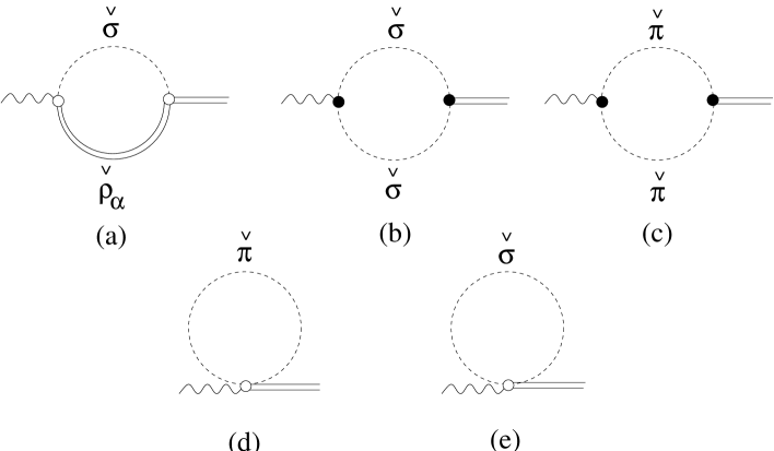
Figure 3: Diagrams for contributions to $\Pi_{V\parallel}^{\mu\nu}$ at one-loop level.

We get the temperature dependent parts as

$$\overline{\Pi}_{V\parallel}^{t}(p_{0},\bar{p};T) = \frac{a}{2}N_{f}\overline{A}_{0}(0;T){}+\frac{1}{2}N_{f}\overline{A}_{0}(M_{\rho};T){}+N_{f}M_{\rho}^{2}\overline{B}_{0}(p_{0},\bar{p};M_{\rho},M_{\rho};T)$$ (31)

$${}+\frac{1}{8}N_{f}\overline{B}^{t}(p_{0},\bar{p};M_{\rho},M_{\rho};T){}+\frac{a(2-a)}{8}N_{f}\overline{B}^{t}(p_{0},\bar{p};0,0;T),$$

$$\overline{\Pi}_{V\parallel}^{s}(p_{0},\bar{p};T) = \frac{a}{2}N_{f}\overline{A}_{0}(0;T){}+\frac{1}{2}N_{f}\overline{A}_{0}(M_{\rho};T){}+N_{f}M_{\rho}^{2}\overline{B}_{0}(p_{0},\bar{p};M_{\rho},M_{\rho};T)$$ (32)

$${}+\frac{1}{8}N_{f}\overline{B}^{s}(p_{0},\bar{p};M_{\rho},M_{\rho};T){}+\frac{a(2-a)}{8}N_{f}\overline{B}^{s}(p_{0},\bar{p};0,0;T),$$

$$\overline{\Pi}_{V\parallel}^{L}(p_{0},\bar{p};T) = \frac{1}{8}N_{f}\overline{B}^{L}(p_{0},\bar{p};M_{\rho},M_{\rho};T){}+\frac{a(2-a)}{8}N_{f}\overline{B}^{L}(p_{0},\bar{p};0,0;T),$$ (33)

$$\overline{\Pi}_{V\parallel}^{T}(p_{0},\bar{p};T) = \frac{1}{8}N_{f}\overline{B}^{T}(p_{0},\bar{p};M_{\rho},M_{\rho};T){}+\frac{a(2-a)}{8}N_{f}\overline{B}^{T}(p_{0},\bar{p};0,0;T).$$ (34)

In section 7, we will define the parameter $a$ from the direct $\gamma\pi\pi$ coupling using the two-point function $\Pi_{\parallel}^{\mu\nu}$. We show the diagrams for contributions to $\Pi_{\parallel}^{\mu\nu}$ at one-loop level in Fig. 4.

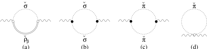
Figure 4: Diagrams for contributions to $\Pi_{\parallel}^{\mu\nu}$ at one-loop level.

We get the temperature dependent parts as

$$\overline{\Pi}_{\parallel}^{t}(p_{0},\bar{p};T) = -(a-1)N_{f}\overline{A}_{0}(0;T){}-N_{f}M_{\rho}^{2}\overline{B}_{0}(p_{0},\bar{p};M_{\rho},M_{\rho};T)$$ (35)

$${}+\frac{1}{8}N_{f}\overline{B}^{t}(p_{0},\bar{p};M_{\rho},M_{\rho};T){}+\frac{(2-a)^{2}}{8}N_{f}\overline{B}^{t}(p_{0},\bar{p};0,0;T)\ ,$$

$$\overline{\Pi}_{\parallel}^{s}(p_{0},\bar{p};T) = -(a-1)N_{f}\overline{A}_{0}(0;T){}-N_{f}M_{\rho}^{2}\overline{B}_{0}(p_{0},\bar{p};M_{\rho},M_{\rho};T)$$ (36)

$${}+\frac{1}{8}N_{f}\overline{B}^{s}(p_{0},\bar{p};M_{\rho},M_{\rho};T){}+\frac{(2-a)^{2}}{8}N_{f}\overline{B}^{s}(p_{0},\bar{p};0,0;T)\ ,$$

$$\overline{\Pi}_{\parallel}^{L}(p_{0},\bar{p};T) = \frac{1}{8}N_{f}\overline{B}^{L}(p_{0},\bar{p};M_{\rho},M_{\rho};T){}+\frac{(2-a)^{2}}{8}N_{f}\overline{B}^{L}(p_{0},\bar{p};0,0;T),$$ (37)

$$\overline{\Pi}_{\parallel}^{T}(p_{0},\bar{p};T) = \frac{1}{8}N_{f}\overline{B}^{T}(p_{0},\bar{p};M_{\rho},M_{\rho};T){}+\frac{(2-a)^{2}}{8}N_{f}\overline{B}^{T}(p_{0},\bar{p};0,0;T).$$ (38)

At the end of this section, using the relations shown in Eq. (B.18), we obtain

$$\overline{\Pi}_{V}^{t}=-\overline{\Pi}_{V\parallel}^{t}=\overline{\Pi}_{\parallel}^{t}$$

$$\quad=\overline{\Pi}_{V}^{s}=-\overline{\Pi}_{V\parallel}^{s}=\overline{\Pi}_{\parallel}^{s}$$

$$\quad=-N_{f}\frac{1}{4}\left[\overline{A}_{0}(M_{\rho};T)+\overline{A}_{0}(0;T)\right]-N_{f}M_{\rho}^{2}\overline{B}_{0}(p_{0},\bar{p};M_{\rho},M_{\rho};T)\ .$$ (39)

Since the quantum corrections to the corresponding components are identical as we have shown in Eq. (C.43), the above relation implies that the components $\Pi_{V}^{t}$, $\Pi_{V\parallel}^{t}$, $\Pi_{\parallel}^{t}$, $\Pi_{V}^{s}$, $\Pi_{V\parallel}^{s}$ and $\Pi_{\parallel}^{t}$ agree:

$$\Pi_{V}^{t}=-\Pi_{V\parallel}^{t}=\Pi_{\parallel}^{t}=\Pi_{V}^{s}=-\Pi_{V\parallel}^{s}=\Pi_{\parallel}^{s}\ .$$ (40)

This relation is important to prove the conservation of the vector current correlator as shown in Ref. HKRS . 

4 Intrinsic Thermal Effects

In this section, we first give an account of the general idea of the intrinsic temperature and/or density dependences of the bare parameters. Next, following Ref. HKRS , we briefly review how to extend the Wilsonian matching to the version at non-zero temperature in order to incorporate the intrinsic thermal effect into the bare parameters of the HLS Lagrangian. There we discuss the effect of Lorentz symmetry violation at bare level, and summarize the conditions for the bare parameters obtained in Ref. HSasaki through the Wilsonian matching at the critical temperature.

4.1 General Concept of the Intrinsic Thermal and/or Density Effects

In this subsection, we give a general idea of the matching between the effective field theory (EFT) and QCD. Green’s functions have important information of system, which is generated by the following functional of a set of source fields denoted by $J$:

$$Z[J]=\int{\cal D}q{\cal D}\bar{q}{\cal D}Ge^{S_{\rm QCD}[J]},$$ (41)

where $q$ $(\bar{q})$ denotes quark or antiquark field, $G$ is gluon field and $S_{\rm QCD}$ represents the action expressed in terms of the quarks and gluons. The basic concept of the EFT is that the effective Lagrangian, which has the most general form constructed from the chiral symmetry, can give the same generating functional as in Eq. (41):

$$Z[J]=\int{\cal D}Ue^{S_{\rm eff}[J]},$$ (42)

where $U$ denotes the relevant hadronic fields such as the pion fields and $S_{\rm eff}$ is the action expressed in terms of these hadrons. Corresponding to each Green’s function derived from Eq. (41), we have the same Green’s function obtained from the EFT through Eq. (42). Performing the matching between these two Green’s functions, we can determine the parameters of the EFT.

In some matching schemes, the renormalized parameters of the EFT are determined from QCD. On the other hand, the matching in the Wilsonian sense is performed based on the following general idea: The bare Lagrangian of the EFT is defined at a suitable matching scale $\Lambda$ and the generating functional derived from the bare Lagrangian leads to the same Green’s function as that derived from Eq. (41) at $\Lambda$. Then the bare parameters of the EFT are determined through the Wilsonian matching. In other words, we obtain the bare Lagrangian of the EFT after integrating out the high energy modes, i.e., the quarks and gluons above $\Lambda$. The information of the high energy modes is included in the parameters of the EFT. Thus when we integrate out high energy modes in hot and/or dense matter, the parameters are in general dependent on temperature and/or density. The intrinsic temperature and/or density dependences are nothing but the signature that the hadron has an internal structure constructed from the quarks and gluons. This is similar to the situation where the coupling constants among hadrons are replaced with the momentum-dependent form factor in the high energy region. Thus the intrinsic thermal and/or dense effects play more important roles in the higher temperature region, especially near the critical temperature.

4.2 Wilsonian Matching

The Wilsonian matching proposed in Ref. HYa is done by matching the axial vector and vector current correlators derived from the HLS with those from the operator product expansion (OPE) in QCD at the matching scale $\Lambda$ .

Here it should be noticed that there is no longer Lorentz symmetry in hot matter, and the Lorentz non-scalar operators such as $\bar{q}\gamma_{\mu}D_{\nu}q$ may exist in the form of the current correlators derived from the OPE HKL . This leads to a difference between the temporal and spatial bare pion decay constants. However, we neglect the contributions from these operators since they give a small correction compared with the main term $1+\frac{\alpha_{s}}{\pi}$ HSasaki . This implies that the Lorentz symmetry breaking effect in the bare pion decay constant is small, $F_{\pi,\rm{bare}}^{t}\simeq F_{\pi,\rm{bare}}^{s}$ HKRS . Thus to a good approximation we determine the pion decay constant at non-zero temperature through the matching condition at zero temperature, putting possible temperature dependences into the gluonic and quark condensates HSasaki ; HKRS :

$$\frac{F^{2}_{\pi}(\Lambda;T)}{{\Lambda}^{2}}=\frac{1}{8{\pi}^{2}}\Bigl{[}1+\frac{\alpha_{s}}{\pi}+\frac{2{\pi}^{2}}{3}\frac{\langle\frac{\alpha_{s}}{\pi}G_{\mu\nu}G^{\mu\nu}\rangle_{T}}{{\Lambda}^{4}}+{\pi}^{3}\frac{1408}{27}\frac{\alpha_{s}{\langle\bar{q}q\rangle}^{2}_{T}}{{\Lambda}^{6}}\Bigr{]}\ .$$ (43)

Through this condition the temperature dependences of the quark and gluonic condensates determine the intrinsic temperature dependences of the bare parameter $F_{\pi}(\Lambda;T)$, which is then converted into those of the on-shell parameter $F_{\pi}(\mu=0;T)$ through the Wilsonian RGEs.

Now, let us consider the Wilsonian matching near the chiral symmetry restoration point. Here we assume that the order of the chiral phase transition is second or weakly first order, and thus the quark condensate becomes zero continuously for $T\to T_{c}$. First, note that the Wilsonian matching condition (43) provides

$$\frac{F^{2}_{\pi}(\Lambda;T_{c})}{{\Lambda}^{2}}=\frac{1}{8{\pi}^{2}}\Bigl{[}1+\frac{\alpha_{s}}{\pi}+\frac{2{\pi}^{2}}{3}\frac{\langle\frac{\alpha_{s}}{\pi}G_{\mu\nu}G^{\mu\nu}\rangle_{T_{c}}}{{\Lambda}^{4}}\Bigr{]}\neq 0\ ,$$ (44)

which implies that the matching with QCD dictates

$$F^{2}_{\pi}(\Lambda;T_{c})\neq 0$$ (45)

even at the critical temperature where the on-shell pion decay constant vanishes by adding the quantum corrections through the RGE including the quadratic divergence HYa and hadronic thermal corrections, as we will show in section 6. As was shown in Ref. HKR for the VM in dense matter, the Lorentz non-invariant version of the VM conditions for the bare parameters are obtained by the requirement of the equality between the axial vector and vector current correlators in the HLS, which should be valid also in hot matter HKRS :

$$a_{\rm{bare}}^{t}\equiv\Biggl{(}\frac{F_{\sigma,\rm{bare}}^{t}}{F_{\pi,\rm{bare}}^{t}}\Biggr{)}^{2}\stackrel{{\scriptstyle T\to T_{c}}}{{\to}}1,\quad a_{\rm{bare}}^{s}\equiv\Biggl{(}\frac{F_{\sigma,\rm{bare}}^{s}}{F_{\pi,\rm{bare}}^{s}}\Biggr{)}^{2}\stackrel{{\scriptstyle T\to T_{c}}}{{\to}}1,$$ (46)

$$g_{T,\rm{bare}}\stackrel{{\scriptstyle T\to T_{c}}}{{\to}}0,\quad g_{L,\rm{bare}}\stackrel{{\scriptstyle T\to T_{c}}}{{\to}}0,$$ (47)

where $a^{t}_{\rm{bare}},a^{s}_{\rm{bare}},g_{T,\rm{bare}}$ and $g_{L,\rm{bare}}$ are the extensions of the parameters $a_{\rm{bare}}$ and $g_{\rm{bare}}$ in the bare Lagrangian with the Lorentz symmetry breaking effect included as in Appendix A of Ref. HKR .

When we use the conditions for the parameters $a^{t,s}$ in Eq. (46) and the above result that the Lorentz symmetry violation between the bare pion decay constants $F_{\pi,\rm{bare}}^{t,s}$ is small, we can easily show that the Lorentz symmetry breaking effect between the temporal and spatial bare sigma decay constants is also small, $F_{\sigma,\rm{bare}}^{t}\simeq F_{\sigma,\rm{bare}}^{s}$ HKRS . While we cannot determine the ratio $g_{L,\rm{bare}}/g_{T,\rm{bare}}$ through the Wilsonian matching since the transverse mode of vector meson decouples near the critical temperature.  However this implies that the transverse mode is irrelevant for the quantities studied in this paper. Therefore in the present analysis, we set $g_{L,\rm{bare}}=g_{T,\rm{bare}}$ for simplicity and use the Lorentz invariant Lagrangian at bare level. In the low temperature region, the intrinsic temperature dependences are negligible, so that we also use the Lorentz invariant Lagrangian at bare level as in the analysis by the ordinary chiral Lagrangian in Ref. GL .

At the critical temperature, the axial vector and vector current correlators derived in the OPE agree with each other for any value of $Q^{2}$. Thus we require that these current correlators in the HLS are equal at the critical temperature for any value of $Q^{2}\ \mbox{around}\ {\Lambda}^{2}$. As we discussed above, we start from the Lorentz invariant bare Lagrangian even in hot matter, and then the axial vector current correlator $G_{A}^{\rm{(HLS)}}$ and the vector current correlator $G_{V}^{\rm{(HLS)}}$ are expressed by the same forms as those at zero temperature with the bare parameters having the intrinsic temperature dependences:

$$G^{\rm{(HLS)}}_{A}(Q^{2};T) = \frac{F^{2}_{\pi}(\Lambda;T)}{Q^{2}}-2z_{2}(\Lambda;T),$$

$$G^{\rm{(HLS)}}_{V}(Q^{2};T) = \frac{F^{2}_{\sigma}(\Lambda;T)[1-2g^{2}(\Lambda;T)z_{3}(\Lambda;T)]}{{M_{\rho}}^{2}(\Lambda;T)+Q^{2}}-2z_{1}(\Lambda;T).$$ (48)

By taking account of the fact $F^{2}_{\pi}(\Lambda;T_{c})\neq 0$ derived from the Wilsonian matching condition given in Eq. (44), the requirement $G_{A}^{(\rm{HLS})}=G_{V}^{(\rm{HLS})}$ is satisfied only if the following conditions are met HSasaki :

$$g(\Lambda;T) \stackrel{{\scriptstyle T\to T_{c}}}{{\to}} 0,$$ (49)

$$a(\Lambda;T)=F_{\sigma}^{2}(\Lambda;T)/F_{\pi}^{2}(\Lambda;T) \stackrel{{\scriptstyle T\to T_{c}}}{{\to}} 1,$$ (50)

$$z_{1}(\Lambda;T)-z_{2}(\Lambda;T) \stackrel{{\scriptstyle T\to T_{c}}}{{\to}} 0.$$ (51)

Note that the intrinsic thermal effects act on the parameters in such a way that they become the values of Eqs. (49)-(51).

Through the Wilsonian matching at non-zero temperature mentioned above, the parameters appearing in the hadronic thermal corrections calculated in section 3 have the intrinsic temperature dependences: $F_{\pi}$, $a$ and $g$ appearing there should be regarded as

$$F_{\pi} \equiv F_{\pi}(\mu=0;T)\ ,$$

$$a \equiv a\left(\mu=M_{\rho}(T);T\right)\ ,$$

$$g \equiv g\left(\mu=M_{\rho}(T);T\right)\ ,$$ (52)

where $M_{\rho}$ is determined from the on-shell condition:

$$M_{\rho}^{2}\equiv M_{\rho}^{2}(T)=a(\mu=M_{\rho};T)g^{2}(\mu=M_{\rho};T)F_{\pi}^{2}(\mu=M_{\rho};T)\ .$$ (53)

From the RGEs for $g\ \mbox{and}\ a$ in Eqs.(C.58) and (C.57), we find that $(g,a)=(0,1)$ is the fixed point. Therefore, Eqs. (49) and (50) imply that $g$ and $a$ at the on-shell of the vector meson take the same values:

$$a\,(\mu=M_{\rho}(T);T)\ \mathop{\longrightarrow}^{T\rightarrow T_{c}}\ 1\ ,$$

$$g\,(\mu=M_{\rho}(T);T)\ \mathop{\longrightarrow}^{T\rightarrow T_{c}}\ 0\ ,$$ (54)

where the parametric vector meson mass $M_{\rho}(T)$ is determined from the condition (53). The above conditions with Eq. (53) imply that $M_{\rho}(T)$ also vanishes:

$$M_{\rho}(T)\ \mathop{\longrightarrow}^{T\rightarrow T_{c}}\ 0\ .$$ (55)

5 Vector Meson Mass

In Ref. HSasaki we have shown that the vector manifestation (VM) in hot matter can actually be formulated by using the hadronic thermal correction to the vector meson pole mass calculated in the Landau gauge HS . In Ref. HKRS the background field gauge was used to calculate the hadronic thermal corrections. There the vector meson pole mass was not explicitly studied. In this section we first define the vector meson pole masses of both the longitudinal and transverse modes at non-zero temperature from the vector current correlator in the background field gauge and show the explicit forms of the hadronic thermal corrections from the vector and pseudoscalar meson loop. Then, including the intrinsic temperature dependences of the parameters near the critical temperature determined in the previous section, we show that the vector meson mass vanishes at the critical temperature.

Let us define pole masses of longitudinal and transverse modes of the vector meson from the poles of longitudinal and transverse components of the vector current correlator in the rest frame HKRS :

$$G_{V}^{\mu\nu}=P_{L}^{\mu\nu}G_{V}^{L}+P_{T}^{\mu\nu}G_{V}^{T},$$ (56)

where

$$G_{V}^{L} = \frac{\Pi_{V}^{s}\bigl{(}\Pi_{V}^{L}+2\Pi_{V\parallel}^{L}\bigr{)}}{\Pi_{V}^{s}-\Pi_{V}^{L}}+\Pi_{\parallel}^{L},$$

$$G_{V}^{T} = \frac{\Pi_{V}^{s}\bigl{(}\Pi_{V}^{T}+2\Pi_{V\parallel}^{T}\bigr{)}}{\Pi_{V}^{s}-\Pi_{V}^{T}}+\Pi_{\parallel}^{T}.$$ (57)

Then, the pole masses are obtained as the solutions of the following on-shell conditions:

$$0=\mbox{Re}\left[\Pi_{V}^{s}(p_{0}=m_{\rho}^{L}(T),0;T)-\Pi_{V}^{L}(p_{0}=m_{\rho}^{L}(T),0;T)\right]\ ,$$

$$0=\mbox{Re}\left[\Pi_{V}^{s}(p_{0}=m_{\rho}^{T}(T),0;T)-\Pi_{V}^{T}(p_{0}=m_{\rho}^{T}(T),0;T)\right]\ ,$$ (58)

where $m_{\rho}^{L}(T)$ and $m_{\rho}^{T}(T)$ denote the pole masses of the longitudinal and transverse modes, respectively. As we have calculated in section 3, $\Pi_{V}^{s}(p_{0},\bar{p};T)$, $\Pi_{V}^{L}(p_{0},\bar{p};T)$ and $\Pi_{V}^{T}(p_{0},\bar{p};T)$ in the HLS at one-loop level are expressed as

$$\Pi_{V}^{s}(p_{0},\bar{p};T) = F_{\sigma}^{2}(M_{\rho})+\widetilde{\Pi}_{V}^{S}(p^{2})+\overline{\Pi}_{V}^{s}(p_{0},\bar{p};T)\ ,$$

$$\Pi_{V}^{L}(p_{0},\bar{p};T) = \frac{p^{2}}{g^{2}(M_{\rho})}+\widetilde{\Pi}_{V}^{LT}(p^{2})+\overline{\Pi}_{V}^{L}(p_{0},\bar{p};T)\ ,$$

$$\Pi_{V}^{T}(p_{0},\bar{p};T) = \frac{p^{2}}{g^{2}(M_{\rho})}+\widetilde{\Pi}_{V}^{LT}(p^{2})+\overline{\Pi}_{V}^{T}(p_{0},\bar{p};T)\ ,$$ (59)

where the explicit forms of the finite renormalization effects $\widetilde{\Pi}_{V}^{S}(p^{2})$ and $\widetilde{\Pi}_{V}^{LT}(p^{2})$ are given in Eqs. (C.60) and (C.61), and those of the hadronic thermal effects $\overline{\Pi}_{V}^{s}(p_{0},\bar{p};T)$, $\overline{\Pi}_{V}^{L}(p_{0},\bar{p};T)$ and $\overline{\Pi}_{V}^{T}(p_{0},\bar{p};T)$ are given in Eqs. (39), (29) and (30). Substituting Eq. (59) into Eq. (58), we obtain

$$\left[m_{\rho}^{L}(T)\right]^{2} = M_{\rho}^{2}{}+g^{2}(M_{\rho})\,\Biggl{[}\mbox{Re}\,\widetilde{\Pi}_{V}^{S}(p_{0}^{2})+\mbox{Re}\,\overline{\Pi}_{V}^{s}(p_{0},0;T)$$

$$\qquad\qquad\qquad{}-\mbox{Re}\,\widetilde{\Pi}_{V}^{T}(p_{0}^{2})-\mbox{Re}\,\overline{\Pi}_{V}^{L}(p_{0},0;T)\Biggr{]}_{p_{0}=m_{\rho}^{L}(T)}\ ,$$

$$\left[m_{\rho}^{T}(T)\right]^{2} = M_{\rho}^{2}{}+g^{2}(M_{\rho})\,\Biggl{[}\mbox{Re}\,\widetilde{\Pi}_{V}^{S}(p_{0}^{2})+\mbox{Re}\,\overline{\Pi}_{V}^{s}(p_{0},0;T)$$ (60)

$$\qquad\qquad\qquad{}-\mbox{Re}\,\widetilde{\Pi}_{V}^{T}(p_{0}^{2})-\mbox{Re}\,\overline{\Pi}_{V}^{T}(p_{0},0;T)\Biggr{]}_{p_{0}=m_{\rho}^{T}(T)}\ .$$

We can replace $m_{\rho}^{L}(T)$ and $m_{\rho}^{T}(T)$ with $M_{\rho}$ in the hadronic thermal effects as well as in the finite renormalization effect, since the difference is of higher order. Then, noting that $\mbox{Re}\,\widetilde{\Pi}_{V}^{S}(p^{2}=M_{\rho}^{2})=\mbox{Re}\,\widetilde{\Pi}_{V}^{LT}(p^{2}=M_{\rho}^{2})=0$ as shown in Eq. (C.48), we obtain

$$\left[m_{\rho}^{L}(T)\right]^{2} = M_{\rho}^{2}-g^{2}(M_{\rho})\,\mbox{Re}\left[\overline{\Pi}_{V}^{L}(M_{\rho};0;T)-\overline{\Pi}_{V}^{s}(M_{\rho};0;T)\right]\ ,$$ (61)

$$\left[m_{\rho}^{T}(T)\right]^{2} = M_{\rho}^{2}-g^{2}(M_{\rho})\,\mbox{Re}\left[\overline{\Pi}_{V}^{T}(M_{\rho};0;T)-\overline{\Pi}_{V}^{s}(M_{\rho};0;T)\right]\ .$$ (62)

Let us compute the explicit form of the pole mass using the expression of $\overline{\Pi}_{V}^{s}$, $\overline{\Pi}_{V}^{L}$ and $\overline{\Pi}_{V}^{T}$ calculated in section 3. Here we note that Eqs. (B.28) and (B.29) imply that $\overline{B}^{L}-\overline{B}^{s}$ agrees with $\overline{B}^{T}-\overline{B}^{s}$ in the rest frame. Then in the rest frame $\overline{\Pi}_{V}^{L}-\overline{\Pi}_{V}^{s}$ agrees with $\overline{\Pi}_{V}^{T}-\overline{\Pi}_{V}^{s}$. Thus the longitudinal pole mass is the same as the transverse one:

$$m_{\rho}^{L}(T)=m_{\rho}^{T}(T)\equiv m_{\rho}(T)\ .$$ (63)

By using the low momentum limits of the functions shown in Eqs. (B.27) and (B.28), $\overline{\Pi}^{L}_{V}-\overline{\Pi}^{s}_{V}$ in the rest frame is expressed as

$$\overline{\Pi}^{L}_{V}(p_{0},\bar{p}=0;T)-\overline{\Pi}^{s}_{V}(p_{0},\bar{p}=0;T)$$ (64)

$$= N_{f}\Bigl{[}\frac{a^{2}}{24}\tilde{G}_{2}(p_{0};T)-\tilde{J}_{1}^{2}(M_{\rho};T)+\bigl{(}\frac{M_{\rho}^{2}}{4}-p_{0}^{2}\bigr{)}\tilde{F}_{3}^{2}(p_{0};M_{\rho};T)+\frac{3}{8}\tilde{F}_{3}^{4}(p_{0};M_{\rho};T)\Bigr{]},$$

where the functions $\tilde{I}_{n}$, $\tilde{J}^{n}_{m}$, $\tilde{F}^{n}_{m}$ and $\tilde{G}^{n}_{m}$ are defined in Appendix D. Substituting the above expression into Eq. (61) and using the relation

$$-\frac{1}{3M_{\rho}^{2}}\tilde{F}_{3}^{4}(M_{\rho};M_{\rho};T) = \frac{1}{4}\tilde{F}_{3}^{2}(M_{\rho};M_{\rho};T)-\frac{1}{3M_{\rho}^{2}}\tilde{J}_{1}^{2}(M_{\rho};T)\ ,$$ (65)

we find that the vector meson pole mass is expressed as

$$m^{2}_{\rho}(T) = {M_{\rho}}^{2}+N_{f}\,g^{2}\Biggl{[}-\frac{a^{2}}{12}\tilde{G}_{2}(M_{\rho};T)+\frac{4}{5}\tilde{J}^{2}_{1}(M_{\rho};T)+\frac{33}{16}M_{\rho}^{2}\tilde{F}^{2}_{3}(M_{\rho};M_{\rho};T)\Biggr{]}.$$ (66)

The contribution in this expression agrees with the result in Ref. HSasaki which is derived from the hadronic thermal correction calculated in the Landau gauge in Ref. HS by taking the on-shell condition (61). 

Before going to the analysis near the critical temperature, we study the behavior of the pole mass in the low temperature region, $T\ll M_{\rho}$. In this region the functions $F^{n}_{m}$ and $J^{n}_{m}$ are suppressed by $e^{-M_{\rho}/T}$, and thus give negligible contributions. Since $G_{2}\approx-\frac{{\pi}^{4}}{15}\frac{T^{4}}{{M_{\rho}}^{2}}$, the vector meson pole mass increases as $T^{4}$ in the low temperature region, dominated by the $\pi$-loop effects:

$${m_{\rho}}^{2}(T)\approx{M_{\rho}}^{2}+\frac{N_{f}{\pi}^{2}a}{360{F_{\pi}}^{2}}T^{4}\qquad\mbox{for}\quad T\ll M_{\rho}.$$ (67)

Note that the lack of $T^{2}$-term in the above expression is consistent with the result by the current algebra analysis Dey-Eletsky-Ioffe .

Now, let us study the vector meson pole mass near the critical temperature. As shown in section 4, the intrinsic temperature dependences of the parameters of the HLS Lagrangian determined through the Wilsonian matching imply that the parametric vector meson mass $M_{\rho}$ vanishes at the critical temperature. Then, near the critical temperature we should take $M_{\rho}\ll T$ in Eq. (66) instead of $T\ll M_{\rho}$ which was taken to reach the expression in Eq. (67) in the low temperature region. Thus, by noting that

$$\tilde{G}_{2}(M_{\rho};T) \stackrel{{\scriptstyle M_{\rho}\to 0}}{{\to}} \tilde{I}_{2}(T),$$

$$\tilde{J}^{2}_{1}(M_{\rho};T) \stackrel{{\scriptstyle M_{\rho}\to 0}}{{\to}} \tilde{I}_{2}(T),$$

$${M_{\rho}}^{2}\tilde{F}^{2}_{3}(M_{\rho};M_{\rho};T) \stackrel{{\scriptstyle M_{\rho}\to 0}}{{\to}} 0,$$ (68)

the pole mass of the vector meson at $T\lesssim T_{c}$ becomes

$${m_{\rho}}^{2}(T) = {M_{\rho}}^{2}+N_{f}\,g^{2}\frac{15-a^{2}}{12}\tilde{I}_{2}(T)$$ (69)

$$= {M_{\rho}}^{2}+N_{f}\,g^{2}\frac{15-a^{2}}{144}T^{2}.$$

In the vicinity of $a\simeq 1$ the hadronic thermal effect gives a positive correction, and then the vector meson pole mass is actually larger than the parametric mass $M_{\rho}$. However, the intrinsic temperature dependences of the parameters obtained in section 4 lead to $g\to 0$ and $M_{\rho}\rightarrow 0$ for $T\to T_{c}$. Then, from Eq. (69) we conclude that the pole mass of the vector meson $m_{\rho}$ also vanishes at the critical temperature:

$$m_{\rho}(T)\to 0\quad\mbox{for}\ T\rightarrow T_{c}\ .$$ (70)

This implies that the VM is realized at the critical temperature, which is consistent with the picture shown in Refs. BR ; Brown-Rho:96 ; Brown:2001jh ; Brown:2001nh .

6 Pion Parameters and the Critical Temperature

In this section we first study the temperature dependences of the temporal and spatial pion decay constants and pion velocity in the low temperature region, and briefly review how the two decay constants vanish at the critical temperature following Ref. HKRS . We also estimate the value of the critical temperature in a wider range of input parameters than the one used in Ref. HSasaki .

6.1 Pion Decay Constant and Pion Velocity

Since the Lorentz symmetry is violated at non-zero temperature, there exist two pion decay constants $f_{\pi}^{t}$ and $f_{\pi}^{s}$ PT:96 . These $f_{\pi}^{t}$ and $f_{\pi}^{s}$ are associated with the temporal and spatial components of the axial vector current, respectively. In the present analysis, they are expressed as HKRS

$$f_{\pi}^{t}(\bar{p};T) = \frac{\Pi_{\perp}^{t}(E,\bar{p};T)}{\tilde{F}(\bar{p};T)}=\frac{F_{\pi}^{2}+\overline{\Pi}_{\perp}^{t}(\bar{p},\bar{p};T)}{\tilde{F}(\bar{p};T)}\ ,$$

$$f_{\pi}^{s}(\bar{p};T) = \frac{\Pi_{\perp}^{s}(E,\bar{p};T)}{\tilde{F}(\bar{p};T)}=\frac{F_{\pi}^{2}+\overline{\Pi}_{\perp}^{s}(\bar{p},\bar{p};T)}{\tilde{F}(\bar{p};T)}\ ,$$ (71)

where $E$ denotes the pion energy and we replaced $E$ by $\bar{p}$ in the hadronic thermal corrections $\overline{\Pi}_{\perp}^{t}(E,\bar{p};T)$ and $\overline{\Pi}_{\perp}^{s}(E,\bar{p};T)$ since the difference is of higher order. $\tilde{F}(\bar{p};T)$ is the wave function renormalization constant of the $\pi$ field given by MOW ; HKRS

$$\tilde{F}^{2}(\bar{p};T) = \mbox{Re}\Pi_{\perp}^{t}(E,\bar{p};T)$$ (72)

$$= F_{\pi}^{2}+\mbox{Re}\overline{\Pi}_{\perp}^{t}(\bar{p},\bar{p};T)\ .$$

By using the above decay constants, the pion velocity at one-loop level is expressed as PT:96 ; HKRS  

$$v_{\pi}^{2}(\bar{p};T)=1+\frac{\tilde{F}(\bar{p};T)}{F_{\pi}^{2}}\Bigl{[}\mbox{Re}f_{\pi}^{s}(\bar{p};T)-\mbox{Re}f_{\pi}^{t}(\bar{p};T)\Bigr{]}.$$ (73)

In Ref. HSasaki , following Ref. Bochkarev:1995gi , we defined the pion decay constant $f_{\pi}$ as the pole residue of the axial vector current correlator. It is related to the above $f_{\pi}^{t}$ and $f_{\pi}^{s}$ at one-loop order as

$$f_{\pi}^{2}(\bar{p};T)=f_{\pi}^{t}(\bar{p};T)f_{\pi}^{s}(\bar{p};T)\ .$$ (74)

Furthermore we have

$$\widetilde{F}(\bar{p};T)=\mbox{Re}\,f_{\pi}^{t}(\bar{p};T)\ .$$ (75)

Substituting Eqs. (B.5) and (B.6) into Eqs. (23) and (24), we obtain $\overline{\Pi}_{\perp}^{t}$ and $\overline{\Pi}_{\perp}^{s}$ for the on-shell pion as

$$\overline{\Pi}^{t}_{\perp}(p_{0}=\bar{p}+i\epsilon,\bar{p};T)=N_{f}(a-1)\tilde{I}_{2}(T)$$

$$\qquad{}+\frac{N_{f}}{2}a\left[\frac{1}{2}\overline{B}^{t}(\bar{p}+i\epsilon,\bar{p};M_{\rho},0;T){}-2M_{\rho}^{2}\overline{B}_{0}(\bar{p}+i\epsilon,\bar{p};M_{\rho},0;T)\right]\ ,$$ (76)

$$\overline{\Pi}^{s}_{\perp}(p_{0}=\bar{p}+i\epsilon,\bar{p};T)=N_{f}(a-1)\tilde{I}_{2}(T)$$

$$\qquad{}+\frac{N_{f}}{2}a\left[\frac{1}{2}\overline{B}^{s}(\bar{p}+i\epsilon,\bar{p};M_{\rho},0;T){}-2M_{\rho}^{2}\overline{B}_{0}(\bar{p}+i\epsilon,\bar{p};M_{\rho},0;T)\right]\ ,$$ (77)

where we put $\epsilon\rightarrow+0$ to make the analytic continuation for the frequency $p_{0}=i2\pi nT$ to the Minkowski variable. We show the explicit forms of the functions $\overline{B}^{t}$, $\overline{B}^{s}$ and $\overline{B}_{0}$ in Eqs. (LABEL:B0_A_on-shell), (LABEL:Bt_A_on-shell) and (LABEL:Bs_A_on-shell).

In general the pion velocity in medium does not agree with the value at $T=0$ due to the interaction with the heat bath. Below $T_{c}$, since the temporal component does not agree with the spatial one due to the thermal vector meson effect, $\overline{\Pi}_{\perp}^{t}\neq\overline{\Pi}_{\perp}^{s}$, the pion velocity $v_{\pi}(\bar{p};T)$ is not the speed of light. As we will see below, in the framework of HLS the pion velocity receives a change from the $\rho$-loop effect for $0<T<T_{c}$. When we take the low temperature limit ($T\ll M_{\rho}$) and the soft pion limit ($\bar{p}\ll M_{\rho}$ and $\bar{p}\ll T$), the real parts of $\overline{\Pi}_{\perp}^{t}$ and $\overline{\Pi}_{\perp}^{s}$ are approximated as

$$\mbox{Re}\overline{\Pi}_{\perp}^{t}(p_{0}=\bar{p}+i\epsilon,\bar{p};T) \simeq {}-N_{f}\tilde{I}_{2}(T)+N_{f}\frac{a}{M_{\rho}^{2}}\tilde{I}_{4}(T){}-N_{f}\,a\sqrt{\frac{M_{\rho}}{8\pi^{3}}}\,e^{-M_{\rho}/T}T^{3/2},$$ (78)

$$\mbox{Re}\overline{\Pi}_{\perp}^{s}(p_{0}=\bar{p}+i\epsilon,\bar{p};T) \simeq {}-N_{f}\tilde{I}_{2}(T)-N_{f}\frac{a}{M_{\rho}^{2}}\tilde{I}_{4}(T){}+N_{f}\,a\sqrt{\frac{M_{\rho}}{8\pi^{3}}}\,e^{-M_{\rho}/T}T^{3/2}.$$ (79)

By using Eqs. (78) and (79) and neglecting the terms proportional to the suppression factor $e^{-M_{\rho}/T}$, the pion velocity is expressed as

$$v_{\pi}^{2}(\bar{p};T) \simeq 1-N_{f}\frac{2a}{F_{\pi}^{2}M_{\rho}^{2}}\tilde{I}_{4}(T)$$ (80)

$$= 1-\frac{N_{f}}{15}\,a\pi^{2}\frac{T^{4}}{F_{\pi}^{2}M_{\rho}^{2}}\,<1\,.$$

This shows that the pion velocity is smaller than the speed of light already at one-loop level in the HLS due to the $\rho$-loop effect. This is different from the result obtained in the ordinary ChPT including only the pion at one-loop [see for example, Ref. PT:96 and references therein]. Generally, the longitudinal $\rho$ contribution to $\overline{\Pi}_{\perp}^{t}$ expressed by $\overline{B}^{t}$ in Eq. (76) differs from that to $\overline{\Pi}_{\perp}^{s}$ by $\overline{B}^{s}$ in Eq. (77), which implies that, below the critical temperature, there always exists a deviation of the pion velocity from the speed of light due to the longitudinal $\rho$-loop effect:

$$v_{\pi}^{2}(\bar{p};T)<1\qquad\mbox{for}\quad 0<T<T_{c}\,.$$ (81)

Next, we study the temporal and spatial pion decay constants in hot matter defined by Eq. (71). The imaginary parts of $\overline{\Pi}_{\perp}^{t}$ and $\overline{\Pi}_{\perp}^{s}$ in the low temperature region are given by

$$\mbox{Im}\overline{\Pi}_{\perp}^{t}(p_{0}=\bar{p}+i\epsilon,\bar{p};M_{\rho},0;T) \stackrel{{\scriptstyle\bar{p}\ll T}}{{\simeq}} \frac{N_{f}}{4}\,a\,\mbox{Im}\overline{B}^{t}(p_{0}=\bar{p}+i\epsilon,\bar{p};M_{\rho},0;T)$$ (82)

$$\stackrel{{\scriptstyle T\ll M_{\rho}}}{{\simeq}} \frac{N_{f}}{8\pi}\,a\,M_{\rho}^{2}e^{-M_{\rho}/T},$$

$$\mbox{Im}\overline{\Pi}_{\perp}^{s}(p_{0}=\bar{p}+i\epsilon,\bar{p};M_{\rho},0;T) \stackrel{{\scriptstyle\bar{p}\ll T}}{{\simeq}} \frac{N_{f}}{4}\,a\,\mbox{Im}\overline{B}^{s}(p_{0}=\bar{p}+i\epsilon,\bar{p};M_{\rho},0;T)$$ (83)

$$\stackrel{{\scriptstyle T\ll M_{\rho}}}{{\simeq}} {}-\frac{N_{f}}{8\pi}\,a\,M_{\rho}^{2}e^{-M_{\rho}/T}.$$

Thus the contributions from the imaginary parts $\mbox{Im}\overline{\Pi}_{\perp}^{t,s}$ are small because of the suppression factor $e^{-M_{\rho}/T}$. From Eqs. (78) and (79) with $\tilde{I}_{2}(T)=T^{2}/12$ and $\tilde{I}_{4}(T)=\pi^{2}T^{4}/30$, we obtain the following results for the real parts of $f_{\pi}^{t}$ and $f_{\pi}^{s}$:

$$\bigl{[}\mbox{Re}f_{\pi}^{t}\bigr{]}\tilde{F} \simeq F_{\pi}^{2}-N_{f}\Biggl{[}\,\frac{T^{2}}{12}-\frac{a\,\pi^{2}}{30M_{\rho}^{2}}T^{4}+a\sqrt{\frac{M_{\rho}}{8\pi^{3}}}\,e^{-M_{\rho}/T}T^{3/2}\,\Biggr{]},$$

$$\bigl{[}\mbox{Re}f_{\pi}^{s}\bigr{]}\tilde{F} \simeq F_{\pi}^{2}-N_{f}\Biggl{[}\,\frac{T^{2}}{12}+\frac{a\,\pi^{2}}{30M_{\rho}^{2}}T^{4}-a\sqrt{\frac{M_{\rho}}{8\pi^{3}}}\,e^{-M_{\rho}/T}T^{3/2}\,\Biggr{]}.$$ (84)

We note that $\tilde{F}=\mbox{Re}f_{\pi}^{t}$ as shown in Eq. (75). Then, neglecting the terms suppressed by $e^{-M_{\rho}/T}$, we obtain the difference between $(f_{\pi}^{t})^{2}$ and $f_{\pi}^{t}f_{\pi}^{s}$ as

$$(f_{\pi}^{t})^{2}-f_{\pi}^{t}f_{\pi}^{s}\simeq\frac{N_{f}}{15}\,a\pi^{2}\frac{T^{4}}{M_{\rho}^{2}}>0.$$ (85)

This implies that the contribution from the $\rho$-loop (the second and third terms in the brackets) generates a difference between the temporal and spatial pion decay constants in the low temperature region. Similarly, at general temperature below $T_{c}$, there exists a difference between $f_{\pi}^{t}\tilde{F}$ and $f_{\pi}^{s}\tilde{F}$ due to the $\rho$-loop effects: $\bigl{[}\mbox{Re}f_{\pi}^{t}\bigr{]}\tilde{F}>\bigl{[}\mbox{Re}f_{\pi}^{s}\bigr{]}\tilde{F}$. Since we can always take $\tilde{F}$ to be positive, we find that $\mbox{Re}f_{\pi}^{t}$ is larger than $\mbox{Re}f_{\pi}^{s}$:

$$\mbox{Re}f_{\pi}^{t}(\bar{p};T)>\mbox{Re}f_{\pi}^{s}(\bar{p};T)\qquad\mbox{for}\quad 0<T<T_{c}\,.$$ (86)

This result is consistent with Eq. (81) because $v_{\pi}^{2}-1=(\tilde{F}/F_{\pi}^{2})[\mbox{Re}f_{\pi}^{s}-\mbox{Re}f_{\pi}^{t}]$ by definition. The difference between $(f_{\pi}^{t})^{2}$ and $f_{\pi}^{t}f_{\pi}^{s}$ shown in Eq. (85) is tiny, and the hadronic thermal corrections to them are dominated by the first term ($T^{2}/12$) in the bracket in Eq. (84). Then, in the very low temperature region, the above expressions are further reduced to

$$f_{\pi}^{2}=\bigl{(}f_{\pi}^{t}\bigr{)}\bigl{(}f_{\pi}^{s}\bigr{)}\sim\bigl{(}f_{\pi}^{t}\bigr{)}^{2}\sim{F_{\pi}}^{2}-\frac{N_{f}}{12}T^{2},$$ (87)

which is consistent with the result obtained in Ref. GL .

Now we study how $f_{\pi}^{t}$ and $f_{\pi}^{s}$ behave near $T_{c}$. As we have shown in Eq. (44), the Wilsonian matching determines the bare pion decay constant in terms of the parameters appearing in the OPE. Furthermore, as we discussed around Eq. (54), at the critical temperature the intrinsic thermal effects lead to $(g,a)\to(0,1)$ which is a fixed point of the coupled RGEs. Then the RGE for $F_{\pi}$ becomes

$$\mu\frac{d{F_{\pi}}^{2}}{d\mu}=\frac{N_{f}}{(4\pi)^{2}}{\mu}^{2}.$$ (88)

This RGE is easily solved and the relation between $F_{\pi}(\Lambda;T_{c})\ \mbox{and}\ F_{\pi}(0;T_{c})$ is given by

$$F^{2}_{\pi}(0;T_{c})=F^{2}_{\pi}(\Lambda;T_{c})-\frac{N_{f}}{2(4\pi)^{2}}{\Lambda}^{2}.$$ (89)

Finally we obtain the pion decay constants as follows:

$$f_{\pi}^{t}\tilde{F}=F^{2}_{\pi}(0;T)+\overline{\Pi}_{\perp}^{t}(\bar{p},\bar{p};T),$$

$$f_{\pi}^{s}\tilde{F}=F^{2}_{\pi}(0;T)+\overline{\Pi}_{\perp}^{s}(\bar{p},\bar{p};T),$$ (90)

where the second terms are the hadronic thermal effects. In the VM limit $(g,a)\to(0,1)$ the temperature dependent parts become

$$\overline{\Pi}_{\perp}^{t}(\bar{p},\bar{p};T)\stackrel{{\scriptstyle T\to T_{c}}}{{\to}}{}-\frac{N_{f}}{24}{T_{c}}^{2},\quad\overline{\Pi}_{\perp}^{s}(\bar{p},\bar{p};T)\stackrel{{\scriptstyle T\to T_{c}}}{{\to}}{}-\frac{N_{f}}{24}{T_{c}}^{2}.$$ (91)

From Eqs. (74), (90) and (91), the order parameter $f_{\pi}$ becomes

$$f_{\pi}^{2}(\bar{p};T)\stackrel{{\scriptstyle T\to T_{c}}}{{\to}}f_{\pi}^{2}(\bar{p};T_{c})=F_{\pi}^{2}(0;T_{c})-\frac{N_{f}}{24}T_{c}^{2}.$$ (92)

Since the order parameter $f_{\pi}$ vanishes at the critical temperature, this implies

$$F_{\pi}^{2}(0;T)\stackrel{{\scriptstyle T\to T_{c}}}{{\to}}F_{\pi}^{2}(0;T_{c})=\frac{N_{f}}{24}T_{c}^{2}.$$ (93)

Thus we obtain

$$(f_{\pi}^{t})^{2}\stackrel{{\scriptstyle T\to T_{c}}}{{\to}}0,\quad f_{\pi}^{t}f_{\pi}^{s}\stackrel{{\scriptstyle T\to T_{c}}}{{\to}}0.$$ (94)

From Eq. (86) or equivalently Eq. (81), the above results imply that the temporal and spatial pion decay constants vanish simultaneously at the critical temperature HKRS :

$$f_{\pi}^{t}(T_{c})=f_{\pi}^{s}(T_{c})=0.$$ (95)

Comparing Eq. (92) with the expression in the low temperature region in Eq. (87) where the vector meson is decoupled, we find that the coefficient of ${T_{c}}^{2}$ is different by the factor $\frac{1}{2}$. This is the contribution from the $\sigma$-loop (longitudinal $\rho$-loop). In the low temperature region the $\pi$-loop effects give the dominant contributions to $f_{\pi}(T)$ and the $\rho$-loop effects are negligible. However by the vector manifestation the $\rho$-loop contributions are also incorporated into $f_{\pi}(T)$ near the critical temperature.

6.2 Critical Temperature

In this subsection we estimate the value of the critical temperature $T_{c}$ where the order parameter $f_{\pi}^{2}$ vanishes.

We first determine $T_{c}$ by naively extending the expression (87) to the higher temperature region to get $T_{c}^{(\rm{hadron})}=180\,\mbox{MeV}$ for $N_{f}=3$. However this naive extension is inconsistent with the chiral restoration in QCD since the axial vector and vector current correlators do not agree with each other at that temperature. As is stressed in Ref. HSasaki , the disagreement between two correlators is cured by including the intrinsic thermal effect. As can be seen from Eq. (43), the intrinsic temperature dependence of the parameter $F_{\pi}$ is determined from ${\langle\frac{\alpha_{s}}{\pi}G_{\mu\nu}G^{\mu\nu}\rangle}_{T}$ and ${\langle\bar{q}q\rangle}_{T}$, and gives only a small contribution compared with the main term $1+\frac{\alpha_{s}}{\pi}$. However it is important that the parameters in the hadronic corrections have the intrinsic temperature dependences as $(a,g)\to(1,0)$ for $T\to T_{c}$, which carry the information of QCD. Actually the inclusion of the intrinsic thermal effects provides the formula (92) for the pion decay constant at the critical temperature, in which the second term has an extra factor of $1/2$ compared with the one in Eq. (87).

In Ref. HSasaki we determined the critical temperature from $f_{\pi}(T_{c})=0$ and estimated the value which is dependent on the matching scale $\Lambda$: From Eq. (93) we obtain

$$T_{c}=\sqrt{\frac{24}{N_{f}}}F_{\pi}(0;T_{c}).$$ (96)

Using Eqs.(44) and (89) we get HSasaki

$$\frac{T_{c}}{\Lambda}=\sqrt{\frac{3}{N_{f}{\pi}^{2}}}\Bigl{[}1+\frac{\alpha_{s}}{\pi}+\frac{2{\pi}^{2}}{3}\frac{\langle\frac{\alpha_{s}}{\pi}G_{\mu\nu}G^{\mu\nu}\rangle_{T_{c}}}{{\Lambda}^{4}}-\frac{N_{f}}{4}\Bigr{]}^{\frac{1}{2}}.$$ (97)

We would like to stress that the critical temperature is expressed in terms of the parameters appearing in the OPE. We evaluate the critical temperature for $N_{f}=3$. The gluonic condensate at $T_{c}$ is about half of the value at $T=0$ Miller ; Brown:2001nh and we use $\langle\frac{\alpha_{s}}{\pi}G_{\mu\nu}G^{\mu\nu}\rangle_{T_{c}}=0.006\,\mbox{GeV}^{4}$. We show the predicted values of $T_{c}$ for several choices of $\Lambda_{\rm{QCD}}$ and $\Lambda$ in Table 1.

$\Lambda_{\rm{QCD}}$				0.30				0.35				0.40				0.45
$\Lambda$	0.8	0.9	1.0	1.1	0.8	0.9	1.0	1.1	0.8	0.9	1.0	1.1	0.8	0.9	1.0	1.1
$T_{c}$	0.20	0.20	0.22	0.23	0.20	0.21	0.22	0.24	0.21	0.22	0.23	0.25	0.22	0.23	0.24	0.25

Table 1: Values of the critical temperature for several choices of $\Lambda_{\rm{QCD}}\ \mbox{and}\ \Lambda$. The units of $\Lambda_{\rm{QCD}},\Lambda\ \mbox{and}\ T_{c}$ are GeV.

Note that the Wilsonian matching describes the experimental results very well for $\Lambda_{QCD}=0.4\,\mbox{GeV}$ and $\Lambda=1.1\,\mbox{GeV}$ at $T=0$ HYc . At non-zero temperature, however, the matching scale $\Lambda$ may be dependent on temperature. The smallest $\Lambda$ in Table 1 is determined by requiring $(2\pi^{2}/3)\,\langle\frac{\alpha_{s}}{\pi}G_{\mu\nu}G^{\mu\nu}\rangle/\Lambda^{4}\,<0.1$. Here we note that the critical temperature may be changed by including the higher order corrections.

7 Parameter $a$ and Violation of Vector Dominance

In this section we study the validity of vector dominance (VD) of electromagnetic form factor of the pion in hot matter. In Ref. Harada:2001rf it has been shown that VD is accidentally satisfied in $N_{f}=3$ QCD at zero temperature and zero density, and that it is largely violated in large $N_{f}$ QCD when the VM occurs. At non-zero temperature there exists the hadronic thermal correction to the parameters. Thus it is nontrivial whether or not the VD is realized in hot matter, especially near the critical temperature. Here we will show that the intrinsic temperature dependences of the parameters of the HLS Lagrangian play essential roles, and then the VD is largely violated near the critical temperature.

We first study the direct $\gamma\pi\pi$ interaction at zero temperature. We expand the Lagrangian (5) in terms of the $\pi$ field with taking the unitary gauge of the HLS ($\sigma=0$) to obtain

$${\cal{L}}_{(2)} = \mbox{tr}\left[\partial_{\mu}\pi\partial^{\mu}\pi\right]+ag^{2}F_{\pi}^{2}\,\mbox{tr}\left[\rho_{\mu}\rho^{\mu}\right]+2i\left(\frac{1}{2}ag\right)\,\mbox{tr}\left[\rho^{\mu}\left[\partial_{\mu}\pi\,,\,\pi\right]\right]$$ (98)

$${}-2\left(agF_{\pi}^{2}\right)\,\mbox{tr}\left[\rho_{\mu}{\cal V}^{\mu}\right]{}+2i\left(1-\frac{a}{2}\right)\mbox{tr}\left[{\cal V}^{\mu}\left[\partial_{\mu}\pi\,,\,\pi\right]\right]+\cdots\ ,$$

where the vector meson field $\rho_{\mu}$ is introduced by

$$V_{\mu}=g\rho_{\mu}\ ,$$ (99)

and vector external gauge field ${\cal V}_{\mu}$ is defined as

$${\cal V}_{\mu}\equiv\frac{1}{2}\left({\cal R}_{\mu}+{\cal L}_{\mu}\right)\ .$$ (100)

At the leading order of the derivative expansion in the HLS, the form of the direct $\gamma\pi\pi$ interaction is easily read from Eq. (98) as

$$\Gamma_{\gamma\pi\pi{\rm(tree)}}^{\mu}=e(q-k)^{\mu}(1-\frac{a}{2})\ ,$$ (101)

where $e$ is the electromagnetic coupling constant and $q$ and $k$ denote outgoing momenta of the pions. This shows that, for the parameter choice $a=2$, the direct $\gamma\pi\pi$ coupling vanishes (the VD of the electromagnetic form factor of the pion).

At the next order there exist quantum corrections. In the background field gauge adopted in the present analysis the background fields $\overline{\cal A}_{\mu}$ and $\overline{\cal V}_{\mu}$ include the photon field $A_{\mu}$ and the background pion field $\bar{\pi}$ as

$$\overline{\cal A}_{\mu} = \frac{1}{F_{\pi}(0)}\partial_{\mu}\bar{\pi}+\frac{i\,e}{F_{\pi}(0)}A_{\mu}\left[Q\,,\,\bar{\pi}\right]+\cdots\ ,$$

$$\overline{\cal V}_{\mu} = e\,QA_{\mu}-\frac{i}{2F_{\pi}^{2}(0)}\left[\partial_{\mu}\bar{\pi}\,,\,\bar{\pi}\right]+\cdots\ ,$$ (102)

where $F_{\pi}(0)$ is the on-shell pion decay constant (residue of the pion pole) in order to identify the field $\bar{\pi}$ with the on-shell pion field, and the charge matrix $Q$ is given by

$$Q=\left(\begin{array}[]{ccc}2/3&&\\ &-1/3&\\ &&-1/3\end{array}\right)\ .$$ (103)

The direct $\gamma\pi\pi$ interaction including the next order correction is determined from the two-point functions of $\overline{\cal V}_{\mu}$-$\overline{\cal V}_{\nu}$ and $\overline{\cal A}_{\mu}$-$\overline{\cal A}_{\nu}$ and three-point function of $\overline{\cal V}_{\mu}$-$\overline{\cal A}_{\alpha}$-$\overline{\cal A}_{\beta}$. We can easily show that contribution from the three-point function vanishes in the low energy limit as follows: Let $\Gamma_{\overline{\cal V}\overline{\cal A}\overline{\cal A}}^{\mu\alpha\beta}$ denote the $\overline{\cal V}_{\mu}$-$\overline{\cal A}_{\alpha}$-$\overline{\cal A}_{\beta}$ three-point function. Then the direct $\gamma\pi\pi$ coupling derived from this three-point function is proportional to $q_{\alpha}k_{\beta}\Gamma_{\overline{\cal V}\overline{\cal A}\overline{\cal A}}^{\mu\alpha\beta}$. Since the legs $\alpha$ and $\beta$ of $\Gamma_{\overline{\cal V}\overline{\cal A}\overline{\cal A}}^{\mu\alpha\beta}$ are carried by $q$ or $k$, $q_{\alpha}k_{\beta}\Gamma_{\overline{\cal V}\overline{\cal A}\overline{\cal A}}^{\mu\alpha\beta}$ is generally proportional to two of $q^{2}$, $k^{2}$ and $q\cdot k$. Since the loop integral does not generate any massless poles, this implies that $q_{\alpha}k_{\beta}\Gamma_{\overline{\cal V}\overline{\cal A}\overline{\cal A}}^{\mu\alpha\beta}$ vanishes in the low energy limit $q^{2}=k^{2}=q\cdot k=0$. Thus, the direct $\gamma\pi\pi$ interaction in the low energy limit can be read from the two-point functions of $\overline{\cal V}_{\mu}$-$\overline{\cal V}_{\nu}$ and $\overline{\cal A}_{\mu}$-$\overline{\cal A}_{\nu}$ as

$$\Gamma_{\gamma\pi\pi}^{\mu}=e\frac{1}{F_{\pi}^{2}(0)}\left[q_{\nu}\Pi_{\perp}^{\mu\nu}(q)-k_{\nu}\Pi_{\perp}^{\mu\nu}(k)-\frac{1}{2}(q-k)_{\nu}\Pi_{\parallel}^{\mu\nu}(p)\right]\ ,$$ (104)

where $p_{\nu}=(q+k)_{\nu}$ is the photon momentum. Substituting the decomposition of the two-point function given in Eq. (C.41) and taking the low-energy limit $q^{2}=k^{2}=p^{2}=0$, we obtain

$$\Gamma_{\gamma\pi\pi}^{\mu}=e(q-k)^{\mu}\left[1-\frac{1}{2}\frac{\Pi_{\parallel}^{{\rm(vac)}S}(p^{2}=0)}{F_{\pi}^{2}(0)}\right]\ ,$$ (105)

where we used $\Pi_{\perp}^{{\rm(vac)}S}(q^{2}=0)=F_{\pi}^{2}(0)$. Comparing the above expression with the one in Eq. (101), we define the parameter $a(0)$ at one-loop level as

$$a(0)=\frac{\Pi_{\parallel}^{{\rm(vac)}S}(p^{2}=0)}{F_{\pi}^{2}(0)}\ .$$ (106)

We note that, in Ref. HYb , $a(0)$ is defined by the ratio $F_{\sigma}^{2}(M_{\rho})/F_{\pi}^{2}(0)$ by neglecting the finite renormalization effect which depends on the details of the renormalization condition. While the above $a(0)$ in Eq. (106) defined from the direct $\gamma\pi\pi$ interaction is equivalent to the one used in Ref. HKRS . In the present renormalization condition (C.45), $\Pi_{\parallel}^{{\rm(vac)}S}(p^{2}=0)$ is given by

$$\Pi_{\parallel}^{{\rm(vac)}S}(p^{2}=0)=F_{\sigma}^{2}(M_{\rho})+\frac{N_{f}}{(4\pi)^{2}}M_{\rho}^{2}\bigl{(}2-\sqrt{3}\tan^{-1}\sqrt{3}\bigr{)}\ .$$ (107)

By adding this, the parameter $a(0)$ is expressed as

$$a(0)=\frac{F_{\sigma}^{2}(M_{\rho})}{F_{\pi}^{2}(0)}{}+\frac{N_{f}}{(4\pi)^{2}}\frac{M_{\rho}^{2}}{F_{\pi}^{2}(0)}\bigl{(}2-\sqrt{3}\tan^{-1}\sqrt{3}\bigr{)}\ .$$ (108)

Using $M_{\rho}=771.1\,\mbox{MeV}$, $F_{\pi}(\mu=0)=86.4\,\mbox{MeV}$ estimated in the chiral limit Gas:84 ; Gas:85a ; Gas:85b   and $F_{\sigma}^{2}(M_{\rho})/F_{\pi}^{2}(0)=2.03$ obtained through the Wilsonian matching for $\Lambda_{\rm QCD}=400\,\mbox{MeV}$ and the matching scale $\Lambda=1.1\,\mbox{GeV}$ in Ref. HYc , we estimate the value of $a(0)$ at zero temperature as

$$a(0)\simeq 2.31\ .$$ (109)

This implies that the VD is well satisfied at $T=0$ even though the value of the parameter $a$ at the scale $M_{\rho}$ is close to one Harada:2001rf .

Now, let us study the direct $\gamma\pi\pi$ coupling in hot matter. In general, the electric mode and the magnetic mode of the photon couple to the pions differently in hot matter, so that there are two parameters as extensions of the parameter $a$. Similarly to the one obtained at $T=0$ in Eq. (104), in the low energy limit the direct $\gamma\pi\pi$ interaction derived from $\overline{\cal A}_{\mu}$-$\overline{\cal A}_{\nu}$ and $\overline{\cal V}_{\mu}$-$\overline{\cal V}_{\nu}$ two-point functions is expressed as

$$\Gamma_{\gamma\pi\pi}^{\mu}(p;q,k)$$

$$\quad=\frac{1}{\widetilde{F}(\bar{q};T)\widetilde{F}(\bar{k};T)}\Biggl{[}q_{\nu}\,\Pi_{\perp}^{\mu\nu}(q_{0},\bar{q};T)-k_{\nu}\,\Pi_{\perp}^{\mu\nu}(k_{0},\bar{k};T)$$

$$\qquad\qquad\qquad\qquad\qquad{}-\frac{1}{2}(q-k)_{\nu}\,\Pi_{\parallel}^{\mu\nu}(p_{0},\bar{p};T)\Biggr{]}\ ,$$ (110)

where $q$ and $k$ denote outgoing momenta of the pions and $p=(q+k)$ is the photon momentum. $\widetilde{F}$ is the wave function renormalization of the background $\bar{\pi}$ field given in Eq. (72). Note that each pion is on its mass shell, so that $q_{0}=v_{\pi}(\bar{q})\bar{q}$ and $k_{0}=v_{\pi}(\bar{k})\bar{k}$. To define extensions of the parameter $a$, we consider the soft limit of the photon: $p_{0}\to 0$ and $\bar{p}\to 0$.  Then the pion momenta become

$$q_{0}=-k_{0}\ ,\quad\bar{q}=-\bar{k}\ .$$ (111)

Note that while only two components $\Pi_{\perp}^{t}$ and $\Pi_{\perp}^{s}$ appear in $q_{\nu}\,\Pi_{\perp}^{\mu\nu}$ or $k_{\nu}\,\Pi_{\perp}^{\mu\nu}$, $(q-k)_{\nu}\,\Pi_{\parallel}^{\mu\nu}$ includes all four components $\Pi_{\parallel}^{t}$, $\Pi_{\parallel}^{s}$, $\Pi_{\parallel}^{L}$ and $\Pi_{\parallel}^{T}$. Since the tree part of $\Pi_{\parallel}^{L}$ and $\Pi_{\parallel}^{T}$ is $-2z_{2}\,p^{2}$ which vanishes at $p^{2}=0$, it is natural to use only $\Pi_{\parallel}^{t}$ and $\Pi_{\parallel}^{s}$ to define the extensions of the parameter $a$. By including these two parts only, the temporal and the spatial components of $\Gamma_{\gamma\pi\pi}^{\mu}$ are given by

$$\Gamma_{\gamma\pi\pi}^{0}(0;q,-q) = \frac{2q_{0}}{\widetilde{F}^{2}(\bar{q};T)}\Bigl{[}\Pi_{\perp}^{t}(q_{0},\bar{q};T)-\frac{1}{2}\Pi_{\parallel}^{t}(0,0;T)\Bigr{]},$$

$$\Gamma_{\gamma\pi\pi}^{i}(0;q,-q) = \frac{-2q_{i}}{\widetilde{F}^{2}(\bar{q};T)}\Bigl{[}\Pi_{\perp}^{s}(q_{0},\bar{q};T)-\frac{1}{2}\Pi_{\parallel}^{s}(0,0;T)\Bigr{]}.$$ (112)

Thus we define $a^{t}(T)$ and $a^{s}(T)$ as

$$a^{t}(\bar{q};T) = \frac{\Pi_{\parallel}^{t}(0,0;T)}{\Pi_{\perp}^{t}(q_{0},\bar{q};T)}\ ,$$

$$a^{s}(\bar{q};T) = \frac{\Pi_{\parallel}^{s}(0,0;T)}{\Pi_{\perp}^{s}(q_{0},\bar{q};T)}\ .$$ (113)

Here we should stress again that the pion momentum $q_{\mu}$ is on mass-shell: $q_{0}=v_{\pi}(\bar{q})\bar{q}$.

In the HLS at one-loop level the above $a^{t}(\bar{q};T)$ and $a^{s}(\bar{q};T)$ are expressed as

$$a^{t}(\bar{q};T) = a(0)\Biggl{[}1+\frac{\overline{\Pi}_{\parallel}^{t}(0,0;T)-a(0)\overline{\Pi}_{\perp}^{t}(\bar{q},\bar{q};T)}{a(0)F_{\pi}^{2}(0;T)}\Biggr{]},$$ (114)

$$a^{s}(\bar{q};T) = a(0)\Biggl{[}1+\frac{\overline{\Pi}_{\parallel}^{s}(0,0;T)-a(0)\overline{\Pi}_{\perp}^{s}(\bar{q},\bar{q};T)}{a(0)F_{\pi}^{2}(0;T)}\Biggr{]},$$ (115)

where $a(0)$ is defined in Eq. (106). From Eq. (39) together with Eq. (B.13) we obtain $\overline{\Pi}^{t}_{\parallel}$ and $\overline{\Pi}^{s}_{\parallel}$ in Eqs. (114) and (115) as

$$\overline{\Pi}^{t}_{\parallel}(0,0;T) = \overline{\Pi}^{s}_{\parallel}(0,0;T)$$ (116)

$$= -\frac{N_{f}}{4}\Biggl{[}a^{2}\tilde{I}_{2}(T)-\tilde{J}_{1}^{2}(M_{\rho};T)+2\tilde{J}_{-1}^{0}(M_{\rho};T)\Biggr{]}.$$

Before going to the analysis near the critical temperature, let us study the temperature dependence of the parameters $a^{t}(\bar{q};T)$ and $a^{s}(\bar{q};T)$ in the low temperature region. At low temperature $T\ll M_{\rho}$ the functions $\tilde{J}_{1}^{2}(M_{\rho};T)$ and $\tilde{J}_{-1}^{0}(M_{\rho};T)$ are suppressed by $e^{-M_{\rho}/T}$. Then the dominant contribution is given by $\tilde{I}_{2}(T)=T^{2}/12$. Combining this with Eq. (78) and (79), we obtain

$$a^{t}\simeq a^{s}\simeq a(0)\left[1+\frac{N_{f}}{12}\left(1-\frac{a^{2}}{4a(0)}\right)\frac{T^{2}}{F_{\pi}^{2}(0;T)}\right],$$ (117)

where $a$ is the parameter renormalized at the scale $\mu=M_{\rho}$, while $a(0)$ is defined in Eq. (106). We think that the intrinsic temperature dependences are small in the low temperature region, so that we use the values of parameters at $T=0$ to estimate the temperature dependent correction to the above parameters. By using $F_{\pi}(0)=86.4\,\mbox{MeV}$, $a(0)\simeq 2.31$ given in Eq. (109) and $a(M_{\rho})=1.38$ obtained through the Wilsonian matching for $(\Lambda_{\rm QCD}\,,\,\Lambda)=(0.4\,,\,1.1)\,\mbox{GeV}$ and $N_{f}=3$ HYc , $a^{t}$ and $a^{s}$ in Eq. (117) are evaluated as

$$a^{t}\simeq a^{s}\simeq a(0)\left[1+0.066\left(\frac{T}{50\,\mbox{MeV}}\right)^{2}\right]\ .$$ (118)

This implies that the parameters $a^{t}$ and $a^{s}$ increase with temperature in the low temperature region. However, since the correction is small, we conclude that the vector dominance is well satisfied in the low temperature region.

At higher temperature the intrinsic thermal effects become more important. As we have shown in section 4, the parameters $(g,a)$ approach $(0,1)$ for $T\to T_{c}$ by the intrinsic temperature dependences, and then the parametric vector meson mass $M_{\rho}$ vanishes. As we have shown in section 6, near the critical temperature $\Pi_{\perp}^{t}$ and $\Pi_{\perp}^{s}$ in Eqs. (114) and (115) approach the following expressions:

$$\overline{\Pi}_{\perp}^{t}(\bar{q},\bar{q};T)\stackrel{{\scriptstyle T\to T_{c}}}{{\to}}{}-\frac{N_{f}}{24}T^{2},$$

$$\overline{\Pi}_{\perp}^{s}(\bar{q},\bar{q};T)\stackrel{{\scriptstyle T\to T_{c}}}{{\to}}{}-\frac{N_{f}}{24}T^{2}.$$ (119)

On the other hand, the functions $\Pi_{\parallel}^{t}$ and $\Pi_{\parallel}^{s}$ in Eq. (116) at the limit of $M_{\rho}/T\rightarrow 0$ and $a\rightarrow 1$ become

$$\bar{\Pi}^{t}_{\parallel}(0,0;T)=\bar{\Pi}^{s}_{\parallel}(0,0;T)\rightarrow-\frac{N_{f}}{2}\tilde{I}_{2}(T)=-\frac{N_{f}}{24}T^{2}\ .$$ (120)

Furthermore, from Eq. (108), the parameter $a(0)$ approaches $1$ for $M_{\rho}\rightarrow 0$ and $F_{\sigma}^{2}(M_{\rho})/F_{\pi}^{2}(0)\rightarrow 1$:

$$a(0)\rightarrow 1\ .$$ (121)

From the above limits in Eqs. (119), (120) and (121), the numerators of $a^{t}(\bar{q};T)$ and $a^{s}(\bar{q};T)$ in Eqs. (114) and (115) behave as

$$\overline{\Pi}_{\parallel}^{t}(0,0;T)-a(0)\overline{\Pi}_{\perp}^{t}(\bar{q},\bar{q};T)\to 0,$$

$$\overline{\Pi}_{\parallel}^{s}(0,0;T)-a(0)\overline{\Pi}_{\perp}^{s}(\bar{q},\bar{q};T)\to 0.$$ (122)

Thus we obtain

$$a^{t}(\bar{q};T),a^{s}(\bar{q};T)\stackrel{{\scriptstyle T\to T_{c}}}{{\to}}1\ .$$ (123)

This implies that the vector dominance is largely violated near the critical temperature.

8 Summary and Discussions

In this paper we first showed the detailed calculations of the two-point functions in the background field gauge. Then, we showed how to extend the Wilsonian matching to the version at non-zero temperature. Throughout this paper, we assume that the chiral phase transition is of second or weakly first order so that the current correlators agree with each other at the critical temperature. Thus the Wilsonian matching leads to the following conditions:

$$g(\Lambda;T)\stackrel{{\scriptstyle T\to T_{c}}}{{\to}}0,\qquad a(\Lambda;T)\stackrel{{\scriptstyle T\to T_{c}}}{{\to}}1.$$ (124)

It is important that these conditions for the bare parameters are realized by the intrinsic thermal effect only, and further $(g,a)=(0,1)$ is a fixed point of RGEs. In order to be consistent with the chiral symmetry restoration in QCD, the axial vector current correlator must agree with the vector current correlator in the limit $T\to T_{c}$. This agreement is satisfied when we incorporate not only the hadronic corrections but also intrinsic effects into the physical quantities.

In section 5, we studied the vector meson pole mass including the hadronic thermal corrections calculated in the background field gauge. In the low temperature region $T\ll M_{\rho}$, the vector meson mass increases as $T^{4}$ dominated by the pion loop. When we take the limit $T\to T_{c}$, it is crucial that the parameter $M_{\rho}$ goes to zero by the intrinsic thermal effect. Then we showed that the pole mass of the vector meson vanishes:

$$m_{\rho}(T)\stackrel{{\scriptstyle T\to T_{c}}}{{\to}}0.$$

This implies that the vector manifestation is realized in hot matter as was first shown in Ref. HSasaki where we used the hadronic thermal corrections calculated in the Landau gauge HS . We should stress that the conditions in Eq. (124) realized by the intrinsic thermal effects, which we call “the VM conditions in hot matter”, are essential for the VM to take place in hot matter. One might think that the VM is same as Georgi’s vector realization Georgi , in which the order parameter $f_{\pi}$ is non-zero although the chiral symmetry is unbroken. However in the VM the order parameter certainly becomes zero by the quadratic divergence and chiral symmetry is restored by massless vector meson. Therefore the VM is consistent with the Ward-Takahashi identity since it is the Wigner realization Yamawaki .

In section 6, we studied the temperature dependence of the pion velocity together with those of the temporal and spatial pion decay constants in the low temperature region. In hot matter, the pion velocity $v_{\pi}$ is not the speed of light because of the lack of Lorentz invariance. Actually we confirmed that

$$v_{\pi}^{2}(\bar{p};T)\simeq 1-\frac{N_{f}}{15}\frac{a\pi^{2}}{F_{\pi}^{2}M_{\rho}^{2}}T^{4}\,<1\qquad\mbox{for}\quad T\ll M_{\rho}.$$

We briefly reviewed how the temporal and spatial pion decay constants vanish at the critical point simultaneously following Ref. HKRS . Then we estimated the value of the critical temperature. From the order parameter $f_{\pi}$ including the intrinsic thermal effect as well as the hadronic correction, we obtained the following values for several choices of the matching scale ($\Lambda=0.8\,\mbox{-}\,1.1$ GeV) and the scale of QCD ($\Lambda_{\rm QCD}=0.30\,\mbox{-}0.45$ GeV):

$$T_{c}=200\,\mbox{-}\,250\,\,\mbox{MeV}.$$

We should note that the above values may be changed when we adopt a different way to estimate the matrix elements of operators in the OPE side, e.g., an estimation with the dilute pion gas approximation HKL or that by the lattice QCD calculation lattice . Even when we choose one way to estimate the matrix elements in the OPE, some temperature effects are supposed to be left out due to the truncation of the OPE to neglect higher order operators, inclusion of which will cause a small change of the above values of the critical temperature. The important point is that as a result of the Wilsonian matching, $T_{c}$ is obtained as in Eq. (97) in terms of the quark and gluonic condensates, not hadronic degrees of freedom. It is expected that the value of $T_{c}$ may become smaller than that obtained in this paper by including the higher order corrections.

Finally in section 7, we presented a new prediction associated with the validity of vector dominance (VD) in hot matter. In the HLS model at zero temperature, the Wilsonian matching predicts $a\simeq 2$ HYa ; HYc which guarantees the VD of the electromagnetic form factor of the pion. Even at non-zero temperature, this is valid as long as we consider the thermal effects in the low temperature region, where the intrinsic temperature dependences are negligible. We showed that, as a consequence of including the intrinsic effect, the VD is largely violated at the critical temperature:

$$a^{t}(\bar{p};T)\stackrel{{\scriptstyle T\to T_{c}}}{{\to}}1,\qquad a^{s}(\bar{p};T)\stackrel{{\scriptstyle T\to T_{c}}}{{\to}}1.$$

In general, full temperature dependences include both hadronic and intrinsic thermal effects. Then there exist the violations of VD and universality of the $\rho$-coupling at generic temperature, although at low temperature the VD and universality are approximately satisfied.

In several analyses such as the one on the dilepton spectra in hot matter done in Ref Rapp-Wambach:00 , the VD is assumed to be held even in the high temperature region. Our result indicates that the assumption of the VD may need to be weakened, at least by some amount, for consistently including the effect of the dropping mass of the vector meson into the analysis.

Several comments are in order:

The unitarity of the scalar channel of $\pi$-$\pi$ scattering will be broken around 400-500 MeV in the present model although the existence of the $\rho$ meson helps a little, as was studied in Ref. Harada:1995dc . The unitarity of the vector sector, on the other hand, is not violated due to the existence of the vector mesons. Then, we do not consider the scalar sector in the present analysis, and we restrict ourselves to the quantities related to the vector and axial vector sector. In Ref. HYc , it was discussed that in the limit approaching the critical point, the scalar meson may decouple from the theory since the scalar meson belongs to the different chiral representation from both the pion and the longitudinal vector meson.

In section 5, we studied the pole mass of the vector meson at the critical temperature. It is also important to study the screening mass of the vector meson which is determined from the vector current correlator as done in the lattice calculation. It is not necessary that the correlation function of vector current be divergent at the critical temperature since $\langle\bar{q}\gamma^{\mu}q\rangle$ is not the order parameter of the spontaneous chiral symmetry breaking. The vector susceptibility $\chi_{V}$ is related to the correlation length of the vector current in the static limit and is in fact finite at the critical temperature as studied in Ref. HKRS , which is consistent with the result by the lattice QCD calculation Gottlieb:ac ; Allton:2002zi . This may imply that the screening mass of the vector meson is finite at the critical temperature.

In the present analysis we neglected the Lorentz symmetry violating effects at bare level since they are small as was shown in Ref. HKRS (see also section 4). It is interesting to include such small corrections at bare level and study their effects to the physical quantities (see e.g., Refs. Sasaki:2003qj ; Harada:2003at ).

It is important to study which universality class the VM belongs to. The analysis of critical exponents gives the answer of this problem. We will study this in a future publication.

In this paper, we studied the physical quantities including both hadronic and intrinsic thermal effects at the limit $T\to T_{c}$ as well as in the low temperature region, $T\ll M_{\rho}$. It is important to study the behavior away from $T_{c}$ since the properties of vector mesons in the temperature region from 100 MeV to 200 MeV are needed for the analysis of RHIC data. This will be done in future works.

Appendix A Polarization Tensors at Finite Temperature

At non-zero temperature there exist four independent polarization tensors, $u^{\mu}u^{\nu},(g^{\mu\nu}-u^{\mu}u^{\nu}),\,P_{L}^{\mu\nu}$ and $P_{T}^{\mu\nu}$. The rest frame of medium is shown by $u^{\mu}=(1,\vec{0})$. $P_{L}^{\mu\nu}$ and $P_{T}^{\mu\nu}$ are given by Kap

$$P_{T\mu\nu} = g_{\mu i}\Bigl{(}\delta_{ij}-\frac{\vec{p_{i}}\vec{p_{j}}}{\bar{p}^{2}}\Bigr{)}g_{j\nu},$$

$$P_{L\mu\nu} = -\Bigl{(}g_{\mu\nu}-\frac{p_{\mu}p_{\nu}}{p^{2}}\Bigr{)}-P_{T\mu\nu},$$ (A.1)

where we define $p^{\mu}=(p_{0}\,,\,\vec{p})$ and $\bar{p}=|\vec{p}|$. They have the following properties:

$$P_{L\mu}^{\mu}=-1,\,P_{T\mu}^{\mu}=-2,$$

$$P_{L\mu\alpha}P_{L}^{\alpha\nu}=-{P_{L\mu}}^{\nu},\,P_{T\mu\alpha}P_{T}^{\alpha\nu}=-{P_{T\mu}}^{\nu},$$

$$P_{L\mu\alpha}P_{T}^{\alpha\nu}=0.$$ (A.2)

Let us decompose a tensor $\Pi^{\mu\nu}(p_{0},\bar{p})$ into

$$\Pi^{\mu\nu}=u^{\mu}u^{\nu}\Pi^{t}+(g^{\mu\nu}-u^{\mu}u^{\nu})\Pi^{s}+P_{L}^{\mu\nu}\Pi^{L}+P_{T}^{\mu\nu}\Pi^{T}.$$ (A.3)

Each component is obtained as

$$\Pi^{t} = \Pi^{00}+\frac{\vec{p}_{i}}{p_{0}}\Pi^{i0},$$

$$\Pi^{s} = -\frac{\vec{p}_{i}}{\bar{p}}\Pi^{ij}\frac{\vec{p}_{j}}{\bar{p}}-\frac{p_{0}\vec{p}_{i}}{\bar{p}^{2}}\Pi^{i0},$$

$$\Pi^{L}-\Pi^{s} = \frac{\vec{p}_{i}}{\bar{p}}\Pi^{ij}\frac{\vec{p}_{j}}{\bar{p}}+\frac{\vec{p}_{i}}{p_{0}}\Pi^{i0},$$

$$\Pi^{T}-\Pi^{s} = \frac{1}{2}P_{T\mu\nu}\Pi^{\mu\nu}.$$ (A.4)

Appendix B Loop Integrals at Finite Temperature

In this appendix we list the explicit forms of the functions appearing in the hadronic thermal corrections, $\overline{A}_{0}$, $\overline{B}_{0}$ and $\overline{B}^{\mu\nu}$ [see Eqs. (11)–(16) for definitions] in various limits relevant to the present analysis.

The functions $\overline{A}_{0}$, which are independent of external momentum $p_{\mu}$, is given by

$$\overline{A}_{0}(M_{\rho};T) = \tilde{J}^{2}_{1}(M_{\rho};T)\ ,$$ (B.5)

$$\overline{A}_{0}(0;T) = \tilde{I}_{2}(T)\ ,$$ (B.6)

where $\tilde{J}^{2}_{1}$ and $\tilde{I}_{2}$ are defined in Eqs. (D.62) and (D.63).

We list the relevant limits of the functions $\overline{B}_{0}(p_{0},\bar{p};M_{\rho},0;T)$ and $\overline{B}^{\mu\nu}(p_{0},\bar{p};M_{\rho},0;T)$ which appear in the two-point function of $\overline{\cal A}_{\mu}$. When the pion momentum is taken as its on-shell, the function $\overline{B}_{0}$ becomes

$$\overline{B}_{0}(p_{0}=\bar{p}+i\epsilon,\bar{p};M_{\rho},0;T)$$

$$= \int\,\frac{d^{3}k}{(2\pi)^{3}}\Biggl{[}\frac{-1}{2\omega_{\rho}}\frac{1}{e^{\omega_{\rho}/T}-1}\Biggl{\{}\frac{1}{(\omega_{\rho}-\bar{p})^{2}-(\omega_{\pi}^{p})^{2}-2i\epsilon(\omega_{\rho}-\bar{p})}+\frac{1}{(\omega_{\rho}+\bar{p})^{2}-(\omega_{\pi}^{p})^{2}+2i\epsilon(\omega_{\rho}+\bar{p})}\Biggr{\}}$$

$${}+\frac{-1}{2\omega_{\pi}^{p}}\frac{1}{e^{\omega_{\pi}^{p}/T}-1}\Biggl{\{}\frac{1}{(\omega_{\pi}^{p}-\bar{p})^{2}-\omega_{\rho}^{2}-2i\epsilon(\omega_{\pi}^{p}-\bar{p})}+\frac{1}{(\omega_{\pi}^{p}+\bar{p})^{2}-\omega_{\rho}^{2}+2i\epsilon(\omega_{\pi}^{p}+\bar{p})}\Biggr{\}}\Biggr{]}\ ,$$

where we put $\epsilon\rightarrow+0$ to make the analytic continuation of the frequency $p_{0}=i2\pi nT$ to the Minkowski variable, and we defined

$$\omega_{\rho}=\sqrt{|\vec{k}|^{2}+M_{\rho}^{2}}\ ,\quad\omega_{\pi}^{p}=|\vec{k}-\vec{p}|\ .$$ (B.8)

Two components $\overline{B}^{t}$ and $\overline{B}^{s}$ of $\overline{B}^{\mu\nu}$ in the same limit are given by

$$\overline{B}^{t}(p_{0}=\bar{p}+i\epsilon,\bar{p};M_{\rho},0;T)$$

$$= \int\,\frac{d^{3}k}{(2\pi)^{3}}\Biggl{[}\frac{-1}{2\omega_{\rho}}\frac{1}{e^{\omega_{\rho}/T}-1}\Biggl{\{}\frac{(2\omega_{\rho}-\bar{p})^{2}}{(\omega_{\rho}-\bar{p})^{2}-(\omega_{\pi}^{p})^{2}-2i\epsilon(\omega_{\rho}-\bar{p})}+\frac{(2\omega_{\rho}+\bar{p})^{2}}{(\omega_{\rho}+\bar{p})^{2}-(\omega_{\pi}^{p})^{2}+2i\epsilon(\omega_{\rho}+\bar{p})}$$

$${}-\frac{\vec{p}\cdot(2\vec{k}-\vec{p})}{\bar{p}}\Biggl{(}\frac{2\omega_{\rho}-\bar{p}}{(\omega_{\rho}-\bar{p})^{2}-(\omega_{\pi}^{p})^{2}-2i\epsilon(\omega_{\rho}-\bar{p})}-\frac{2\omega_{\rho}+\bar{p}}{(\omega_{\rho}+\bar{p})^{2}-(\omega_{\pi}^{p})^{2}+2i\epsilon(\omega_{\rho}+\bar{p})}\Biggr{)}\Biggr{\}}$$

$${}+\frac{-1}{2\omega_{\pi}^{p}}\frac{1}{e^{\omega_{\pi}^{p}/T}-1}\Biggl{\{}\frac{(2\omega_{\pi}^{p}-\bar{p})^{2}}{(\omega_{\pi}^{p}-\bar{p})^{2}-\omega_{\rho}^{2}-2i\epsilon(\omega_{\pi}^{p}-\bar{p})}+\frac{(2\omega_{\pi}^{p}+\bar{p})^{2}}{(\omega_{\pi}^{p}+\bar{p})^{2}-\omega_{\rho}^{2}+2i\epsilon(\omega_{\pi}^{p}+\bar{p})}$$

$${}+\frac{\vec{p}\cdot(2\vec{k}-\vec{p})}{\bar{p}}\Biggl{(}\frac{2\omega_{\pi}^{p}-\bar{p}}{(\omega_{\pi}^{p}-\bar{p})^{2}-\omega_{\rho}^{2}-2i\epsilon(\omega_{\pi}^{p}-\bar{p})}-\frac{2\omega_{\pi}^{p}+\bar{p}}{(\omega_{\pi}^{p}+\bar{p})^{2}-\omega_{\rho}^{2}+2i\epsilon(\omega_{\pi}^{p}+\bar{p})}\Biggr{)}\Biggr{\}}\Biggr{]}\ ,$$

$$\overline{B}^{s}(p_{0}=\bar{p}+i\epsilon,\bar{p};M_{\rho},0;T)$$

$$= \int\,\frac{d^{3}k}{(2\pi)^{3}}\Biggl{[}\frac{1}{2\omega_{\rho}}\frac{1}{e^{\omega_{\rho}/T}-1}$$

$$\times\Biggl{\{}\frac{(2\vec{k}\cdot\vec{p}-\bar{p}^{2})^{2}}{\bar{p}^{2}}\Biggl{(}\frac{1}{(\omega_{\rho}-\bar{p})^{2}-(\omega_{\pi}^{p})^{2}-2i\epsilon(\omega_{\rho}-\bar{p})}+\frac{1}{(\omega_{\rho}+\bar{p})^{2}-(\omega_{\pi}^{p})^{2}+2i\epsilon(\omega_{\rho}+\bar{p})}\Biggr{)}$$

$${}-\frac{\vec{p}\cdot(2\vec{k}-\vec{p})}{\bar{p}}\Biggl{(}\frac{2\omega_{\rho}-\bar{p}}{(\omega_{\rho}-\bar{p})^{2}-(\omega_{\pi}^{p})^{2}-2i\epsilon(\omega_{\rho}-\bar{p})}-\frac{2\omega_{\rho}+\bar{p}}{(\omega_{\rho}+\bar{p})^{2}-(\omega_{\pi}^{p})^{2}+2i\epsilon(\omega_{\rho}+\bar{p})}\Biggr{)}\Biggr{\}}$$

$$\qquad\quad{}+\frac{1}{2\omega_{\pi}^{p}}\frac{1}{e^{\omega_{\pi}^{p}/T}-1}$$

$$\times\Biggl{\{}\frac{(2\vec{k}\cdot\vec{p}-\bar{p}^{2})^{2}}{\bar{p}^{2}}\Biggl{(}\frac{1}{(\omega_{\pi}^{p}-\bar{p})^{2}-\omega_{\rho}^{2}-2i\epsilon(\omega_{\pi}^{p}-\bar{p})}+\frac{1}{(\omega_{\pi}^{p}+\bar{p})^{2}-\omega_{\rho}^{2}+2i\epsilon(\omega_{\pi}^{p}+\bar{p})}\Biggr{)}$$

$${}+\frac{\vec{p}\cdot(2\vec{k}-\vec{p})}{\bar{p}}\Biggl{(}\frac{2\omega_{\pi}^{p}-\bar{p}}{(\omega_{\pi}^{p}-\bar{p})^{2}-\omega_{\rho}^{2}-2i\epsilon(\omega_{\pi}^{p}-\bar{p})}-\frac{2\omega_{\pi}^{p}+\bar{p}}{(\omega_{\pi}^{p}+\bar{p})^{2}-\omega_{\rho}^{2}+2i\epsilon(\omega_{\pi}^{p}+\bar{p})}\Biggr{)}\Biggr{\}}\Biggr{]}\ .$$

We further take the $M_{\rho}\rightarrow 0$ limits of the above expressions. The limit of $\overline{B}_{0}(p_{0}=\bar{p}+i\epsilon,\bar{p};M_{\rho},0;T)$ includes the infrared logarithmic divergence $\ln M_{\rho}^{2}$. However, it appears multiplied by $M_{\rho}^{2}$ in $\overline{\Pi}_{\perp}^{t}$ and $\overline{\Pi}_{\perp}^{s}$, and the product $M_{\rho}^{2}\overline{B}_{0}(p_{0}=\bar{p}+i\epsilon,\bar{p};M_{\rho},0;T)$ vanishes at $M_{\rho}\rightarrow 0$ limit:

$$\lim_{M_{\rho}\rightarrow 0}M_{\rho}^{2}\overline{B}_{0}(p_{0}=\bar{p}+i\epsilon,\bar{p};M_{\rho},0;T)=0\ .$$ (B.11)

As for $\overline{B}^{t,s}(p_{0}=\bar{p}+i\epsilon,\bar{p};M_{\rho},0;T)$, we obtain

$$\lim_{M_{\rho}\to 0}\overline{B}^{t}(p_{0}=\bar{p}+i\epsilon,\bar{p};M_{\rho},0;T) = -2\tilde{I}_{2}(T)\ ,$$

$$\lim_{M_{\rho}\to 0}\overline{B}^{s}(p_{0}=\bar{p}+i\epsilon,\bar{p};M_{\rho},0;T) = -2\tilde{I}_{2}(T)\ .$$ (B.12)

In the static limit ($p_{0}\to 0$), the functions $M_{\rho}^{2}\overline{B}_{0}(p_{0},\bar{p};M_{\rho},0;T)$ and $\overline{B}^{t}(p_{0},\bar{p};M_{\rho},0;T)-\overline{B}^{L}(p_{0},\bar{p};M_{\rho},0;T)$ become

$$\lim_{p_{0}\to 0}M_{\rho}^{2}\overline{B}_{0}(p_{0},\bar{p};M_{\rho},0;T)$$

$$\qquad\qquad=M_{\rho}^{2}\int\frac{d^{3}k}{(2\pi)^{3}}\frac{-1}{\omega_{\rho}^{2}-(\omega_{\pi}^{p})^{2}}\Biggl{[}\frac{1}{\omega_{\rho}}\frac{1}{e^{\omega_{\rho}/T}-1}-\frac{1}{\omega_{\pi}^{p}}\frac{1}{e^{\omega_{\pi}^{p}/T}-1}\Biggr{]},$$ (B.13)

$$\lim_{p_{0}\to 0}\Bigl{[}\overline{B}^{t}(p_{0},\bar{p};M_{\rho},0;T)-\overline{B}^{L}(p_{0},\bar{p};M_{\rho},0;T)\Bigr{]}$$

$$\qquad\qquad=\int\frac{d^{3}k}{(2\pi)^{3}}\frac{-4}{\omega_{\rho}^{2}-(\omega_{\pi}^{p})^{2}}\Biggl{[}\frac{\omega_{\rho}}{e^{\omega_{\rho}/T}-1}-\frac{\omega_{\pi}^{p}}{e^{\omega_{\pi}^{p}/T}-1}\Biggr{]}.$$ (B.14)

Taking the low momentum limits of these expressions, we obtain

$$\lim_{\bar{p}\to 0}M_{\rho}^{2}\overline{B}_{0}(p_{0}=0,\bar{p};M_{\rho},0;T)=\tilde{I}_{2}(T)-\tilde{J}_{1}^{2}(M_{\rho};T),$$ (B.15)

$$\lim_{\bar{p}\to 0}\Bigl{[}\overline{B}^{t}(p_{0}=0,\bar{p};M_{\rho},0;T)-\overline{B}^{L}(p_{0}=0,\bar{p};M_{\rho},0;T)\Bigr{]}$$

$$\qquad\qquad=-\frac{4}{M_{\rho}^{2}}\Bigl{[}\tilde{J}_{-1}^{2}(M_{\rho};T)-\tilde{I}_{4}(T)\Bigr{]}.$$ (B.16)

Moreover, in the VM limit ($M_{\rho}\to 0$), these are reduced to

$$\lim_{\bar{p}\to 0}M_{\rho}^{2}\overline{B}_{0}(p_{0}=0,\bar{p};M_{\rho},0;T)\stackrel{{\scriptstyle M_{\rho}\to 0}}{{\to}}0,$$

$$\lim_{\bar{p}\to 0}\Bigl{[}\overline{B}^{t}(p_{0}=0,\bar{p};M_{\rho},0;T)-\overline{B}^{L}(p_{0}=0,\bar{p};M_{\rho},0;T)\Bigr{]}\stackrel{{\scriptstyle M_{\rho}\to 0}}{{\to}}2\tilde{I}_{2}(T)\ .$$ (B.17)

We consider the functions $\overline{B}_{0}$ and $\overline{B}^{\mu\nu}$ appearing in the two-point functions of $\overline{\cal V}_{\mu}$ and $\overline{V}_{\mu}$. $\overline{B}^{t}$ and $\overline{B}^{s}$ are calculated as

$$\overline{B}^{t}(p_{0},\bar{p};0,0;T)=\overline{B}^{s}(p_{0},\bar{p};0,0;T)=-2\overline{A}_{0}(0;T)=-2\tilde{I}_{2}(T),$$

$$\overline{B}^{t}(p_{0},\bar{p};M_{\rho},M_{\rho};T)=\overline{B}^{s}(p_{0},\bar{p};M_{\rho},M_{\rho};T)=-2\overline{A}_{0}(M_{\rho};T)=-2\tilde{J}_{1}^{2}(M_{\rho};T).$$

(B.18)

The function $\overline{B}_{0}$ is expressed as

$$\overline{B}_{0}(p_{0},\bar{p};M_{\rho},M_{\rho};T)$$ (B.19)

$$= \int\,\frac{d^{3}k}{(2\pi)^{3}}\Biggl{[}\frac{-1}{2\omega_{\rho}}\frac{1}{e^{\omega_{\rho}/T}-1}\Biggl{\{}\frac{1}{(\omega_{\rho}-p_{0})^{2}-(\omega_{\rho}^{p})^{2}}+\frac{1}{(\omega_{\rho}+p_{0})^{2}-(\omega_{\rho}^{p})^{2}}\Biggr{\}}$$

$$\qquad\quad{}+\frac{-1}{2\omega_{\rho}^{p}}\frac{1}{e^{\omega_{\rho}^{p}/T}-1}\Biggl{\{}\frac{1}{(\omega_{\rho}^{p}-p_{0})^{2}-\omega_{\rho}^{2}}+\frac{1}{(\omega_{\rho}^{p}+p_{0})^{2}-\omega_{\rho}^{2}}\Biggr{\}}\Biggr{]}\ ,$$

where we define

$$\omega_{\rho}^{p}=\sqrt{|\vec{k}-\vec{p}|^{2}+M_{\rho}^{2}}\ .$$ (B.20)

In the static limit $(p_{0}\to 0)$, the functions $\overline{B}_{0}$ and $\overline{B}^{L}$ are expressed as

$$\lim_{p_{0}\to 0}M_{\rho}^{2}\overline{B}_{0}(p_{0},\bar{p};M_{\rho},M_{\rho};T)$$

$$\qquad\qquad=M_{\rho}^{2}\int\frac{d^{3}k}{(2\pi)^{3}}\frac{-1}{\omega_{\rho}^{2}-(\omega_{\rho}^{p})^{2}}\Biggl{[}\frac{1}{\omega_{\rho}}\frac{1}{e^{\omega_{\rho}/T}-1}-\frac{1}{\omega_{\rho}^{p}}\frac{1}{e^{\omega_{\rho}^{p}/T}-1}\Biggr{]},$$ (B.21)

$$\lim_{p_{0}\to 0}\overline{B}^{L}(p_{0},\bar{p};M_{\rho},M_{\rho};T)$$

$$\qquad\qquad=\int\frac{d^{3}k}{(2\pi)^{3}}\frac{1}{\vec{p}\cdot(2\vec{k}-\vec{p})}\Biggl{[}\frac{1}{\omega_{\rho}}\frac{1}{e^{\omega_{\rho}/T}-1}\Bigl{\{}4\omega_{\rho}^{2}-\vec{p}\cdot(2\vec{k}-\vec{p})\Bigr{\}}$$

$$\qquad\qquad\qquad\qquad\qquad\qquad\quad{}-\frac{1}{\omega_{\rho}^{p}}\frac{1}{e^{\omega_{\rho}^{p}/T}-1}\Bigl{\{}4(\omega_{\rho}^{p})^{2}+\vec{p}\cdot(2\vec{k}-\vec{p})\Bigr{\}}\Biggr{]}.$$ (B.22)

Taking the low momentum limit $(\bar{p}\to 0)$, these expressions become

$$\lim_{\bar{p}\to 0}M_{\rho}^{2}\overline{B}_{0}(p_{0}=0,\bar{p};M_{\rho},M_{\rho};T)=\frac{1}{2}\Bigl{[}\tilde{J}_{-1}^{0}(M_{\rho};T)-\tilde{J}_{1}^{2}(M_{\rho};T)\Bigr{]},$$ (B.23)

$$\lim_{\bar{p}\to 0}\overline{B}^{L}(p_{0}=0,\bar{p};M_{\rho},M_{\rho};T)={}-2\Bigl{[}M_{\rho}^{2}\tilde{J}_{1}^{0}(M_{\rho};T)+2\tilde{J}_{1}^{2}(M_{\rho};T)\Bigr{]}.$$ (B.24)

In the VM limit $(M_{\rho}\to 0)$, these are reduced to

$$\lim_{\bar{p}\to 0}M_{\rho}^{2}\overline{B}_{0}(p_{0}=0,\bar{p};M_{\rho},M_{\rho};T)\stackrel{{\scriptstyle M_{\rho}\to 0}}{{\to}}0,$$ (B.25)

$$\lim_{\bar{p}\to 0}\overline{B}^{L}(p_{0}=0,\bar{p};M_{\rho},M_{\rho};T)\stackrel{{\scriptstyle M_{\rho}\to 0}}{{\to}}{}-4\tilde{I}_{2}(T).$$ (B.26)

On the other hand, the functions $\overline{B}_{0},\overline{B}^{L}-\overline{B}^{s}$ and $\overline{B}^{T}-\overline{B}^{s}$ in the low momentum limit $(\bar{p}\to 0)$ are given by

$$\lim_{\bar{p}\to 0}\overline{B}_{0}(p_{0},\bar{p};M_{\rho},M_{\rho};T)=\frac{1}{2}\tilde{F}^{2}_{3}(p_{0};M_{\rho};T)\ ,$$ (B.27)

$$\lim_{\bar{p}\to 0}\Bigl{[}\overline{B}^{L}(p_{0},\bar{p};M_{\rho},M_{\rho};T)-\overline{B}^{s}(p_{0},\bar{p};M_{\rho},M_{\rho};T)\Bigr{]}=\frac{2}{3}\tilde{F}_{3}^{4}(p_{0};M_{\rho};T),$$ (B.28)

$$\lim_{\bar{p}\to 0}\Bigl{[}\overline{B}^{T}(p_{0},\bar{p};M_{\rho},M_{\rho};T)-\overline{B}^{s}(p_{0},\bar{p};M_{\rho},M_{\rho};T)\Bigr{]}=\frac{2}{3}\tilde{F}_{3}^{4}(p_{0};M_{\rho};T),$$ (B.29)

where the function $\tilde{F}_{3}^{n}$ is defined in Appendix D.

Appendix C Quantum Corrections

In this appendix we briefly summarize the quantum corrections to the two-point functions.

Let us define the functions $B_{0}^{\rm(vac)}$, $B^{{\rm(vac)}\mu\nu}$ and $A_{0}^{\rm(vac)}$ by the following integrals HYc :

$$A_{0}^{\rm(vac)}(M) = \int\frac{d^{n}k}{i(2\pi)^{4}}\frac{1}{M^{2}-k^{2}}\ ,$$ (C.30)

$$B_{0}^{\rm(vac)}(p;M_{1},M_{2}) = \int\frac{d^{n}k}{i(2\pi)^{4}}\frac{1}{[M_{1}^{2}-k^{2}][M_{2}^{2}-(k-p)^{2}]}\ ,$$ (C.31)

$$B^{{\rm(vac)}\mu\nu}(p;M_{1},M_{2}) = \int\frac{d^{n}k}{i(2\pi)^{4}}\frac{(2k-p)^{\mu}(2k-p)^{\nu}}{[M_{1}^{2}-k^{2}][M_{2}^{2}-(k-p)^{2}]}\ .$$ (C.32)

In the present analysis it is important to include the quadratic divergences to obtain the RGEs in the Wilsonian sense. Here, following Refs. HY:conformal ; HYa ; HYc , we adopt the dimensional regularization and identify the quadratic divergences with the presence of poles of ultraviolet origin at $n=2$ Veltman . This can be done by the following replacement in the Feynman integrals:

$$\int\frac{d^{n}k}{i(2\pi)^{n}}\frac{1}{-k^{2}}\rightarrow\frac{\Lambda^{2}}{(4\pi)^{2}}\ ,\qquad\int\frac{d^{n}k}{i(2\pi)^{n}}\frac{k_{\mu}k_{\nu}}{\left[-k^{2}\right]^{2}}\rightarrow-\frac{\Lambda^{2}}{2(4\pi)^{2}}g_{\mu\nu}\ .$$ (C.33)

On the other hand, the logarithmic divergence is identified with the pole at $n=4$:

$$\frac{1}{\bar{\epsilon}}+1\rightarrow\ln\Lambda^{2}\ ,$$ (C.34)

where

$$\frac{1}{\bar{\epsilon}}\equiv\frac{2}{4-n}-\gamma_{E}+\ln(4\pi)\ ,$$ (C.35)

with $\gamma_{E}$ being the Euler constant.

By using the replacements in Eqs. (C.33) and (C.34), the integrals in Eqs. (C.30), (C.31) and (C.32) are evaluated as

$$A_{0}^{\rm(vac)}(M)=\frac{\Lambda^{2}}{(4\pi)^{2}}-\frac{M^{2}}{(4\pi)^{2}}\ln\frac{\Lambda^{2}}{M^{2}}\ ,$$ (C.36)

$$B_{0}^{\rm(vac)}(p^{2};M_{1},M_{2})=\frac{1}{(4\pi)^{2}}\left[\ln\Lambda^{2}-1-F_{0}(p^{2};M_{1},M_{2})\right]\ ,$$ (C.37)

$$B^{{\rm(vac)}\mu\nu}(p;M_{1},M_{2})$$

$$\quad=-g^{\mu\nu}\frac{1}{(4\pi)^{2}}\left[2\Lambda^{2}-M_{1}^{2}\ln\frac{\Lambda^{2}}{M_{1}^{2}}-M_{2}^{2}\ln\frac{\Lambda^{2}}{M_{2}^{2}}-(M_{1}^{2}-M_{2}^{2})F_{A}(p^{2};M_{1},M_{2})\right]$$

$$\qquad{}-\left(g^{\mu\nu}p^{2}-p^{\mu}p^{\nu}\right)\frac{1}{(4\pi)^{2}}\left[\frac{1}{3}\ln\Lambda^{2}-F_{0}(p^{2};M_{1},M_{2})+4F_{3}(p^{2};M_{1},M_{2})\right]\ ,$$ (C.38)

where $F_{0}$, $F_{A}$ and $F_{3}$ are defined by

$$F_{0}(s;M_{1},M_{2}) = \int^{1}_{0}dx\ln\left[(1-x)M_{1}^{2}+xM_{2}^{2}-x(1-x)s\right]\ ,$$

$$F_{A}(s;M_{1},M_{2}) = \int^{1}_{0}dx\,(1-2x)\,\ln\left[(1-x)M_{1}^{2}+xM_{2}^{2}-x(1-x)s\right]\ ,$$

$$F_{3}(s;M_{1},M_{2}) = \int^{1}_{0}dx\,x(1-x)\ln\left[(1-x)M_{1}^{2}+xM_{2}^{2}-x(1-x)s\right]\ .$$ (C.39)

We consider the quantum corrections denoted by $\Pi^{{\rm(vac)}\mu\nu}$ [see Eq. (22)]. At tree level the two-point functions of $\overline{\cal A}_{\mu}$, $\overline{\cal V}_{\mu}$ and $\overline{V}_{\mu}$ are given by

$$\Pi_{\perp}^{\rm{(tree)}\mu\nu}(p) = F_{\pi,\rm{bare}}^{2}g^{\mu\nu}+2z_{2,\rm{bare}}(p^{2}g^{\mu\nu}-p^{\mu}p^{\nu})\ ,$$

$$\Pi_{\parallel}^{\rm{(tree)}\mu\nu}(p) = F_{\sigma,\rm{bare}}^{2}g^{\mu\nu}+2z_{1,\rm{bare}}(p^{2}g^{\mu\nu}-p^{\mu}p^{\nu})\ ,$$

$$\Pi_{V}^{\rm{(tree)}\mu\nu}(p) = F_{\sigma,\rm{bare}}^{2}g^{\mu\nu}-\frac{1}{g_{\rm{bare}}^{2}}(p^{2}g^{\mu\nu}-p^{\mu}p^{\nu})\ ,$$

$$\Pi_{V\parallel}^{\rm{(tree)}\mu\nu}(p) = {}-F_{\sigma,\rm{bare}}^{2}g^{\mu\nu}+z_{3,\rm{bare}}(p^{2}g^{\mu\nu}-p^{\mu}p^{\nu})\ .$$ (C.40)

Thus the one-loop contributions to $\Pi_{\perp}^{{\rm(vac)}\mu\nu}$ give the quantum corrections to $F_{\pi}^{2}$ and $z_{2}$. Similarly, each of the one-loop contributions to $\Pi_{\parallel}^{{\rm(vac)}\mu\nu}$, $\Pi_{V}^{{\rm(vac)}\mu\nu}$ and $\Pi_{V\parallel}^{{\rm(vac)}\mu\nu}$ includes the quantum corrections to two parameters shown above. For distinguishing the quantum corrections to two parameters included in the two-point function, it is convenient to decompose each two-point function as

$$\Pi^{{\rm(vac)}\mu\nu}(p)=\Pi^{{\rm(vac)}S}(p)g^{\mu\nu}+\Pi^{{\rm(vac)}LT}(p)(g^{\mu\nu}p^{2}-p^{\mu}p^{\nu}).$$ (C.41)

It should be noticed that, since we use the Lagrangian with Lorentz invariance, the form of the quantum corrections is Lorentz invariant. Then, the relation between four components given in Eqs. (17)-(20) and two components shown above are given by

$$\Pi^{{\rm(vac)}t}=\Pi^{{\rm(vac)}s}=\Pi^{{\rm(vac)}S},$$

$$\Pi^{{\rm(vac)}L}=\Pi^{{\rm(vac)}T}=\Pi^{{\rm(vac)}LT}.$$ (C.42)

Using the decomposition in Eq. (C.41), we identify $\Pi^{{\rm(vac)}S}_{\perp\mbox{\scriptsize(1-loop)}}(p^{2})$ with the quantum correction to $F_{\pi}^{2}$, $\Pi^{{\rm(vac)}LT}_{\perp\mbox{\scriptsize(1-loop)}}(p^{2})$ with that to $z_{2}$, and so on. It should be noticed that the following relation is satisfied HYa ; HYc :

$$\Pi_{V}^{{\rm(vac)}S}(p^{2})=\Pi_{\parallel}^{{\rm(vac)}S}(p^{2})=-\Pi_{V\parallel}^{{\rm(vac)}S}(p^{2})\ .$$ (C.43)

Then the quantum correction to $F_{\sigma}^{2}$ can be extracted from any of $\Pi_{\parallel}^{\mu\nu}$, $\Pi_{V}^{\mu\nu}$ and $\Pi_{V\parallel}^{\mu\nu}$.

We note that in Refs. HYa ; HYc the finite corrections of $\Pi^{{\rm(vac)}\mu\nu}_{\mbox{\scriptsize(1-loop)}}$ are neglected by assuming that they are small. In this paper we include these finite contributions in addition to the divergent corrections. As in Refs. HS ; HSasaki , we adopt the on-shell renormalization condition. They are expressed as :

$$\mbox{Re}\Bigl{[}\Pi_{\perp}^{{\rm(vac)}S}(p^{2}=0)\Bigr{]} = F_{\pi}^{2}(\mu=0)\ ,$$ (C.44)

$$\mbox{Re}\Bigl{[}\Pi_{V}^{{\rm(vac)}S}(p^{2}=M_{\rho}^{2})\Bigr{]} = F_{\sigma}^{2}(\mu=M_{\rho}),$$ (C.45)

$$\mbox{Re}\Bigl{[}\Pi_{V}^{{\rm(vac)}LT}(p^{2}=M_{\rho}^{2})\Bigr{]} = -\frac{1}{g^{2}(\mu=M_{\rho})},$$ (C.46)

where $\mu$ denotes the renormalization point. Using the above renormalization conditions, we can write the two-point functions as

$$\Pi_{\perp}^{{\rm(vac)}S}(p^{2}) = F_{\pi}^{2}(0)+\widetilde{\Pi}_{\perp}^{S}(p^{2})\ ,$$

$$\Pi_{V}^{{\rm(vac)}S}(p^{2}) = F_{\sigma}^{2}(M_{\rho})+\widetilde{\Pi}_{V}^{S}(p^{2})\ ,$$

$$\Pi_{V}^{{\rm(vac)}LT}(p^{2}) = -\frac{1}{g^{2}(M_{\rho})}+\widetilde{\Pi}_{V}^{LT}(p^{2})\ ,$$ (C.47)

where $\widetilde{\Pi}_{\perp}^{S}(p^{2})$, $\widetilde{\Pi}_{V}^{S}(p^{2})$ and $\widetilde{\Pi}_{V}^{LT}(p^{2})$ denote the finite renormalization effects. Their explicit forms are listed below. From the above renormalization conditions they satisfy

$$\widetilde{\Pi}_{\perp}^{S}(p^{2}=0)=\mbox{Re}\,\widetilde{\Pi}_{V}^{S}(p^{2}=M_{\rho}^{2})=\mbox{Re}\,\widetilde{\Pi}_{V}^{LT}(p^{2}=M_{\rho}^{2})=0\ .$$ (C.48)

Thus in the present renormalization scheme, all the quantum effects for the on-shell parameters at leading order are included through the renormalization group equations.

In the following, using the above functions, we summarize the quantum corrections to two components $\Pi^{{\rm(vac)}S}$ and $\Pi^{{\rm(vac)}LT}$ of the two-point functions $\Pi_{\perp}^{{\rm(vac)}\mu\nu},\,\Pi_{\parallel}^{{\rm(vac)}\mu\nu},\,\Pi_{V}^{{\rm(vac)}\mu\nu}$ and $\Pi_{V\parallel}^{{\rm(vac)}\mu\nu}$ which are defined in Eq. (C.41). For $\overline{\cal A}_{\mu}$-$\overline{\cal A}_{\nu}$ two-point function, we obtain

$$\Pi_{\perp\mbox{\scriptsize(1-loop)}}^{{\rm(vac)}S}(p^{2}) = -\frac{N_{f}}{(4\pi)^{2}}\Bigl{[}\frac{2-a}{2}\Lambda^{2}+\frac{3}{4}a\,M_{\rho}^{2}\ln\Lambda^{2}{}+\frac{1}{4}a\,M_{\rho}^{2}\ln M_{\rho}^{2}$$

$$\qquad\qquad{}-a\,M_{\rho}^{2}\Bigl{\{}1+F_{0}(p^{2};M_{\rho},0)+\frac{1}{4}F_{A}(p^{2};M_{\rho},0)\Bigr{\}}\Bigr{]},$$

$$\Pi_{\perp\mbox{\scriptsize(1-loop)}}^{{\rm(vac)}LT}(p^{2}) = -\frac{N_{f}}{(4\pi)^{2}}\frac{a}{4}\Bigl{[}\frac{1}{3}\ln\Lambda^{2}-F_{0}(p^{2};M_{\rho},0)+4F_{3}(p^{2};M_{\rho},0)\Bigr{]}.$$ (C.49)

Corrections to $\overline{\cal V}_{\mu}$-$\overline{\cal V}_{\nu}$ two-point function are given by

$$\Pi_{\parallel\mbox{\scriptsize(1-loop)}}^{{\rm(vac)}S}(p^{2}) = -\frac{N_{f}}{(4\pi)^{2}}\Bigl{[}\frac{a^{2}+1}{4}\Lambda^{2}+\frac{3}{4}M_{\rho}^{2}\ln M_{\rho}^{2}{}+M_{\rho}^{2}\Bigl{\{}\frac{1}{4}\ln M_{\rho}^{2}-1-F_{0}(p^{2};M_{\rho},M_{\rho})\Bigr{\}}\Bigr{]},$$

$$\Pi_{\parallel\mbox{\scriptsize(1-loop)}}^{{\rm(vac)}LT}(p^{2}) = -\frac{N_{f}}{(4\pi)^{2}}\frac{1}{8}\Bigl{[}\frac{a^{2}-4a+5}{3}\ln\Lambda^{2}-F_{0}(p^{2};M_{\rho},M_{\rho})$$ (C.50)

$$\qquad\qquad\qquad\qquad{}+4F_{3}(p^{2};M_{\rho},M_{\rho})-4(2-a)^{2}\ln M_{\rho}^{2}\Bigr{]}.$$

As for $\overline{V}_{\mu}$-$\overline{V}_{\nu}$ we have

$$\Pi_{V\mbox{\scriptsize(1-loop)}}^{{\rm(vac)}S}(p^{2}) = \Pi_{\parallel\mbox{\scriptsize(1-loop)}}^{{\rm(vac)}S}(p^{2}),$$

$$\Pi_{V\mbox{\scriptsize(1-loop)}}^{{\rm(vac)}LT}(p^{2}) = -\frac{N_{f}}{(4\pi)^{2}}\Bigl{[}\frac{a^{2}-87}{24}\ln\Lambda^{2}+4+\frac{23}{8}F_{0}(p^{2};M_{\rho},M_{\rho})$$ (C.51)

$$\qquad\qquad{}+\frac{9}{2}F_{3}(p^{2};M_{\rho},M_{\rho})-\frac{a^{2}}{8}\Bigl{\{}F_{0}(p^{2};0,0)-4F_{3}(p^{2};0,0)\Bigr{\}}\Bigr{]}.$$

Finally, corrections to $\overline{V}_{\mu}$-$\overline{\cal V}_{\nu}$ two-point function are expressed as

$$\Pi_{V\parallel\mbox{\scriptsize(1-loop)}}^{{\rm(vac)}S}(p^{2}) = -\Pi_{\parallel\mbox{\scriptsize(1-loop)}}^{{\rm(vac)}S}(p^{2}),$$

$$\Pi_{V\parallel\mbox{\scriptsize(1-loop)}}^{{\rm(vac)}LT}(p^{2}) = -\frac{N_{f}}{(4\pi)^{2}}\frac{1}{8}\Bigl{[}\frac{1+2a-a^{2}}{3}\ln\Lambda^{2}-a(2-a)\ln M_{\rho}^{2}$$ (C.52)

$$\qquad\qquad\qquad\qquad{}-F_{0}(p^{2};M_{\rho},M_{\rho})+4F_{3}(p^{2};M_{\rho},M_{\rho})\Bigr{]}.$$

The renormalization conditions in Eqs. (C.44)- (C.46) lead to the following relations among the bare and renormalized parameters:

$$F_{\pi,\rm{bare}}^{2}-\frac{N_{f}}{4(4\pi)^{2}}\bigl{[}2(2-a)\Lambda^{2}+3aM_{\rho}^{2}\ln\Lambda^{2}\bigr{]}$$

$$\qquad=F_{\pi}^{2}(0)-\frac{N_{f}}{4(4\pi)^{2}}aM_{\rho}^{2}\bigl{[}3\ln M_{\rho}^{2}+\frac{1}{2}\bigr{]},$$ (C.53)

$$F_{\sigma,\rm{bare}}^{2}-\frac{N_{f}}{4(4\pi)^{2}}\bigl{[}(a^{2}+1)\Lambda^{2}+3M_{\rho}^{2}\ln\Lambda^{2}\bigr{]}$$

$$\qquad=F_{\sigma}^{2}(M_{\rho})-\frac{N_{f}}{4(4\pi)^{2}}M_{\rho}^{2}\bigl{[}3\ln M_{\rho}^{2}-4(1-\sqrt{3}\tan^{-1}\sqrt{3})\bigr{]},$$ (C.54)

$$\frac{1}{g_{\rm{bare}}^{2}}-\frac{N_{f}}{(4\pi)^{2}}\frac{87-a^{2}}{24}\ln\Lambda^{2}$$

$$\qquad=\frac{1}{g^{2}(M_{\rho})}-\frac{N_{f}}{8(4\pi)^{2}}\bigl{[}\frac{87-a^{2}}{3}\ln M_{\rho}^{2}-\frac{147-5a^{2}}{9}+41\sqrt{3}\tan^{-1}\sqrt{3}\bigr{]}.$$ (C.55)

From these relations, we obtain the RGEs for the parameters $F_{\pi},\,g$ and $a$ as HYa

$$\mu\frac{d{F_{\pi}}^{2}}{d\mu} = \frac{N_{f}}{2(4\pi)^{2}}\Bigl{[}3a^{2}g^{2}{F_{\pi}}^{2}+2(2-a){\mu}^{2}\Bigr{]},$$ (C.56)

$$\mu\frac{da}{d\mu} = -\frac{N_{f}}{2(4\pi)^{2}}(a-1)\Bigl{[}3a(a+1)g^{2}-(3a-1)\frac{{\mu}^{2}}{{F_{\pi}}^{2}}\Bigr{]},$$ (C.57)

$$\mu\frac{dg^{2}}{d\mu} = -\frac{N_{f}}{2(4\pi)^{2}}\frac{87-a^{2}}{6}g^{4}.$$ (C.58)

The finite renormalization effects of the two-point functions are expressed as

$$\tilde{\Pi}_{\perp}^{S}(p^{2}) = \frac{N_{f}}{(4\pi)^{2}}aM_{\rho}^{2}\Bigl{[}-\Bigl{(}1-\frac{M_{\rho}^{2}}{4p^{2}}\Bigr{)}\Bigl{\{}1-\Bigl{(}1-\frac{M_{\rho}^{2}}{p^{2}}\Bigr{)}\ln\Bigl{(}1-\frac{p^{2}}{M_{\rho}^{2}}\Bigr{)}\Bigr{\}}-\frac{1}{8}\Bigr{]},$$ (C.59)

$$\tilde{\Pi}_{V}^{S}(p^{2}) = \frac{N_{f}}{(4\pi)^{2}}M_{\rho}^{2}\Bigl{[}-\sqrt{3}\tan^{-1}\sqrt{3}+2\sqrt{\frac{4M_{\rho}^{2}-p^{2}}{p^{2}}}\tan^{-1}\sqrt{\frac{p^{2}}{4M_{\rho}^{2}-p^{2}}}\Bigr{]}\ ,$$ (C.60)

$$\tilde{\Pi}_{V}^{LT}(p^{2}) = \frac{N_{f}}{8(4\pi)^{2}}\Bigl{[}\frac{a^{2}}{3}\ln\Bigl{(}\frac{-p^{2}}{M_{\rho}^{2}}\Bigr{)}{}-24\Bigl{(}1-\frac{M_{\rho}^{2}}{p^{2}}\Bigr{)}+41\sqrt{3}\tan^{-1}\sqrt{3}$$ (C.61)

$$\qquad\qquad{}-\frac{2(12M_{\rho}^{2}+29p^{2})}{p^{2}}\sqrt{\frac{4M_{\rho}^{2}-p^{2}}{p^{2}}}\tan^{-1}\sqrt{\frac{p^{2}}{4M_{\rho}^{2}-p^{2}}}\Bigr{]}.$$

Appendix D Functions

In this appendix, we list the integral forms of the functions which appear in the expressions of the physical quantities and the several limits of the loop integrals shown in Appendix B. The functions $\tilde{I}_{n}(T)$ and $\tilde{J}^{n}_{m}(M;T)$ ($n$, $m$: integers) are given by

$$\qquad\quad\tilde{I}_{n}(T)=\int\frac{d^{3}k}{(2\pi)^{3}}\frac{|\vec{k}|^{n-3}}{e^{k/T}-1}=\frac{1}{2\pi^{2}}\hat{I}_{n}T^{n}\ ,$$

$$\qquad\qquad\qquad\hat{I}_{2}=\frac{{\pi}^{2}}{6},\quad\hat{I}_{4}=\frac{{\pi}^{4}}{15}\ ,$$ (D.62)

$$\quad\tilde{J}^{n}_{m}(M;T)=\int\frac{d^{3}k}{(2\pi)^{3}}\frac{1}{e^{\omega/T}-1}\frac{|\vec{k}|^{n-2}}{{\omega}^{m}}\ ,$$ (D.63)

where

$$\omega=\sqrt{k^{2}+{M}^{2}}\ .$$ (D.64)

The functions $\tilde{F}^{n}_{3}(p_{0};M;T)$ and $\tilde{G}_{n}(p_{0};T)$, which appear in the vector meson pole mass in section 5, are defined as

$$\tilde{F}^{n}_{3}(p_{0};M;T)=\int\frac{d^{3}k}{(2\pi)^{3}}\frac{1}{e^{\omega/T}-1}\frac{4|\vec{k}|^{n-2}}{\omega(4{\omega}^{2}-{p_{0}}^{2})}\ ,$$

$$\quad\tilde{G}_{n}(p_{0};T)=\int\frac{d^{3}k}{(2\pi)^{3}}\frac{|\vec{k}|^{n-3}}{e^{k/T}-1}\frac{4|\vec{k}|^{2}}{4|\vec{k}|^{2}-{p_{0}}^{2}}\ .$$ (D.65)

References

- (1) T. Hatsuda and T. Kunihiro, Phys. Rept. 247, 221 (1994).
- (2) R. D. Pisarski, hep-ph/9503330.
- (3) G.E. Brown and M. Rho, Phys. Rept. 269, 333 (1996).
- (4) G. E. Brown and M. Rho, Phys. Rept. 363, 85 (2002) [arXiv:hep-ph/0103102].
- (5) T. Hatsuda, H. Shiomi and H. Kuwabara, Prog. Theor. Phys. 95, 1009 (1996).
- (6) R. Rapp and J. Wambach, Adv. Nucl. Phys. 25, 1 (2000).
- (7) F. Wilczek, hep-ph/0003183.
- (8) G. Agakishiev et al. [CERES Collaboration], Phys. Rev. Lett. 75, 1272 (1995).
- (9) G. Q. Li, C. M. Ko and G. E. Brown, Phys. Rev. Lett. 75, 4007 (1995) [arXiv:nucl-th/9504025].
- (10) G. E. Brown and M. Rho, Phys. Rev. Lett. 66, 2720 (1991).
- (11) A. Bochkarev and J. Kapusta, Phys. Rev. D 54, 4066 (1996) [arXiv:hep-ph/9602405].
- (12) R. D. Pisarski and M. Tytgat, Phys. Rev. D 54, R2989 (1996) [arXiv:hep-ph/9604404].
- (13) M. Harada and K. Yamawaki, Phys. Rev. Lett. 86, 757 (2001).
- (14) M. Harada and K. Yamawaki, Phys. Rept. 381, 1 (2003) [arXiv:hep-ph/0302103].
- (15) M. Harada and C. Sasaki, Phys. Lett. B 537, 280 (2002) [arXiv:hep-ph/0109034].
- (16) M. Harada, Y. Kim and M. Rho, Phys. Rev. D 66, 016003 (2002) [arXiv:hep-ph/0111120].
- (17) M. Bando, T. Kugo, S. Uehara, K. Yamawaki and T. Yanagida, Phys. Rev. Lett. 54, 1215 (1985).
- (18) M. Bando, T. Kugo and K. Yamawaki, Phys. Rept. 164, 217 (1988).
- (19) M. Harada and K. Yamawaki, Phys. Rev. D 64 014023 (2001).
- (20) M. Harada, Y. Kim, M. Rho and C. Sasaki, Nucl. Phys. A 727, 437 (2003) [arXiv:hep-ph/0207012].
- (21) A. Gomez Nicola, F. J. Llanes-Estrada and J. R. Pelaez, Phys. Lett. B 550, 55 (2002) [arXiv:hep-ph/0203134].
- (22) A. Dobado, A. Gomez Nicola, F. J. Llanes-Estrada and J. R. Pelaez, Phys. Rev. C 66, 055201 (2002) [arXiv:hep-ph/0206238].
- (23) R. D. Pisarski, Phys. Rev. D 52, 3773 (1995) [arXiv:hep-ph/9503328].
- (24) H. Georgi, Phys. Rev. Lett. 63 (1989) 1917; Nucl. Phys. B 331, 311 (1990).
- (25) M. Harada and K. Yamawaki, Phys. Lett. B 297, 151 (1992)
- (26) M. Tanabashi, Phys. Lett. B 316, 534 (1993)
- (27) J. I. Kapusta, Finite Temperature Field Theory, Cambridge University Press (1989).
- (28) T. Hatsuda, Y. Koike and S. Lee, Nucl. Phys. B 394, 221 (1993).
- (29) C. Sasaki, arXiv:hep-ph/0306005.
- (30) J. Gasser and H. Leutwyler, Phys. Lett. B 184, 83 (1987).
- (31) M. Harada and A. Shibata, Phys. Rev. D 55, 6716 (1997).
- (32) M. Dey, V. L. Eletsky and B. L. Ioffe, Phys. Lett. B 252, 620 (1990).
- (33) G. E. Brown and M. Rho, talk given at INPC2001, Berkeley, California, 2001, nucl-th/0101015.
- (34) U. G. Meissner, J. A. Oller and A. Wirzba, Annals Phys. 297, 27 (2002) [arXiv:nucl-th/0109026].
- (35) D. E. Miller, arXiv:hep-ph/0008031.
- (36) M. Harada and K. Yamawaki, Phys. Rev. Lett. 87, 152001 (2001) [arXiv:hep-ph/0105335].
- (37) J. Gasser and H. Leutwyler, Annals Phys. 158, 142 (1984).
- (38) J. Gasser and H. Leutwyler, Nucl. Phys. B 250, 465 (1985).
- (39) J. Gasser and H. Leutwyler, Nucl. Phys. B 250, 517 (1985).
- (40) K. Yamawaki, In the proceedings of 14th Symposium on Theoretical Physics: Dynamical Symmetry Breaking and Effective Field Theory, Cheju, Korea, 21-26 Jul 1995 [arXiv:hep-ph/9603293].
- (41) For the lattice QCD calculation of quark and gluon condensates, see e.g., Refs. Fodor:2001au ; Fodor:2001pe ; Gottlieb:ac ; Allton:2002zi ; Miller .
- (42) S. Gottlieb, W. Liu, D. Toussaint, R. L. Renken and R. L. Sugar, Phys. Rev. Lett. 59, 2247 (1987).
- (43) Z. Fodor and S. D. Katz, Phys. Lett. B 534, 87 (2002) [arXiv:hep-lat/0104001].
- (44) Z. Fodor and S. D. Katz, JHEP 0203, 014 (2002) [arXiv:hep-lat/0106002].
- (45) C. R. Allton et al., Phys. Rev. D 66, 074507 (2002) [arXiv:hep-lat/0204010].
- (46) M. Harada, F. Sannino and J. Schechter, Phys. Rev. D 54, 1991 (1996) [arXiv:hep-ph/9511335].
- (47) M. Harada, Y. Kim, M. Rho and C. Sasaki, Nucl. Phys. A. 730, 379 (2004) [arXiv:hep-ph/0308237].
- (48) M. Harada and K. Yamawaki, Phys. Rev. Lett. 83, 3374 (1999).
- (49) M. Veltman, Acta Phys. Polon. B 12, 437 (1981).