Quark Matter

Abstract

In these lectures we provide an introduction to the theory of QCD at very high baryon density. We begin with a review of some aspects of quantum many-body system that are relevant in the QCD context. We also provide a brief review of QCD and its symmetries. The main part of these lectures is devoted to the phenomenon of color superconductivity. We discuss the use of weak coupling methods and study the phase structure as a function of the number of flavors and their masses. We also introduce effective theories that describe low energy excitations at high baryon density. Finally, we use effective field theory methods in order to study the effects of a non-zero strange quark mass.

I Introduction

In these lectures we wish to provide an introduction to recent work on the phase structure of QCD at non-zero baryon density. This work is part of a larger effort to understand the behavior of matter under “extreme” conditions such as very high temperature or very large baryon density. There are several motivations for studying extreme QCD:

• Extreme conditions exist in the universe: About $10^{-5}$ sec after the big bang the universe passed through a state in which the temperature was comparable to the QCD scale. Much later, matter condensed into stars. Some of these stars, having exhausted their nuclear fuel, collapse into compact objects called neutron stars. The density at the center of a neutron star is not known very precisely, but almost certainly greater or equal to the density where quark degrees of freedom become important.

• Exploring the entire phase diagram is important to understanding the phase that we happen to live in: We cannot properly understand the structure of hadrons and their interactions without understanding the underlying QCD vacuum state. And we cannot understand the vacuum state without understanding how it can be modified.

• QCD simplifies in extreme environments: At scales relevant to hadrons QCD is strongly coupled and we have to rely on numerical simulations in order to test predictions of QCD. In the case of large temperature or large baryon density there is a large external scale in the problem. Asymptotic freedom implies that the bulk of the system is governed by weak coupling. As a result, we can study QCD matter in a regime where quarks and gluons are indeed the correct degrees of freedom.

• Finally, extreme QCD tries to answer one of the simplest and most straightforward questions about the behavior of matter: What happens if we take a piece of material and heat it up to higher and higher temperature, or compress to larger and larger density?

There are several excellent text books and reviews articles that provide an introduction to QCD and hadronic matter at finite temperature Shuryak:1988 ; Kapusta:1989 ; LeBellac:1996 . In these lectures we will focus on matter at high baryon density and small or zero temperature. This is the regime of the “condensed matter physics” of QCD Rajagopal:2000wf . Ordinary condensed matter physics is concerned with the overwhelmingly varied appearance and rich phase diagram of matter composed of electrons and ions. All phases of condensed matter ultimately derive their properties from the simple laws of quantum electrodynamics. We expect, therefore, that the simple laws of QCD will lead to a phase diagram of comparable diversity. In fact, since there is only one kind of electron, but several flavors and colors of quarks, we might expect new and unusual phases of matter never before encountered.

These lectures are organized as follows. In sections II-IV we review a number of simple many body systems that are relevant to the behavior of QCD matter in different regimes. In order to keep the presentation simple, and to make contact with well-known properties of other many body system, we phrase our discussion not in terms of quarks and gluons, but in terms of generic fermions and bosons interacting via short range range forces. In section V we provide a brief introduction to QCD and its symmetries. Sections VII-IX form the main part of these lectures. We introduce the phenomenon of color superconductivity, study the phase structure in weak coupling, and introduce effective field theories that allow systematic calculations of the properties of dense QCD matter. Other aspects of high density QCD are discussed in the many excellent reviews on the subject Rajagopal:2000wf ; Alford:2001dt ; Nardulli:2002ma ; Reddy:2002ri .

II Fermi liquids

II.1 Introduction

In this section we wish to study a system of non-relativistic fermions interacting via a short-range interaction Abrikosov:1963 ; Hammer:2000xg . The lagrangian is

$${\cal L}_{0}=\psi^{\dagger}\left(i\partial_{0}+\frac{\nabla^{2}}{2m}\right)\psi-\frac{C_{0}}{2}\left(\psi^{\dagger}\psi\right)^{2}.$$ (1)

The coupling constant $C_{0}$ is related to the scattering length, $C_{0}=4\pi a/m$. Note that $C_{0}>0$ corresponds to a repulsive interaction, and $C_{0}<0$ is an attractive interaction. The lagrangian equ. (1) is invariant under the $U(1)$ transformation $\psi\to e^{i\phi}\psi$. The $U(1)$ symmetry implies that the fermion number

$$N=\int d^{3}x\,\psi^{\dagger}\psi$$ (2)

is conserved. As a consequence, it is meaningful to study a system of fermions at finite density $\rho=N/V$. We will do this in the grand-canonical formalism. We introduce a chemical potential $\mu$ conjugate to the fermion number $N$ and study the partition function

$$Z(\mu,\beta)={\rm Tr}\left[e^{-\beta(H-\mu N)}\right].$$ (3)

Here, $H$ is the Hamiltonian associated with ${\cal L}$ and $\beta=1/T$ is the inverse temperature. The trace in equ. (3) runs over all possible states of the system, including all sectors of the theory with different particle number $N$. The average number of particles for a given chemical potential $\mu$ and temperature $T$ is given by $\langle N\rangle=T(\partial\log Z)/(\partial\mu)$. At zero temperature the chemical potential is the energy required to add one particle to the system.

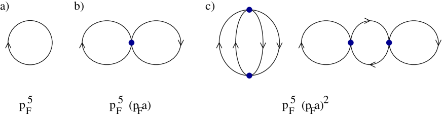
Figure 1: Leading order Feynman diagrams for the ground state energy of a dilute gas of fermions interacting via a short range potential.

There is a formal resemblance between the partition function equ. (3) and the quantum mechanical time evolution operator $U=\exp(-iHt)$. In order to write the partition function as a time evolution operator we have to identify $\beta\to it$ and add the term $-\mu N$ to the Hamiltonian. Using standard techniques we can write the time evolution operators as a path integral Kapusta:1989 ; LeBellac:1996

$$Z=\int D\psi D\psi^{\dagger}\exp\left(-\int_{0}^{\beta}d\tau\int d^{3}x\,{\cal L}_{E}\right).$$ (4)

Here, ${\cal L}_{E}$ is the euclidean lagrangian

$${\cal L}_{E}=\psi^{\dagger}\left(\partial_{\tau}-\mu-\frac{\nabla^{2}}{2m}\right)\psi+\frac{C_{0}}{2}\left(\psi^{\dagger}\psi\right)^{2}.$$ (5)

The fermion fields satisfy anti-periodic boundary conditions $\psi(\beta)=-\psi(0)$. Equation (5) is the starting point of the imaginary time formalism in thermal field theory. The chemical potential simply results in an extra term $-\mu\psi^{\dagger}\psi$ in the lagrangian. From equ. (5) we can easily read off the free fermion propagator

$$S_{\alpha\beta}^{0}(p)=\frac{\delta_{\alpha\beta}}{ip_{4}+\mu-\frac{\vec{p}^{\,2}}{2m}},$$ (6)

where $\alpha,\beta$ are spin labels. We observe that the chemical potential simply shifts the four-component of the momentum. This implies that we have to carefully analyze the boundary conditions in the path integral in order to fix the pole prescription. The correct Minkowski space propagator is

$$S^{0}_{\alpha\beta}(p)=\frac{\delta_{\alpha\beta}}{p_{0}-\epsilon_{p}+i\delta{\rm sgn}(\epsilon_{p})}=\delta_{\alpha\beta}\left\{\frac{\Theta(p-p_{F})}{p_{0}-\epsilon_{p}+i\delta}+\frac{\Theta(p_{F}-p)}{p_{0}-\epsilon_{p}-i\delta}\right\},$$

where $\epsilon_{p}=E_{p}-\mu$, $E_{p}=\vec{p}^{\,2}/(2m)$ and $\delta\to 0^{+}$. The quantity $p_{F}=\sqrt{2m\mu}$ is called the Fermi momentum. We will refer to the surface defined by the condition $|\vec{p}|=p_{F}$ as the Fermi surface. The two terms in equ. (II.1) have a simple physical interpretation. At finite density and zero temperature all states with momenta below the Fermi momentum are occupied, while all states above the Fermi momentum are empty. The possible excitation of the system are particles above the Fermi surface or holes below the Fermi surface, corresponding to the first and second term in equ. (II.1). The particle density is given by

$$\rho=\langle\psi^{\dagger}\psi\rangle=\int\frac{d^{4}p}{(2\pi)^{4}}S^{0}_{\alpha\alpha}(p)\left.e^{ip_{0}\eta}\right|_{\eta\to 0^{+}}=2\int\frac{d^{3}p}{(2\pi)^{3}}\Theta(p_{F}-p)=\frac{p_{F}^{3}}{3\pi^{2}}.$$ (7)

As a first simple application we can compute the energy density as a function of the fermion density. For free fermions, we find

$${\cal E}=2\int\frac{d^{3}p}{(2\pi)^{3}}E_{p}\Theta(p_{F}-p)=\frac{3}{5}\rho\frac{p_{F}^{2}}{2m}.$$ (8)

We can also compute the corrections to the ground state energy due to the interaction $\frac{1}{4}C_{0}(\psi^{\dagger}\psi)^{2}$. The first term is a two-loop diagram with one insertion of $C_{0}$, see Fig. 1. We have

$${\cal E}_{1}=C_{0}\left(\frac{p_{F}^{3}}{6\pi^{2}}\right)^{2}.$$ (9)

We should note that equ. (9) contains two possible contractions, usually called the direct and the exchange term. If the fermions have spin $s$ and degeneracy $g=(2s+1)$ then equ. (9) has to be multiplied by a factor $g(g-1)/2$. We also note that the sum of the first two terms in the energy density can be written as

$${\cal E}=\rho\frac{p_{F}^{2}}{2m}\left(\frac{3}{5}+\frac{2}{3\pi}(p_{F}a)+\ldots\right),$$ (10)

which shows that the $C_{0}$ term is the first term in an expansion in $p_{F}a$, suitable for a dilute, weakly interacting, Fermi gas. The expansion in $(p_{F}a)$ was carried out to order $(p_{F}a)^{2}$ by Huang, Lee and Yang Lee:1957 ; Huang:1957 . Since then, the accuracy was pushed to $O((p_{F}a)^{4}\log(p_{F}a))$ Fetter:1971 , see Hammer:2000xg for a modern perspective. The effective lagrangian can also be used to study many other properties of the system, such as corrections to the fermion propagator. Near the Fermi surface the propagator can be written as

$$S_{\alpha\beta}=\frac{Z\delta_{\alpha\beta}}{p_{0}-v_{F}(|\vec{p}|-p_{F})+i\delta{\rm sgn}(|\vec{p}|-p_{F})},$$ (11)

where $Z$ is the wave function renormalization and $v_{F}=p_{F}/m^{*}$ is the Fermi velocity. $Z$ and $m^{*}$ can be worked out order by order in $(p_{F}a)$, see Abrikosov:1963 ; Platter:2002yr . The main observation is that the structure of the propagator is unchanged even if interactions are taken into account. The low energy excitations are quasi-particles and holes, and near the Fermi surface the lifetime of a quasi-particle is infinite. This is the basis of Fermi liquid theory, see Sec. II. We should note, however, that for nuclear systems the $(p_{F}a)$ expansion is not particularly useful since the nucleon-nucleon scattering length is very large. Equ. (10) is of interest for trapped dilute Fermi gases.

Figure 2: Leading order Feynman diagrams that contribute to the photon polarization function in a non-relativistic Fermi liquid. The tadpole diagram shown in the right panel only appears in the spatial part of the polarization tensor.

II.2 Screening and damping

An important aspect of the dilute Fermi gas is the response to an external electromagnetic field. As a simple example we will consider the case of an a static electric field. The coupling of the gauge field is given by $eA_{0}\psi^{\dagger}\psi$. The medium correction to the photon propagator is determined by the polarization function

$$\Pi_{00}(q)=e^{2}\int d^{4}x\,e^{-iqx}\langle\psi^{\dagger}\psi(0)\psi^{\dagger}\psi(x)\rangle.$$ (12)

The one-loop contribution is given by

$$\Pi_{00}(q)=e^{2}\int\frac{d^{4}p}{(2\pi)^{4}}\frac{1}{q_{0}+p_{0}-\epsilon_{p+q}+i\delta{\rm sgn}(\epsilon_{p+q})}\frac{1}{p_{0}-\epsilon_{p}+i\delta{\rm sgn}(\epsilon_{p})}.$$ (13)

Performing the $p_{0}$ integration by picking up the pole we find

$$\Pi_{00}(q)=e^{2}\int\frac{d^{3}p}{(2\pi)^{3}}\frac{n_{p+q}-n_{p}}{E_{p+q}-E_{p}},$$ (14)

where we have introduced the Fermi distribution function $n_{p}=\Theta(p_{F}-p)$. We observe that in the limit $\vec{q}\to 0$ the polarization function only receives contributions from particle-hole pairs that are closer and closer to the Fermi surface. On the other hand, the energy denominator diverges in this limit because the photon can excite particle-hole pairs with arbitrarily small energy. As a result we get a finite contribution

$$\Pi_{00}(q_{0}=0,\vec{q}\to 0)=e^{2}\int\frac{d^{3}p}{(2\pi)^{3}}\frac{\partial n_{p}}{\partial E_{p}}=e^{2}\frac{p_{F}m}{2\pi^{2}},$$ (15)

which is proportional to the density of states on the Fermi surface. Equ. (15) implies that the static photon propagator in the limit $\vec{q}\to 0$ is modified according to $1/\vec{q}^{\,2}\to 1/(\vec{q}^{\,2}+m_{D}^{2})$, where

$$m_{D}^{2}=e^{2}\left(\frac{p_{F}m}{2\pi^{2}}\right)$$ (16)

is called the Debye mass. The factor $N=(p_{F}m)/(2\pi^{2})$ is equal to the density of states on the Fermi surface. In a relativistic theory we find the same result as in equ. (16) with the density of states replaced by the correct relativistic expression $N=(p_{F}E_{F})/(2\pi^{2})$. The Coulomb potential is modified as

$$V(r)=-e\frac{e^{-r/r_{D}}}{r},$$ (17)

where $r_{D}=1/m_{D}$ is called the Debye screening length. The physics of screening is very easy to understand. A test charge can polarize virtual particle-hole pairs that act to shield the charge.

In the same fashion we can study the response to an external vector potential $\vec{A}$. The coupling of a non-relativistic fermion to the vector potential is determined in the usual way by replacing $\vec{p}\to\vec{p}+e\vec{A}$. Since the kinetic energy operator is quadratic in the momentum we find a linear and a quadratic coupling of the vector potential. The one-loop diagrams that contribute to the polarization tensor are shown in Fig. 2. In the limit of small external momenta we find

$$\Pi_{ij}(q)=e^{2}m_{D}^{2}\int\frac{d\Omega}{4\pi}\left\{v_{i}v_{j}\frac{vk(\hat{q}\cdot\hat{p})}{q_{0}-vk(\hat{q}\cdot\hat{p})}-\frac{1}{3}v^{2}\delta_{ij}\right\},$$ (18)

where $\vec{v}=\vec{p}/m$ is the Fermi velocity. In the limit $q_{0}\!=\!0$ the polarization tensor vanishes. There is no screening of static magnetic fields. For non-zero $q_{0}$ the trace of the polarization tensor is given by

$$\Pi_{ii}(q)=m_{D}^{2}\frac{vq_{0}}{2q}\log\left(\frac{q_{0}-vq}{q_{0}+vq}\right).$$ (19)

The result equ. (19) has an imaginary part if $vq>q_{0}$. This phenomenon is known as Landau damping. The photon is loosing energy to electrons in the Fermi liquid. For a discussion in the context of kinetic theory we refer the reader to Landau:kin .

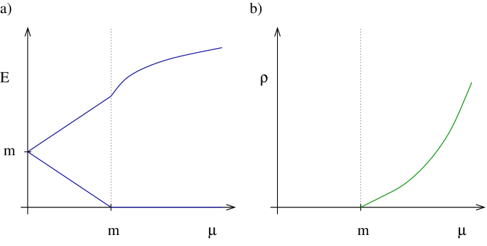
Figure 3: Spectrum and charge density for a charged scalar field as a function of the chemical potential.

III Bose condensation

In this section we introduce some general features of bosonic systems at finite density. We will consider a charged relativistic boson described by the Lagrange density

$${\cal L}_{0}=(\partial^{\mu}\phi^{*})(\partial_{\mu}\phi)-m^{2}\phi^{*}\phi-\lambda(\phi^{*}\phi)^{2}.$$ (20)

Note that $\lambda$ has to be positive in order for the theory to be well defined. This corresponds to a repulsive interaction between the bosons. The lagrangian has a $U(1)$ symmetry $\phi\to e^{-i\varphi}\phi$. The corresponding conserved charge is

$$Q=\int d^{3}x\,i\left(\phi^{*}\partial_{0}\phi-\phi\partial_{0}\phi^{*}\right).$$ (21)

Note that the charge density $\rho$ contains not only the field $\phi$ but also the canonically conjugate momentum $\partial_{0}\phi$. This means that the chemical potential modifies the integration over the canonical momenta in the path integral representation of the partition function. The resulting Minkowski space path integral is Kapusta:1989 ; LeBellac:1996

$$Z=\int D\phi D\phi^{*}\exp\left(i\int d^{4}x{\cal L}\right),$$ (22)

with

$${\cal L}=(\partial_{0}+i\mu)\phi^{*}(\partial_{0}-i\mu)\phi-(\vec{\nabla}\phi^{*})(\vec{\nabla}\phi)-m^{2}\phi^{*}\phi-\lambda(\phi^{*}\phi)^{2}.$$ (23)

There is a simple argument that fixes the form of the lagrangian equ. (23). The argument is based on the observation that we can promote the global $U(1)$ symmetry to a local symmetry by adding a $U(1)$ gauge field to the lagrangian. The charge density is obtained by varying the effective action with respect to the gauge potential. This implies that the chemical potential has to enter the lagrangian like the time component of a gauge field.

We can study the effect of a chemical potential in the mean field approximation. The classical effective potential for the field $\phi$ is given by

$$V(\phi)=(m^{2}-\mu^{2})(\phi^{*}\phi)+\lambda(\phi^{*}\phi)^{2}.$$ (24)

For $\mu>m$ the quadratic term is positive and the minimum of the effective potential is at $\langle\phi\rangle=0$. For $\mu>m$ the origin is unstable and

$$\langle\phi\rangle^{2}=\frac{\mu^{2}-m^{2}}{2\lambda}.$$ (25)

This state is a Bose condensate. The charge density is

$$\rho=\frac{\mu}{\lambda}(\mu^{2}-m^{2}).$$ (26)

In a non-interacting Bose gas the chemical potential cannot be larger than the mass of the boson. In our case, repulsive interactions limit the growth of the density and the chemical potential can take any value. We can also compute the spectrum as a function of the chemical potential. We write $\phi=\langle\phi\rangle+\chi_{1}+i\chi_{2}$ and expand the effective action to second order in $\chi_{1,2}$. For $\mu<m$ we find two modes with energies $E(\vec{p}\!=\!0)=m\pm\mu$. Bose condensation sets in when the lower mode reaches zero energy. Above the onset of Bose condensation we find

$$E_{1}(\vec{p}\!=\!0)=0,\hskip 28.45274ptE_{2}(\vec{p}\!=\!0)=\sqrt{6\mu^{2}-2m^{2}}.$$ (27)

Bose condensation breaks the $U(1)$ symmetry spontaneously and the spectrum contains one Goldstone boson. It is also interesting to study the dispersion relation of the Goldstone mode in more detail. For small momenta we find

$$E_{1}(\vec{p})=\sqrt{1-\frac{2\mu^{2}}{3\mu^{2}-m^{2}}}|\vec{p}|+\ldots.$$ (28)

This shows that at the phase transition point the velocity of the Goldstone mode is zero. Far away from the transition the velocity approaches $v=c/\sqrt{3}$. Bose condensates have many remarkable properties, most notably the fact that they can flow without viscosity. These properties can be derived from the effective action for the Goldstone mode. It was shown, in particular, that this effective action is equivalent to superfluid hydrodynamics popov:1987 ; Son:2002zn .

IV Superconductivity

IV.1 BCS instability

One of the most remarkable phenomena that take place in many body systems is superconductivity. Superconductivity is related to an instability of the Fermi surface in the presence of attractive interactions between fermions. Let us consider fermion-fermion scattering in the simple model introduced in Sect. II. At leading order the scattering amplitude is given by

$$\Gamma_{\alpha\beta\gamma\delta}(p_{1},p_{2},p_{3},p_{4})=C_{0}\left(\delta_{\alpha\gamma}\delta_{\beta\delta}-\delta_{\alpha\delta}\delta_{\beta\gamma}\right).$$ (29)

At next-to-leading order we find the corrections shown in Fig. 4. A detailed discussion of the role of these corrections can be found in Abrikosov:1963 ; Shankar:1993pf ; Polchinski:1992ed . The BCS diagram is special, because in the case of a spherical Fermi surface it can lead to an instability in weak coupling. The main point is that if the incoming momenta satisfy $\vec{p}_{1}\simeq-\vec{p}_{2}$ then there are no kinematic restrictions on the loop momenta. As a consequence, all back-to-back pairs can mix and there is an instability even in weak coupling.

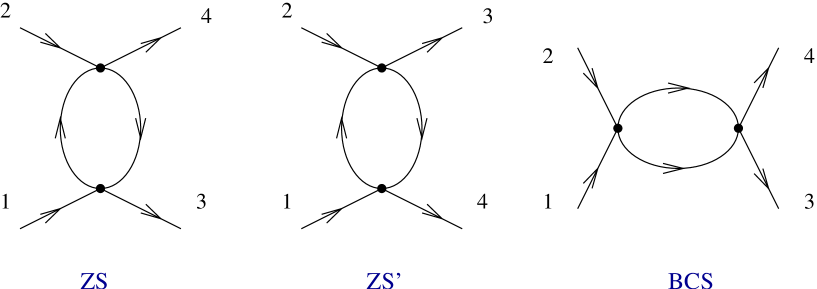
Figure 4: Second order diagrams that contribute to particle-particle scattering. The three diagrams are known as ZS (zero sound), ZS’ and BCS (Bardeen-Cooper-Schrieffer) contribution.

For $\vec{p}_{1}=-\vec{p}_{2}$ and $E_{1}=E_{2}=E$ the BCS diagram is given by

$$\Gamma_{\alpha\beta\gamma\delta}=C_{0}^{2}\left(\delta_{\alpha\gamma}\delta_{\beta\delta}-\delta_{\alpha\delta}\delta_{\beta\gamma}\right)\int\frac{d^{4}q}{(2\pi)^{4}}\frac{1}{E+q_{0}-\epsilon_{q}+i\delta{\rm sgn}(\epsilon_{q})}\frac{1}{E-q_{0}-\epsilon_{q}+i\delta{\rm sgn}(\epsilon_{q})}.$$ (30)

The loop integral has an infrared divergence near the Fermi surface as $E\to 0$. The scattering amplitude is proportional to

$$\Gamma_{\alpha\beta\gamma\delta}=\left(\delta_{\alpha\gamma}\delta_{\beta\delta}-\delta_{\alpha\delta}\delta_{\beta\gamma}\right)\left\{C_{0}-C_{0}^{2}\left(\frac{p_{F}m}{2\pi^{2}}\right)\log\left(\frac{E_{0}}{E}\right)\right\},$$ (31)

where $E_{0}$ is an ultraviolet cutoff. Equ. (31) can be interpreted as an effective energy dependent coupling that satisfies the renormalization group equation Shankar:1993pf ; Polchinski:1992ed

$$E\frac{dC_{0}}{dE}=C_{0}^{2}\left(\frac{p_{F}m}{2\pi^{2}}\right),$$ (32)

with the solution

$$C_{0}(E)=\frac{C_{0}(E_{0})}{1+NC_{0}(E_{0})\log(E_{0}/E)},$$ (33)

where $N=(p_{F}m)/(2\pi^{2})$ is the density of states. Equ. (33) shows that there are two possible scenarios. If the initial coupling is repulsive, $C_{0}(E_{0})>0$, then the renormalization group evolution will drive the effective coupling to zero and the Fermi liquid is stable. If, on the other hand, the initial coupling is attractive, $C_{0}(E_{0})<0$, then the effective coupling grows and reaches a Landau pole at

$$E_{\it crit}\sim E_{0}\exp\left(-\frac{1}{N|C_{0}(E_{0})|}\right).$$ (34)

At the Landau pole the Fermi liquid description has to break down. The renormalization group equation does not determine what happens at this point, but it seems natural to assume that the strong attractive interaction will lead to the formation of a fermion pair condensate. The fermion condensate $\langle\epsilon^{\alpha\beta}\psi_{\alpha}\psi_{\beta}\rangle$ signals the breakdown of the $U(1)$ symmetry and leads to a gap $\Delta$ in the single particle spectrum.

The scale of the gap is determined by the position of the Landau pole, $\Delta\sim E_{\it crit}$. A more quantitative estimate of the gap can be obtained in the mean field approximation. In the path integral formulation the mean field approximation is most easily introduced using the Hubbard-Stratonovich trick. For this purpose we first rewrite the four-fermion interaction as

$$\frac{C_{0}}{2}(\psi^{\dagger}\psi)^{2}=\frac{C_{0}}{4}\left\{(\psi^{\dagger}\sigma_{2}\psi^{\dagger})(\psi\sigma_{2}\psi)+(\psi^{\dagger}\sigma_{2}\vec{\sigma}\psi^{\dagger})(\psi\vec{\sigma}\sigma_{2}\psi)\right\},$$ (35)

where we have used the Fierz identity $2\delta^{\alpha\beta}\delta^{\gamma\rho}=\delta^{\alpha\rho}\delta^{\gamma\beta}+(\vec{\sigma})^{\alpha\rho}(\vec{\sigma})^{\gamma\beta}$. Note that the second term in equ. (35) vanishes because $(\sigma_{2}\vec{\sigma})$ is a symmetric matrix. We now introduce a factor of unity into the path integral

$$1=\frac{1}{Z_{\Delta}}\int D\Delta\exp\left(\frac{\Delta^{*}\Delta}{C_{0}}\right),$$ (36)

where we assume that $C_{0}<0$. We can eliminate the four-fermion term in the lagrangian by a shift in the integration variable $\Delta$. The action is now quadratic in the fermion fields, but it involves a Majorana mass term $\psi\sigma_{2}\Delta\psi+h.c$. The Majorana mass terms can be handled using the Nambu-Gorkov method. We introduce the bispinor $\Psi=(\psi,\psi^{\dagger}\sigma_{2})$ and write the fermionic action as

$${\cal S}=\frac{1}{2}\int\frac{d^{4}p}{(2\pi)^{4}}\Psi^{\dagger}\left(\begin{array}[]{cc}p_{0}-\epsilon_{p}&\Delta\\ \Delta^{*}&p_{0}+\epsilon_{p}\end{array}\right)\Psi.$$ (37)

Since the fermion action is quadratic we can integrate the fermion out and obtain the effective lagrangian

$${\cal L}=\frac{1}{2}{\rm Tr}\left[\log\left(G_{0}^{-1}G\right)\right]+\frac{1}{C_{0}}|\Delta|^{2},$$ (38)

where $G$ is the fermion propagator

$$G(p)=\frac{1}{p_{0}^{2}-\epsilon_{p}^{2}-|\Delta|^{2}}\left(\begin{array}[]{cc}p_{0}+\epsilon_{p}&\Delta^{*}\\ \Delta&p_{0}-\epsilon_{p}\end{array}\right).$$ (39)

The diagonal and off-diagonal components of $G(p)$ are sometimes referred to as normal and anomalous propagators. Note that we have not yet made any approximation. We have converted the fermionic path integral to a bosonic one, albeit with a very non-local action. The mean field approximation corresponds to evaluating the bosonic path integral using the saddle point method. Physically, this approximation means that the order parameter does not fluctuate. Formally, the mean field approximation can be justified in the large $N$ limit, where $N$ is the number of fermion fields. The saddle point equation for $\Delta$ gives the gap equation

$$\Delta=|C_{0}|\int\frac{d^{4}p}{(2\pi)^{4}}\frac{\Delta}{p_{0}^{2}-\epsilon^{2}_{p}-\Delta^{2}}.$$ (40)

Performing the $p_{0}$ integration we find

$$1=\frac{|C_{0}|}{2}\int\frac{d^{3}p}{(2\pi)^{3}}\frac{1}{\sqrt{\epsilon^{2}_{p}+\Delta^{2}}}.$$ (41)

Since $\epsilon_{p}=E_{p}-\mu$ the integral in equ. (41) has an infrared divergence on the Fermi surface $|\vec{p}|\sim p_{F}$. As a result, the gap equation has a non-trivial solution even if the coupling is arbitrarily small. The magnitude of the gap is $\Delta\sim\Lambda\exp(-1/(|C_{0}|N))$ where $\Lambda$ is a cutoff that regularizes the integral in equ. (41) in the ultraviolet. If we treat equ. (1) as a low energy effective field theory we should be able to eliminate the unphysical dependence of the gap on the ultraviolet cutoff, and express the gap in terms of a physical observable. At low density, this can be achieved by observing that the gap equation has the same UV behavior as the Lipmann-Schwinger equation that determines the scattering length at zero density

$$\frac{mC_{0}}{4\pi a}-1=\frac{C_{0}}{2}\int\frac{d^{3}p}{(2\pi)^{3}}\frac{1}{E_{P}}.$$ (42)

Combining equs. (41) and (42) we can derive an UV finite gap equation that depends only on the scattering length,

$$-\frac{m}{4\pi a}=\frac{1}{2}\int\frac{d^{3}p}{(2\pi)^{3}}\Big{\{}\frac{1}{\sqrt{\epsilon^{2}_{p}+\Delta^{2}}}-\frac{1}{E_{p}}\Big{\}}.$$ (43)

A careful analysis gives Papenbrock:1998wb ; Khodel:1996

$$\Delta=\frac{8E_{f}}{e^{2}}\exp\left(-\frac{\pi}{2p_{F}|a|}\right).$$ (44)

For neutron matter the scattering length is large, $a=-18.8$ fm, and equ. (44) is not very useful, except at very small density. Calculations based on potential models give gaps on the order of 2 MeV at nuclear matter density.

In the limit of very high density we can eliminate the cutoff dependence using a method introduced by Weinberg Weinberg:1994 . Weinberg defines a renormalized effective potential and shows that the renormalization scale dependence of the effective potential is canceled by the scale dependence of the coupling. The effective coupling satisfies the renormalization group equ. (32). The gap is determined by the effective coupling at the energy scale $E_{0}$. In practice, this would typically be the energy scale at which the four-fermion interaction is matched against a more microscopic description in terms of meson (nuclear physics) or phonon exchange (condensed matter physics).

IV.2 Fermi liquid, revisited

Our discussion of Fermi liquids in Sect. II and in the previous section was based on the simple model defined in equ. (1). In this section we shall briefly discuss the structure of fermionic many-body systems in the case of more general interactions. We will restrict ourselves to systems that can be described in terms of purely fermionic actions, with all other degrees of freedom integrated out. For more details we refer the reader to Shankar:1993pf .

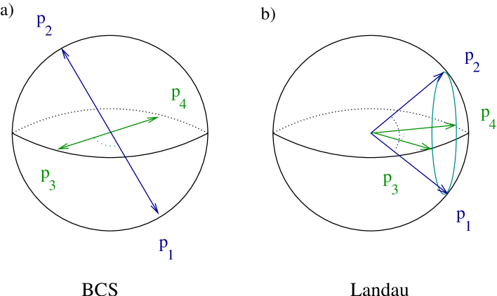
Figure 5: Kinematic configurations for fermion-fermion scattering that correspond to four-fermion operators that are marginal at tree level. The left panel shows BCS (back-to-back) scattering and the right panel shows forward scattering.

We can view the model defined by equ. (1) as an example of an effective field theory, valid for momenta close to the Fermi surface. In order to construct an effective field theory we have to write all possible interactions that are allowed by the symmetries of the theory. The effective action of rotationally invariant, non-relativistic Fermi system is given by

$$S=\int\frac{d^{4}p}{(2\pi)^{4}}\psi(p)^{\dagger}\left(p_{0}-v_{F}l_{p}\right)\psi(p)+\frac{1}{4}\left[\prod_{i=1}^{4}\int\frac{d^{4}p_{i}}{(2\pi)^{4}}\right]\psi^{\dagger}(p_{4})\psi^{\dagger}(p_{3})\psi(p_{2})\psi(p_{1})U(p_{4},p_{3},p_{2},p_{1}),$$ (45)

where $v_{F}=\partial\epsilon_{p}/(\partial p)$ and $l_{p}=|\vec{p}|-p_{F}$. We have suppressed the spin indices of the potential $U$. The power counting for the effective theory can be established by studying the scaling behavior of all allowed operators under transformations of the type $l_{p}\to sl_{p}$ that scale the momenta towards the Fermi surface. Writing $\epsilon_{p}=v_{F}l_{p}+O(l_{p}^{2})$ we see that as $s\to 0$ only the Fermi velocity survives, the detailed form of the dispersion relation is irrelevant. Using this method we can also see that with the exception of special kinematic regimes the four-fermion interaction is irrelevant. We already saw that one exception is provided by the BCS interaction

$$U(-\hat{p}_{3},\hat{p}_{3},-\hat{p}_{1},\hat{p}_{1})=V(\hat{p}_{1}\cdot\hat{p}_{3})=\sum_{l}V_{l}P_{l}(\hat{p}_{1}\cdot\hat{p}_{3}),$$ (46)

where $P_{l}(x)$ are Legendre polynomials. At tree level $V(x)$ is a marginal operator, that means it is invariant under rescaling the momenta towards the Fermi surface. This changes at one-loop level. If any of the couplings $V_{l}$ is attractive then this coupling will grow according to the renormalization group equ. (32) and eventually reach a Landau pole. If there is more than one attractive coupling $V_{l}$ then the ground state is determined by which coupling reaches its Landau pole first. If all $V_{l}$ are repulsive then the BCS potential becomes irrelevant as the evolution approaches the Fermi surface.

In this case there is another kinematic regime that becomes important. We can take any two momenta on the Fermi surface, not necessarily back-to-back, and find an allowed final state. Energy and momentum conservation implies that $\hat{p}_{1}\cdot\hat{p}_{2}=\hat{p}_{3}\cdot\hat{p}_{4}$. In two-dimensions this would restrict the scattering to be either forward or exchange, but in three dimensions there is a circle of allowed final states parametrized by the angle $\phi_{12,34}$ between the planes spanned by the incoming and outgoing momenta, see Fig. 5. The interaction is

$$\left.U(\hat{p}_{4},\hat{p}_{3},\hat{p}_{2},\hat{p}_{1})\right|_{\hat{p}_{1}\cdot\hat{p}_{2}=\hat{p}_{3}\cdot\hat{p}_{4}}=F(\hat{p}_{1}\cdot\hat{p}_{2},\phi_{12,34})$$ (47)

The function $F(x,0)$ is called the Landau function and its Legendre coefficients are referred to as Landau parameters. The Landau parameters remain marginal at one-loop order. A many body system characterized by $v_{F}$ and $F_{l}$ is called a Landau Fermi liquid Pines:1966 ; Baym:1991 . A Landau liquid behaves qualitatively like a dilute, weakly interacting, Fermi liquid, even if the interaction is not weak and the system is not dilute. In particular, the excitations of a Landau liquid are quasi-particles and holes. The Landau parameters encode the quasi-particle interaction and can be used to compute observables like the equation of state and the response to external fields.

One can show that operators involving more than four fermion fields are irrelevant near the Fermi surface. This does not imply that $n>4$ fermion operators play no role at all. For example, if one of the $V_{l}$ has a Landau pole at energy $E_{0}$ then the six fermion interaction still has a finite coupling at this scale and will cause observable effects, see Sec. IX.5 for an example. Also, just because the $V_{l}$ are the only operators that cause instabilities in weak coupling does not imply that other operators cannot have instabilities in strong coupling. For example, dilute nuclear matter may have a phase characterized by alpha particle condensation rather than superconductivity.

IV.3 Landau-Ginzburg theory

In this section we shall study the properties of a superconductor in more detail. For definiteness, we will consider a system of electrons coupled to a $U(1)$ gauge field $A_{\mu}$. The order parameter $\Phi=\langle\epsilon^{\alpha\beta}\psi_{\alpha}\psi_{\beta}\rangle$ breaks $U(1)$ invariance. Consider a gauge transformation

$$A_{\mu}\to A_{\mu}+\partial_{\mu}\Lambda.$$ (48)

The order parameter transforms as

$$\Phi\to\exp(2ie\Lambda)\Phi.$$ (49)

The breaking of gauge invariance is responsible for most of the unusual properties of superconductors Anderson:1984 ; Weinberg:1995 . This can be seen by constructing the low energy effective action of a superconductor. For this purpose we write the order parameter in terms of its modulus and phase

$$\Phi(x)=\exp(2ie\phi(x))\tilde{\Phi}(x).$$ (50)

The field $\phi$ corresponds to the Goldstone mode. Under a gauge transformation $\phi(x)\to\phi(x)+\Lambda(x)$. Gauge invariance restricts the form of the effective Lagrange function as

$$L=-\frac{1}{4}\int d^{3}x\,F_{\mu\nu}F_{\mu\nu}+L_{s}(A_{\mu}-\partial_{\mu}\phi).$$ (51)

There is a large amount of information we can extract even without knowing the explicit form of $L_{s}$. Stability implies that $A_{\mu}=\partial_{\mu}\phi$ corresponds to a minimum of the energy. This means that up to boundary effects the gauge potential is a total divergence and that the magnetic field has to vanish. This phenomenon is known as the Meissner effect.

Equ. (51) also implies that a superconductor has zero resistance. The equations of motion relate the time dependence of the Goldstone boson field to the potential,

$$\dot{\phi}(x)=-V(x).$$ (52)

The electric current is related to the gradient of the Goldstone boson field. Equ. (52) shows that the time dependence of the current is proportional to the gradient of the potential. In order to have a static current the gradient of the potential has to be constant throughout the sample, and the resistance is zero.

In order to study the properties of a superconductor in more detail we have to specify $L_{s}$. For this purpose we assume that the system is time-independent, that the spatial gradients are small, and that the order parameter is small. In this case we can write

$$L_{s}=\int d^{3}x\,\left\{-\frac{1}{2}\left|\left(\nabla-2ie\vec{A}\right)\Phi\right|^{2}+\frac{1}{2}m^{2}_{H}\left(\Phi^{*}\Phi\right)^{2}-\frac{1}{4}g\left(\Phi^{*}\Phi\right)^{4}+\ldots\right\},$$ (53)

where $m_{H}$ and $g$ are unknown parameters that depend on the temperature. Equ. (53) is known as the Landau-Ginzburg effective action. Strictly speaking, the assumption that the order parameter is small can only be justified in the vicinity of a second order phase transition. Nevertheless, the Landau-Ginzburg description is instructive even in the regime where $t=(T-T_{c})/T_{c}$ is not small. It is useful to decompose $\Phi=\rho\exp(2ie\phi)$. For constant fields the effective potential,

$$V(\rho)=-\frac{1}{2}m_{H}^{2}\rho^{2}+\frac{1}{4}g\rho^{4},$$ (54)

is independent of $\phi$. The minimum is at $\rho_{0}^{2}=m_{H}^{2}/g$ and the energy density at the minimum is given by ${\cal E}=-m_{H}^{4}/(4g)$. This shows that the two parameters $m_{H}$ and $g$ can be related to the expectation value of $\Phi$ and the condensation energy. We also observe that the phase transition is characterized by $m_{H}(T_{c})=0$.

In terms of $\phi$ and $\rho$ the Landau-Ginzburg action is given by

$$L_{s}=\int d^{3}x\,\left\{-2e^{2}\rho^{2}\left(\vec{\nabla}\phi-\vec{A}\right)^{2}+\frac{1}{2}m_{H}^{2}\rho^{2}-\frac{1}{4}g\rho^{4}-\frac{1}{2}\left(\nabla\rho\right)^{2}\right\}.$$ (55)

The equations of motion for $\vec{A}$ and $\rho$ are given by

$$\vec{\nabla}\times\vec{B} = 4e^{2}\rho^{2}\left(\nabla\phi-\vec{A}\right),$$ (56)

$$\nabla^{2}\rho = -m_{H}^{2}\rho^{2}+g\rho^{3}+4e^{2}\rho\left(\vec{\nabla}\phi-\vec{A}\right).$$ (57)

Equ. (56) implies that $\nabla^{2}\vec{B}=-4e^{2}\rho^{2}\vec{B}$. This means that an external magnetic field $\vec{B}$ decays over a characteristic distance $\lambda=1/(2e\rho)$. Equ. (57) gives $\nabla^{2}\rho=-m_{H}^{2}\rho+\ldots$. As a consequence, variations in the order parameter relax over a length scale given by $\xi=1/m_{H}$. The two parameters $\lambda$ and $\xi$ are known as the penetration depth and the coherence length.

The relative size of $\lambda$ and $\xi$ has important consequences for the properties of superconductors. In a type II superconductor $\xi<\lambda$. In this case magnetic flux can penetrate the system in the form of vortex lines. At the core of a vortex the order parameter vanishes, $\rho=0$. In a type II material the core is much smaller than the region over which the magnetic field goes to zero. The magnetic flux is given by

$$\int_{A}\vec{B}\cdot\vec{S}=\oint_{\partial A}\vec{A}\cdot d\vec{l}=\oint_{\partial A}\vec{\nabla}\phi\cdot d\vec{l}=\frac{n\pi\hbar}{e},$$ (58)

and quantized in units of $\pi\hbar/e$. In a type II superconductor magnetic vortices repel each other and form a regular lattice known as the Abrikosov lattice. In a type I material, on the other hand, vortices are not stable and magnetic fields can only penetrate the sample if superconductivity is destroyed.

The Landau-Ginzburg description shows that there is no qualitative difference between superconductivity and Bose condensation of charged bosons. Indeed, we may think of superconductivity as Bose condensation of Cooper pairs. While this is qualitatively correct, there is an important quantitative difference between a BCS superconductor and a dilute Bose condensate of composite bosons. In a BCS superconductor the coherence length $\xi$, which is a measure of the size of the Cooper pairs, is much larger than the average inter-particle spacing $p_{F}^{-1}$. Also, the pair correlation essentially disappears above the critical temperature. In a dilute Bose condensate, on the other hand, the size of the bosons is much smaller than the typical distance between them. The bosons are tightly bound and do not dissolve at $T_{c}$. Nevertheless, since there is no qualitative difference between Bose condensation and BCS superconductivity we expect to find systems that show a crossover from one kind of behavior to the other. We will discuss an example in Sect. VIII.4.

V QCD and symmetries

Before we discuss QCD at finite baryon density we would like to provide a quick reminder on QCD and the symmetries of QCD. The elementary degrees of freedom are quark fields $\psi^{a}_{\alpha,f}$ and gluons $A_{\mu}^{a}$. Here, $a$ is color index that transforms in the fundamental representation for fermions and in the adjoint representation for gluons. Also, $f$ labels the quark flavors $u,d,s,c,b,t$. In practice, we will focus on the three light flavors up, down and strange. The QCD lagrangian is

$${\cal L}=\sum_{f}^{N_{f}}\bar{\psi}_{f}(iD/\,-m_{f})\psi_{f}-\frac{1}{4}G_{\mu\nu}^{a}G_{\mu\nu}^{a},$$ (59)

where the field strength tensor is defined by

$$G_{\mu\nu}^{a}=\partial_{\mu}A_{\nu}^{a}-\partial_{\nu}A_{\mu}^{a}+gf^{abc}A_{\mu}^{b}A_{\nu}^{c},$$ (60)

and the covariant derivative acting on quark fields is

$$iD/\,\psi=\gamma^{\mu}\left(i\partial_{\mu}+gA_{\mu}^{a}\frac{\lambda^{a}}{2}\right)\psi.$$ (61)

QCD has a number of remarkable properties. Most remarkably, even though QCD accounts for the rich phenomenology of hadronic and nuclear physics, it is an essentially parameter free theory. To first approximation, the masses of the light quarks $u,d,s$ are too small to be important, while the masses of the heavy quarks $c,b,t$ are too heavy. If we set the masses of the light quarks to zero and take the masses of the heavy quarks to be infinite then the only parameter in the QCD lagrangian is the coupling constant, $g$. Once quantum corrections are taken into account $g$ becomes a function of the scale at which it is measured. If the scale is large then the coupling is small, but in the infrared the coupling becomes large. This is the famous phenomenon of asymptotic freedom. Since the coupling depends on the scale the dimensionless parameter $g$ is traded for a dimensionful scale parameter $\Lambda_{QCD}$. In essence, $\Lambda_{QCD}$ is the scale at which the coupling becomes large.

Since $\Lambda_{QCD}$ is the only dimensionful quantity in QCD ($m_{q}=0$) it is not really a parameter of QCD, but reflects our choice of units. In standard units, $\Lambda_{QCD}\simeq 200\,{\rm MeV}\simeq 1\,{\rm fm}^{-1}$. Note that hadrons indeed have sizes $r\sim\Lambda_{QCD}^{-1}$. However, we should also note that in practice the perturbative expansion in $g$ breaks down at scales $r\sim\Lambda_{\chi SB}^{-1}\sim 0.2\,{\rm fm}\ll\Lambda_{QCD}^{-1}$.

Another important feature of the QCD lagrangian are its symmetries. First of all, the lagrangian is invariant under local gauge transformations $U(x)\in SU(3)_{c}$

$$\psi(x)\to U(x)\psi(x),\hskip 28.45274ptA_{\mu}(x)\to U(x)A_{\mu}U^{\dagger}(x)+iU(x)\partial_{\mu}U^{\dagger}(x),$$ (62)

where $A_{\mu}=A_{\mu}^{a}(\lambda^{a}/2)$. In the QCD ground state at zero temperature and density the local color symmetry is confined. This implies that all excitations are singlets under the gauge group.

The dynamics of QCD is completely independent of flavor. This implies that if the masses of the quarks are equal, $m_{u}=m_{d}=m_{s}$, then the theory is invariant under arbitrary flavor rotations of the quark fields

$$\psi_{f}\to V_{fg}\psi_{g},$$ (63)

where $V\in SU(3)$. This is the well known flavor (isospin) symmetry of the strong interactions. If the quark masses are not just equal, but equal to zero, then the flavor symmetry is enlarged. This can be seen by defining left and right-handed fields

$$\psi_{L,R}=\frac{1}{2}(1\pm\gamma_{5})\psi.$$ (64)

In terms of $L/R$ fields the fermionic lagrangian is

$${\cal L}=\bar{\psi}_{L}(iD/\,)\psi_{L}+\bar{\psi}_{R}(iD/\,)\psi_{R}+\bar{\psi}_{L}M\psi_{R}+\bar{\psi}_{R}M\psi_{L},$$ (65)

where $M={\rm diag}(m_{u},m_{d},m_{s})$. We observe that if quarks are massless, $m_{u}=m_{d}=m_{s}=0$, then there is no coupling between left and right handed fields. As a consequence, the lagrangian is invariant under independent flavor transformations of the left and right handed fields.

$$\psi_{L,f}\to L_{fg}\psi_{L,g},\hskip 28.45274pt\psi_{R,f}\to R_{fg}\psi_{R,g},$$ (66)

where $(L,R)\in SU(3)_{L}\times SU(3)_{R}$. In the real world, of course, the masses of the up, down and strange quarks are not zero. Nevertheless, since $m_{u},m_{d}\ll m_{s}<\Lambda_{QCD}$ QCD has an approximate chiral symmetry.

In the QCD ground state at zero temperature and density the flavor symmetry is realized, but the chiral symmetry is spontaneously broken by a quark-anti-quark condensate $\langle\bar{\psi}_{L}\psi_{R}+\bar{\psi}_{R}\psi_{L}\rangle$. As a result, the observed hadrons can be approximately assigned to representations of the $SU(3)_{V}$ flavor group, but not to representations of $SU(3)_{L}\times SU(3)_{R}$. Nevertheless, chiral symmetry has important implications for the dynamics of QCD at low energy. Goldstone’s theorem implies that the breaking of $SU(3)_{L}\times SU(3)_{R}\to SU(3)_{V}$ is associated with the appearance of an octet of (approximately) massless pseudoscalar Goldstone bosons. Chiral symmetry places important restrictions on the interaction of the Goldstone bosons. These constraints are obtained most easily from the low energy effective chiral lagrangian. At leading order we have

$${\cal L}=\frac{f_{\pi}^{2}}{4}{\rm Tr}\left[\partial_{\mu}\Sigma\partial^{\mu}\Sigma^{\dagger}\right]+\Big{[}B{\rm Tr}(M\Sigma^{\dagger})+h.c.\Big{]}+\ldots,$$ (67)

where $\Sigma=\exp(i\phi^{a}\lambda^{a}/f_{\pi})$ is the chiral field, $f_{\pi}$ is the pion decay constant and $M$ is the mass matrix. Expanding $\Sigma$ in powers of the pion, kaon and eta fields $\phi^{a}$ we can derive the leading order chiral perturbation theory results for Goldstone boson scattering and the coupling of Goldstone bosons to external fields. Higher order corrections originate from loops and higher order terms in the effective lagrangian.

Finally, we observe that the QCD lagrangian has two $U(1)$ symmetries,

$$U(1)_{B}:\hskip 28.45274pt \psi_{L}\to e^{i\phi}\psi_{L},\hskip 28.45274pt \psi_{R}\to e^{i\phi}\psi_{R}$$ (68)

$$U(1)_{A}:\hskip 28.45274pt \psi_{L}\to e^{i\alpha}\psi_{L},\hskip 28.45274pt \psi_{R}\to e^{-i\alpha}\psi_{R}.$$ (69)

The $U(1)_{B}$ symmetry is exact even if the quarks are not massless. Superficially, it appears that the $U(1)_{A}$ symmetry is explicitly broken by the quark masses and spontaneously broken by the quark condensate. However, there is no Goldstone boson associated with spontaneous $U(1)_{A}$ breaking. The reason is that at the quantum level the $U(1)_{A}$ symmetry is broken by an anomaly. The divergence of the $U(1)_{A}$ current is given by

$$\partial^{\mu}j_{\mu}^{5}=\frac{N_{f}g^{2}}{16\pi^{2}}G^{a}_{\mu\nu}\tilde{G}^{a}_{\mu\nu},$$ (70)

where $\tilde{G}^{a}_{\mu\nu}=\epsilon_{\mu\nu\alpha\beta}G^{a}_{\alpha\beta}/2$ is the dual field strength tensor.

VI QCD at finite density

In the real world the quark masses are not equal and the only exact global symmetries of QCD are the $U(1)_{f}$ flavor symmetries associated with the conservation of the number of up, down, and strange quarks. If we take into account the weak interactions then flavor is no longer conserved and the only exact symmetries are the $U(1)_{B}$ of baryon number and the $U(1)_{Q}$ of electric charge.

In the following we study hadronic matter at non-zero baryon density. We will mostly focus on systems at non-zero baryon chemical potential but zero electron $U(1)_{Q}$ chemical potential. We should note that in the context of neutron stars we are interested in situations when the electric charge, but not necessarily the electron chemical potential, is zero. We will comment on the consequences of electric charge neutrality below. Also, if the system is in equilibrium with respect to strong, but not to weak interactions, then non-zero flavor chemical potentials may come into play.

The partition function of QCD at non-zero baryon chemical potential is given by

$$Z=\sum_{i}\exp\left(-\frac{E_{i}-\mu N_{i}}{T}\right),$$ (71)

where $i$ labels all quantum states of the system, $E_{i}$ and $N_{i}$ are the energy and baryon number of the state $i$. If the temperature and chemical potential are both zero then only the ground state contributes to the partition function. All other states give contributions that are exponentially small if the volume of the system is taken to infinity. In QCD there is a massgap for states that carry baryon number. As a a consequence there is an onset chemical potential

$$\mu_{\it onset}=\min_{i}(E_{i}/N_{i}),$$ (72)

such that the partition function is independent of $\mu$ for $\mu<\mu_{\it onset}$. For $\mu>\mu_{\it onset}$ the baryon density is non-zero. If the chemical potential is just above the onset chemical potential we can describe QCD, to first approximation, as a dilute gas of non-interacting nucleons. In this approximation $\mu_{\it onset}=m_{N}$. Of course, the interaction between nucleons is essential. Without it, we would not have stable nuclei. As a consequence, nuclear matter is self-bound and the energy per baryon in the ground state is given by

$$\frac{E_{N}}{N}-m_{N}\simeq-15\,{\rm MeV}.$$ (73)

The onset transition is a first order transition at which the baryon density jumps from zero to nuclear matter saturation density, $\rho_{0}\simeq 0.14\,{\rm fm}^{-3}$. The first order transition continues into the finite temperature plane and ends at a critical endpoint at $T=T_{c}\simeq 10$ MeV, see Fig. 6.

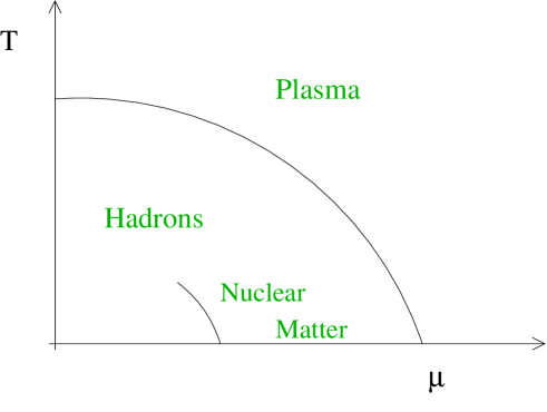
Figure 6: Naive phase diagram of hadronic matter as a function of the baryon chemical potential and temperature.

Nuclear matter is a complicated many-body system and, unlike the situation at zero density and finite temperature, there is also no information from numerical simulations on the lattice. This is related to the so-called ’sign problem’. At non-zero chemical potential the euclidean fermion determinant is complex and standard Monte-Carlo techniques based on importance sampling fail. Recently, some progress has been made in simulating QCD for small $\mu$ and $T\simeq T_{c}$ Fodor:2001pe ; deForcrand:2002ci ; Allton:2002zi , but the regime of small temperature remains inaccessible. As a consequence of the sign problem, there are also essentially no general results concerning the structure of the ground state. While the theorems of Vafa and Witten Vafa:tf ; Vafa:1984xg rule out spontaneous breaking of parity or flavor at $T\neq 0$ and $\mu=0$, there are no theorems of this type at non-zero baryon density.

However, if the density is very much larger than nuclear matter saturation density, $\rho\gg\rho_{0}$, we expect the problem to simplify. In this regime it is natural to use a system of non-interacting quarks as a starting point Collins:1974ky . The low energy degrees of freedom are quark excitations and holes in the vicinity of the Fermi surface. Since the Fermi momentum is large, asymptotic freedom implies that the interaction between quasi-particles is weak. As a consequence, the naive expectation is that chiral symmetry is restored and quarks and gluons are deconfined. It seems natural to assume that the quark liquid at high baryon density is continuously connected to the quark-gluon plasma at high temperature. These naive expectations are summarized in the phase diagram shown in Fig. 6.

Corrections to the non-interacting quark liquid can be studied in perturbation theory. The thermodynamic potential is given by Freedman:1976xs ; Fraga:2001id

$$\Omega(\mu)=-\frac{N_{f}\mu^{4}}{4\pi^{2}}\left\{1-2\left(\frac{\alpha_{s}}{\pi}\right)-\left[G+N_{f}\log\left(\frac{\alpha_{s}}{\pi}\right)+\left(11-\frac{2}{3}N_{f}\right)\log\left(\frac{\bar{\Lambda}}{\mu}\right)\right]\left(\frac{\alpha_{s}}{\pi}\right)^{2}\right\}\;,$$ (74)

where $G=G_{0}-0.536N_{f}+N_{f}\ln{N_{f}}$, $G_{0}=10.374\pm 0.13$. Here, $\mu$ is the chemical potential for quark number. This convention is more natural in the context of perturbative QCD and we will use it for the remainder of these lectures. Note that perturbative corrections reduce the pressure of the quark phase. At least qualitatively, this is agreement with the idea that at very low density the pressure of the hadron phase is bigger than the pressure of the quark phase.

VII Color superconductivity

There are two problems with the perturbative expansion equ. (74). One problem is related to the fact that while the electric gluon interaction is screened by the mechanism discussed in Sect. II.2 there is no screening of magnetic gluon exchanges. This not only implies that the magnetic sector of the theory becomes non-perturbative, it also causes the Fermi liquid description to break down Holstein:1973 ; Reizer:1989 . The correction to the fermion self energy near the Fermi surface due to magnetic gluon exchanges is Baym:uj ; Manuel:2000nh ; Boyanovsky:2000bc ; Brown:1999yd

$$\Sigma_{0}(p_{0})=\frac{g^{2}}{9\pi^{2}}\log\left(\frac{\mu}{p_{0}}\right).$$ (75)

This correction invalidates the Fermi liquid description for energies $p_{0}\sim\mu\exp(-1/g^{2})$. But even before this phenomenon becomes important there is another effect that will invalidate the Fermi liquid picture. In Sect. IV.1 we showed that the BCS instability will lead to pair condensation whenever there is an attractive fermion-fermion interaction. At very large density, the attraction is provided by one-gluon exchange between quarks in a color anti-symmetric $\bar{3}$ state. High density quark matter is therefore expected to behave as a color superconductor Frau_78 ; Barrois:1977xd ; Bar_79 ; Bailin:1984bm .

Color superconductivity is described by a pair condensate of the form

$$\Phi=\langle\psi^{T}C\Gamma_{D}\lambda_{C}\tau_{F}\psi\rangle.$$ (76)

Here, $C$ is the charge conjugation matrix, and $\Gamma_{D},\lambda_{C},\tau_{F}$ are Dirac, color, and flavor matrices. Except in the case of only two colors, the order parameter cannot be a color singlet. Color superconductivity is therefore characterized by the breakdown of color gauge invariance. This statement has to be interpreted in the sense of Sect. IV.3. Gluons acquire a mass due to the (Meissner-Anderson) Higgs mechanism.

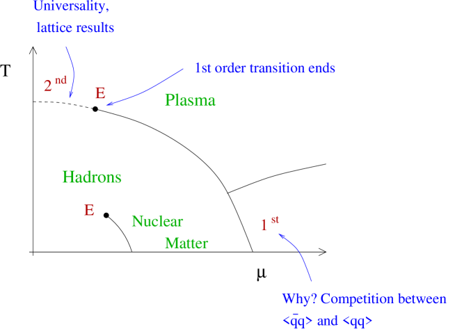
Figure 7: First revision of the phase diagram of hadronic matter. This figure shows the phase diagram of strongly interacting matter obtained from a mean field treatment of chiral symmetry breaking and color superconductivity in QCD with two flavors, see e.g. Berges:1998 .

A rough estimate of the critical density for the transition from chiral symmetry breaking to color superconductivity, the superconducting gap and the transition temperature is provided by schematic four-fermion models Alford:1998zt ; Rapp:1998zu . Typical models are based on the instanton interaction

$${\cal L}=G_{I}\left\{(\bar{\psi}\tau^{-}_{\alpha}\psi)^{2}+(\bar{\psi}\gamma_{5}\tau^{-}_{\alpha}\psi)^{2}\right\},$$ (77)

or a schematic one-gluon exchange interaction

$${\cal L}=G_{OGE}\left(\bar{\psi}\gamma_{\mu}\frac{\lambda^{a}}{2}\psi\right)^{2}.$$ (78)

Here $\tau^{-}_{\alpha}=(\vec{\tau},i)$ is an isospin matrix and $\lambda^{a}$ are the color Gell-Mann matrices. The strength of the four-fermion interaction is typically tuned to reproduce the magnitude of the chiral condensate and the pion decay constant at zero temperature and density. In the mean field approximation the effective quark mass associated with chiral symmetry breaking is determined by a gap equation of the type

$$M_{Q}=G_{M}\int^{\Lambda}\frac{d^{3}p}{(2\pi)^{3}}\frac{M_{Q}}{\sqrt{{\vec{p}}^{\,2}+M_{Q}^{2}}}\left(1-n_{F}(E_{p})\right),$$ (79)

where $G_{M}$ is the effective coupling in the quark-anti-quark channel and $\Lambda$ is a cutoff. Both the instanton interaction and the one-gluon exchange interaction are attractive in the color anti-triplet scalar diquark channel $\epsilon^{abc}(\psi^{b}C\gamma_{5}\psi^{c})$. A pure one-gluon exchange interaction leads to a degeneracy between scalar and pseudoscalar diquark condensation, but instantons are repulsive in the pseudoscalar diquark channel. The gap equation in the scalar diquark channel is

$$\Delta=\frac{G_{D}}{2}\int^{\Lambda}\frac{d^{3}p}{(2\pi)^{3}}\frac{\Delta}{\sqrt{(|\vec{p}|-p_{F})^{2}+\Delta^{2}}},$$ (80)

where we have neglected terms that do not have a singularity on the Fermi surface, $|\vec{p}|=p_{F}$. In the case of a four-fermion interaction with the quantum numbers of one-gluon exchange $G_{D}=G_{M}/(N_{c}-1)$. The same result holds for instanton effects. In order to determine the correct ground state we have to compare the condensation energy in the chiral symmetry broken and diquark condensed phases. We have ${\cal E}\sim f_{\pi}^{2}M_{Q}^{2}$ in the $(\bar{q}q)$ condensed phase and ${\cal E}\sim p_{F}^{2}\Delta^{2}/(2\pi^{2})$ in the $(qq)$ condensed phase.

At zero temperature and density both equs. (79) and (80) only have non-trivial solutions if the coupling exceeds a critical value. Since $G_{M}>G_{D}$ we have $M_{Q}>\Delta$ and the energetically preferred solution corresponds to chiral symmetry breaking. If the density increases Pauli-Blocking in equ. (79) becomes important and the effective quark mass decreases. The diquark gap equation behaves very differently. Equ. (80) has an infrared singularity on the Fermi surface, $p=p_{F}$, and this singularity is multiplied by a finite density of states, $N=p_{F}^{2}/(2\pi)^{2}$. As a consequence, there is a non-trivial solution even if the coupling is weak. The gap grows with density until the Fermi momentum becomes on the order of the cutoff. For realistic values of the parameters we find a first order transition for remarkably small values of the quark chemical potential, $\mu_{Q}\simeq 300$ MeV. The gap in the diquark condensed phase is $\Delta\sim 100$ MeV and the critical temperature is $T_{c}\sim 50$ MeV.

In the same model the finite temperature phase transition at zero baryon density is found to be of second order. This result is in agreement with universality arguments Pisarski:ms and lattice results. If the transition at finite density and zero temperature is indeed of first order then the first order transition at zero baryon density has to end in a tri-critical point Barducci:1989wi ; Barducci:1989eu ; Barducci:1993bh ; Berges:1998 ; Halasz:1998 . The tri-critical point is quite remarkable, because it remains a true critical point, even if the quark masses are not zero. A non-zero quark mass turns the second order $T\neq 0$ transition into a smooth crossover, but the first order $\mu\neq 0$ transition persists. While it is hard to predict where exactly the tri-critical point is located in the phase diagram it may well be possible to settle the question experimentally. Heavy ion collisions at relativistic energies produce matter under the right conditions and experimental signatures of the tri-critical point have been suggested in Stephanov:1998 .

A schematic phase diagram is shown in Fig. 7. We should emphasize that this phase diagram is based on simplified models and that there is no proof that the transition from nuclear matter to quark matter along the $T=0$ line occurs via a single first order transition. Chiral symmetry breaking and color superconductivity represent two competing forms of order, and it seems unlikely that the two phases are separated by a second order transition. However, since color superconductivity modifies the spectrum near the Fermi surface, whereas chiral symmetry breaking operates near the surface of the Dirac sea, it is not clear that the two phases cannot coexist. Indeed, there are models in which a phase coexistence region appears Kitazawa:2002bc .

VIII Phase structure in weak coupling

VIII.1 QCD with two flavors

In this section we shall discuss how to use weak coupling methods in order to explore the phases of dense quark matter. We begin with what is usually considered to be the simplest case, quark matter with two degenerate flavors, up and down. Renormalization group arguments suggest Evans:1999ek ; Schafer:1999na , and explicit calculations show Brown:1999yd ; Schafer:2000tw , that whenever possible quark pairs condense in an $s$-wave. This means that the spin wave function of the pair is anti-symmetric. Since the color wave function is also anti-symmetric, the Pauli principle requires the flavor wave function to be anti-symmetric too. This essentially determines the structure of the order parameter Alford:1998zt ; Rapp:1998zu

$$\Phi^{a}=\langle\epsilon^{abc}\psi^{b}C\gamma_{5}\tau_{2}\psi^{c}\rangle.$$ (81)

This order parameter breaks the color $SU(3)\to SU(2)$ and leads to a gap for up and down quarks with two out of the three colors. Chiral and isospin symmetry remain unbroken.

Figure 8: Dyson-Schwinger (gap) equation in QCD at finite density. The square denotes an anomalous self energy (gap) insertion, and the triangle denotes a gluon self energy insertion. At leading order, quark self energy insertions or vertex corrections are not required Brown:1999yd .

We can calculate the magnitude of the gap and the condensation energy using weak coupling methods. In weak coupling the gap is determined by ladder diagrams with the one gluon exchange interaction. These diagrams can be summed using the gap equation Son:1999uk ; Schafer:1999jg ; Pisarski:2000tv ; Hong:2000fh ; Brown:1999aq

$$\Delta(p_{4}) = \frac{g^{2}}{12\pi^{2}}\int dq_{4}\int d\cos\theta\,\left(\frac{\frac{3}{2}-\frac{1}{2}\cos\theta}{1-\cos\theta+G/(2\mu^{2})}\right.$$

$$\hskip 85.35826pt\left.+\frac{\frac{1}{2}+\frac{1}{2}\cos\theta}{1-\cos\theta+F/(2\mu^{2})}\right)\frac{\Delta(q_{4})}{\sqrt{q_{4}^{2}+\Delta(q_{4})^{2}}}.$$

Here, $\Delta(p_{4})$ is the frequency dependent gap, $g$ is the QCD coupling constant and $G$ and $F$ are the self energies of magnetic and electric gluons. This gap equation is very similar to the BCS gap equation equ. (80) obtained in four-fermion models. The terms in the curly brackets arise from the magnetic and electric components of the gluon propagator. The numerators are the on-shell matrix elements ${\cal M}_{ii,00}=[\bar{u}_{h}(p_{1})\gamma_{i,0}u_{h}(p_{3})][\bar{u}_{h}(p_{2})\gamma_{i,0}u_{h}(p_{4})]$ for the scattering of back-to-back fermions on the Fermi surface. The scattering angle is $\cos\theta=\vec{p}_{1}\cdot\vec{p}_{3}$. In the case of a spin zero order parameter, the helicity $h$ of all fermions is the same, see Schafer:1999jg for more detail.

The main difference between equ. (VIII.1) and the BCS gap equation (80) is that because the gluon is massless, the gap equation contains a collinear $\cos\theta\sim 1$ divergence. In a dense medium the collinear divergence is regularized by the gluon self energy. For $\vec{q}\to 0$ and to leading order in perturbation theory we have

$$F=2m^{2},\hskip 28.45274ptG=\frac{\pi}{2}m^{2}\frac{q_{4}}{|\vec{q}|},$$ (83)

with $m^{2}=N_{f}g^{2}\mu^{2}/(4\pi^{2})$. In the electric part, $m_{D}^{2}=2m^{2}$ is the familiar Debye screening mass. In the magnetic part, there is no screening of static modes, but non-static modes are modes are dynamically screened due to Landau damping. Equ. (83) is, up to an overall degeneracy factor, exactly equal to the result obtained in Sect. II.2. The only difference is that in a relativistic theory the role of the tadpole graph in Fig. 2b is played by the contribution of negative energy states in the particle-hole graph Fig. 2a. We refer the reader to Blaizot:1993bb ; Manuel:1995td ; Rischke:2000qz for a more complete discussion of quasi-particle properties in a dense quark liquid.

For small energies dynamic screening of magnetic modes is much weaker than Debye screening of electric modes. As a consequence, perturbative color superconductivity is dominated by magnetic gluon exchanges. Using equ. (83) we can perform the angular integral in equ. (VIII.1) and find

$$\Delta(p_{4})=\frac{g^{2}}{18\pi^{2}}\int dq_{4}\log\left(\frac{b\mu}{\sqrt{|p_{4}^{2}-q_{4}^{2}|}}\right)\frac{\Delta(q_{4})}{\sqrt{q_{4}^{2}+\Delta(q_{4})^{2}}},$$ (84)

with $b=256\pi^{4}(2/N_{f})^{5/2}g^{-5}$. We can now see why it was important to keep the frequency dependence of the gap. Because the collinear divergence is regulated by dynamic screening, the gap equation depends on $p_{4}$ even if the frequency is small. We can also see that the gap scales as $\exp(-c/g)$. The collinear divergence leads to a gap equation with a double-log behavior. Qualitatively

$$1\sim\frac{g^{2}}{18\pi^{2}}\left[\log\left(\frac{\mu}{\Delta}\right)\right]^{2},$$ (85)

from which we conclude that $\Delta\sim\exp(-c/g)$. The approximation equ. (85) is not sufficiently accurate to determine the correct value of the constant $c$. A more detailed analysis shows that the gap on the Fermi surface is given by

$$\Delta_{0}\simeq 512\pi^{4}(2/N_{f})^{5/2}b_{0}^{\prime}\mu g^{-5}\exp\left(-\frac{3\pi^{2}}{\sqrt{2}g}\right).$$ (86)

The factor $b_{0}^{\prime}$ is related to non-Fermi liquid effects, see equ. (75). Note that since $\Delta\sim\exp(-1/g)$ non-Fermi liquid effects are indeed sub-leading. In perturbation theory $b_{0}^{\prime}=\exp(-(\pi^{2}+4)(N_{c}-1)/16)$ Brown:1999aq ; Wang:2001aq . The condensation energy is given by

$$\epsilon=-N_{d}\Delta_{0}^{2}\left(\frac{\mu^{2}}{4\pi^{2}}\right),$$ (87)

where $N_{d}=4$ is the number of condensed species. The critical temperature is $T_{c}/\Delta_{0}=e^{\gamma}/\pi\simeq 0.56$, as in standard BCS theory. For chemical potentials $\mu<1$ GeV, the coupling constant is not small and the applicability of perturbation theory is in doubt. If we ignore this problem and extrapolate the perturbative calculation to densities $\rho\simeq 5\rho_{0}$ we find gaps $\Delta\simeq 100$ MeV. This result is in surprisingly good agreement with the estimates from Nambu-Jona-Lasinio models discussed in Sect. VII.

We note that the 2SC phase defined by equ. (81) has two gapless fermions and an unbroken $SU(2)$ gauge group. The gapless fermions are singlets under the unbroken $SU(2)$. As a consequence, we expect the $SU(2)$ gauge group to become non-perturbative. An estimate of the $SU(2)$ confinement scale was given in Rischke:2000cn . We also note that even though the Copper pairs carry electric charge the $U(1)$ of electromagnetism is not broken. The generator of this symmetry is a linear combination of the original electric charge operator and the diagonal color charges. Under this symmetry the gapless fermions carry the charges of the proton and neutron. Possible pairing between the gapless fermions was discussed in Alford:1998zt ; Alford:2002xx .

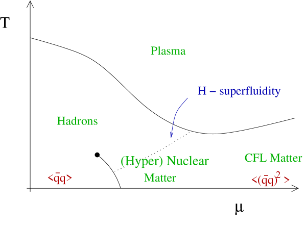
Figure 9: Conjectured phase diagram of $N_{f}=3$ hadronic matter in the limit of exact flavor symmetry.

VIII.2 QCD with three flavors: Color-Flavor-Locking

If quark matter is formed at densities several times nuclear matter density we expect the quark chemical potential to be larger than the strange quark mass. We therefore have to determine the structure of the superfluid order parameter for three quark flavors. We begin with the idealized situation of three degenerate flavors. From the arguments given in the last section we expect the order parameter to be color and flavor anti-symmetric matrix of the form

$$\Phi^{ab}_{ij}=\langle\psi^{a}_{i}C\gamma_{5}\psi^{b}_{j}\rangle.$$ (88)

In order to determine the precise structure of this matrix we have to extremize grand canonical potential. We find Schafer:1999fe ; Evans:1999at

$$\Delta^{ab}_{ij}=\Delta_{A}(\delta_{i}^{a}\delta_{j}^{b}-\delta_{i}^{b}\delta_{j}^{a})+\Delta_{S}(\delta_{i}^{a}\delta_{j}^{b}+\delta_{i}^{b}\delta_{j}^{a}),$$ (89)

which describes the color-flavor locked (CFL) phase proposed in Alford:1999mk . In the weak coupling limit $\Delta_{S}\ll\Delta_{A}$ and $\Delta_{A}=2^{-1/3}\Delta_{0}$ where $\Delta_{0}$ is the gap in the 2SC phase, equ. (86) Schafer:1999fe . In the CFL phase both color and flavor symmetry are completely broken. There are eight combinations of color and flavor symmetries that generate unbroken global symmetries. The unbroken symmetries are

$$\psi^{a}_{L,i}\to(U^{*})^{ab}U_{ij}\psi^{b}_{Lj},\hskip 28.45274pt\psi^{a}_{R,i}\to(U^{*})^{ab}U_{ij}\psi^{b}_{Rj},$$ (90)

for $U\in SU(3)_{V}$. The symmetry breaking pattern is

$$SU(3)_{L}\times SU(3)_{R}\times U(1)_{V}\to SU(3)_{V}.$$ (91)

We observe that color-flavor-locking implies that chiral symmetry is broken. The mechanism for chiral symmetry breaking is quite unusual. The primary order parameter $\langle\psi^{a}_{Li}C\Delta^{ab}_{ij}\psi^{b}_{Lj}\rangle=-\langle\psi^{a}_{Ri}C\Delta^{ab}_{ij}\psi^{b}_{Rj}\rangle$ involves no coupling between left and right handed fermions. In the CFL phase both left and right handed flavor are locked to color, and because of the vectorial coupling of the gluon left handed flavor is effectively locked to right handed flavor. Chiral symmetry breaking also implies that $\langle\bar{\psi}\psi\rangle$ has a non-zero expectation value. We shall compute the quark condensate in Sect. IX.5. In the CFL phase $\langle\bar{\psi}\psi\rangle^{2}\ll\langle(\bar{\psi}\psi)^{2}\rangle$. Another measure of chiral symmetry breaking is provided by the pion decay constant. In Sect. IX.4 we will show that in the weak coupling limit $f_{\pi}^{2}$ is proportional to the density of states on the Fermi surface.

The symmetry breaking pattern $SU(3)_{L}\times SU(3)_{R}\to SU(3)_{V}$ in the CFL phase is identical to the symmetry breaking pattern in QCD at low density. The spectrum of excitations in the color-flavor-locked (CFL) phase also looks remarkably like the spectrum of QCD at low density Schafer:1999ef . The excitations can be classified according to their quantum numbers under the unbroken $SU(3)$, and by their electric charge. The modified charge operator that generates a true symmetry of the CFL phase is given by a linear combination of the original charge operator $Q_{em}$ and the color hypercharge operator $Q={\rm diag}(-2/3,-2/3,1/3)$. Also, baryon number is only broken modulo 2/3, which means that one can still distinguish baryons from mesons. We find that the CFL phase contains an octet of Goldstone bosons associated with chiral symmetry breaking, an octet of vector mesons, an octet and a singlet of baryons, and a singlet Goldstone boson related to superfluidity. All of these states have integer charges.

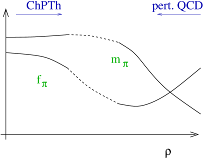
Figure 10: Schematic plot of the properties of hadronic modes in $N_{f}=3$ QCD in the limit of exact flavor symmetries. Hadronic parameters can be determined using chiral perturbation theory at low density, and using perturbative QCD at high density. The high density behavior is studied in Sect. IX.4.

With the exception of the $U(1)$ Goldstone boson, these states exactly match the quantum numbers of the lowest lying multiplets in QCD at low density. In addition to that, the presence of the $U(1)$ Goldstone boson can also be understood. The $U(1)$ order parameter is $\langle(uds)(uds)\rangle$. This order parameter has the quantum numbers of a $0^{+}$ $\Lambda\Lambda$ pair condensate. In $N_{f}=3$ QCD, this is the most symmetric two nucleon channel, and a very likely candidate for superfluidity in nuclear matter at low to moderate density. We conclude that in QCD with three degenerate light flavors, there is no fundamental difference between the high and low density phases. This implies that a low density hyper-nuclear phase and the high density quark phase might be continuously connected, without an intervening phase transition. A conjectured phase diagram is shown in Fig. 9.

An important consistency check for the structure of the phase diagram is provided by anomaly matching arguments. Anomaly matching expresses the requirement that the flavor anomalies of the microscopic theory can be represented in the effective theory for the low energy degrees of freedom tHooft:1980 ; Peskin:1982 . It was shown in Sannino:2000kg ; Sannino:2003pq that this requirement also applies to gauge theories at finite baryon density. We observe that color-flavor-locking realizes the standard Goldstone boson option for anomaly matching in $N_{f}=3$ QCD, whereas the 2SC phase corresponds to the massless proton and neutron option in $N_{f}=2$ QCD.

We also note that the CFL phase provides a weak coupling realization of a phase with chiral symmetry breaking and a mass gap. This means that the CFL phase offers the opportunity to study many of the ’hard’ problems of non-perturbative QCD in a perturbative setting. For example, we can compute hadronic parameters at high baryon density and try to extrapolate the results to low density, see Fig. 10.

VIII.3 $N_{f}\neq 2,3$

Color-flavor locking can be generalized to QCD with more than three flavors Schafer:1999fe . For all $N_{f}\geq 3$ the high density phase is fully gapped. Also, at least part of the chiral $SU(N_{f})\times SU(N_{f})$ symmetry is broken for all $N_{f}\geq 3$, but only in the case $N_{f}=3$ do we find the $T=\mu=0$ pattern of chiral symmetry breaking, $SU(N_{f})_{L}\times SU(N_{f})_{R}\to SU(N_{f})_{V}$.

While the case $N_{f}>3$ is mostly of academic interest, the phase structure of $N_{f}=1$ QCD is possibly relevant to real QCD. Because of mass effects or non-zero electron chemical potentials the Fermi surface of strange and non-strange quarks may get pushed too far apart for strange-non-strange pairing to occur, see Sect. IX.1. As a consequence, there may be regions in the phase diagram where $(ss)$ pairing occurs. In the case of single flavor pairing the order parameter is flavor-symmetric and the Cooper pairs carry non-zero angular momentum. The simplest order parameters are of the form

$$\vec{\Phi}_{1}^{a}=\langle\epsilon^{abc}\psi^{b}C\vec{\gamma}\psi^{c}\rangle,\hskip 28.45274pt\vec{\Phi}_{2}^{a}=\langle\epsilon^{abc}\psi^{b}C\hat{q}\psi^{c}\rangle.$$ (92)

The corresponding gaps can be determined using the methods introduced in section VIII.1. We find $\Delta(\Phi_{1,2})=\exp(-3c_{1,2})\Delta_{0}$ where $c_{1}=-1.5$, $c_{2}=-2$ and $\Delta_{0}$ is the spin zero gap Brown:1999yd ; Schafer:2000tw . While the natural scale of the s-wave gap is $\Delta_{0}\simeq 100$ MeV, the p-wave gap is expected to be less than 1 MeV.

The spin one order parameter equ. (92) is a color-spin matrix. This opens the possibility that color and spin degrees become entangled, similar to the color-flavor-locked phase or the B-phase of liquid ³He. The corresponding order parameter is

$$\Phi_{CSL}=\delta^{a}_{i}\langle\epsilon^{abc}\psi^{b}C\left(\cos(\beta)\hat{q}_{i}+\sin(\beta)\gamma_{i}\right)\psi^{c}\rangle,$$ (93)

where the angle $\beta$ determines the mixing between the two types of condensates shown in equ. (92). A weak coupling analysis of the effective potential shows that the color-spin-locked phase equ. (93) is favored over the “polar” phase equ. (92) Schafer:2000tw . The value of $\beta$ depends sensitively on the interaction and the mass of the quark. In the color-spin-locked phase color and rotational invariance are broken, but a diagonal $SO(3)$ survives. As a consequence, the gap is isotropic. Color-spin-locking also leads to an unusual spectrum of quasi-particles. In the Fermi liquid phase there is a left and right handed color triplet of quarks. In the CSL phase we find a spin 3/2 quartet and a spin 1/2 doublet of the unbroken $SO(3)$ symmetry. The CSL phase ’knows’ that one-flavor nuclear matter consists of spin 3/2 delta baryons.

VIII.4 $N_{c}=2$

QCD with $N_{c}=2$ colors is an interesting model system. The interest in this theory derives from the fact that the determinant of the euclidean Dirac operator in QCD with $N_{c}=2$ remains real even if the baryon chemical potential is non-zero. This means that two-color QCD with an even number of flavors can be studied on the lattice using standard techniques. In addition to that, there is theoretical control not only in the regime of large density, but also in the regime of small density.

For simplicity we will concentrate on the case of $N_{f}=2$ flavors. $SU(2)$ gauge theory has a meson spectrum which is very similar to three-color QCD. Baryons, on the other hand, are bosons rather than fermions and their spectrum is very different as compared to $N_{c}=3$ QCD. Two-color QCD is also characterized by an enlarged chiral symmetry. We can write

$$\Psi=\left(\begin{array}[]{c}\psi_{L}\\ \sigma_{2}\tau_{2}\psi_{R}^{*}\end{array}\right),$$ (94)

where $\sigma_{2},\tau_{2}$ are anti-symmetric color and flavor $SU(2)$ matrices. Two-color QCD is not only invariant under $SU(2)_{L}\times SU(2)_{R}$ transformations acting on the upper and lower components of $\Psi$ separately, but under the full $SU(4)$ group Peskin:1980gc ; Rapp:1998zu ; Kogut:1999iv . The $SU(4)$ chiral symmetry mixes the quark-anti-quark condensate $\langle\bar{\psi}^{a}\psi^{a}\rangle$ with the diquark condensate $\langle\epsilon^{ab}\psi^{a\,T}C\gamma_{5}\tau_{2}\psi^{b}\rangle$.

At zero temperature and density, and in the presence of a small quark mass, the chiral $SU(4)$ symmetry is broken to $Sp(4)$ by a quark-anti-quark condensate $\langle\bar{\psi}^{a}\psi^{a}\rangle$. There are 5 Goldstone bosons, three pions $\vec{\pi}$, the scalar diquark $S$ and the scalar anti-diquark $\bar{S}$. If we turn on a baryon chemical potential then the scalar diquark will Bose condense if the chemical potential exceeds the mass of the diquark. Since the scalar diquark is a Goldstone boson, this phenomenon can be studied using the chiral effective lagrangian of $N_{c}=2$ QCD. The effective lagrangian is given by Kogut:1999iv ; Kogut:2000ek

$${\cal L}=\frac{f_{\pi}^{2}}{4}{\rm Tr}\left[D_{\mu}\Sigma D^{\mu}\Sigma^{\dagger}\right]+\Big{[}mC{\rm Tr}(\hat{M}\Sigma^{\dagger})+h.c.\Big{]}+\ldots.$$ (95)

The chiral field $\Sigma$ parametrizes the coset $SU(4)/Sp(4)$. $\Sigma$ is an anti-symmetric unitary matrix. It transforms as $\Sigma\to U\Sigma U^{T}$ under the chiral $SU(4)$ symmetry. The covariant derivative is defined as

$$iD_{\nu}=i\partial_{\nu}-\mu\delta_{\nu 0}\left(\hat{B}\Sigma+\Sigma\hat{B}^{T}\right).$$ (96)

The matrices $\hat{M}$ and $\hat{B}$ are determined by the transformation properties of the mass term $m\bar{\psi}\psi$ and the chemical potential term $\mu\psi^{\dagger}\psi$ under the chiral $SU(4)$ symmetry. We have

$$\hat{M}=\left(\begin{array}[]{cc}0&1\\ -1&0\end{array}\right),\hskip 28.45274pt\hat{B}=\left(\begin{array}[]{cc}1&0\\ 0&-1\end{array}\right).$$ (97)

We can determine the ground state by minimizing the potential

$$V(\Sigma)=-\frac{f_{\pi}^{2}}{2}{\rm Tr}\left[\Sigma B^{T}\Sigma^{\dagger}B\right]+\Big{[}mC{\rm Tr}(\hat{M}\Sigma^{\dagger})+h.c.\Big{]}.$$ (98)

For zero density and finite quark mass the minimum is $\Sigma_{\bar{q}q}=\hat{M}$. In this state $SU(4)$ is broken to $Sp(4)$. Goldstone bosons are described by fluctuations $\Sigma=U\Sigma_{\bar{q}q}U^{T}$ with $U=\exp(i\phi^{a}X^{a}/f_{\pi})\in SU(4)/Sp(4)$. Here, $X^{a}$ are the $SU(4)$ generators that act non-trivially on $\Sigma_{\bar{q}q}$. As mentioned above, there a 5 Goldstone modes.

The first term in equ. (98) is minimized by

$$\Sigma_{qq}=\left(\begin{array}[]{cc}\sigma_{2}&0\\ 0&\sigma_{2}\end{array}\right).$$ (99)

For non-zero chemical we expect the minimum to be of the form $\Sigma_{0}=\Sigma_{\bar{q}q}\cos(\alpha)+\Sigma_{qq}\sin(\alpha)$. Substituting this ansatz into equ. (98) we find $\alpha=0$ for $\mu<m_{\pi}/2$ and $\cos(\alpha)=m_{\pi}^{2}/(4\mu)^{2}$. Differentiating the effective potential with respect to the chemical potential we find the baryon density

$$\rho_{B}=8f_{\pi}^{2}\mu\left(1-\left(\frac{m_{\pi}^{2}}{4\mu^{2}}\right)^{2}\right).$$ (100)

For small $\mu=m_{\pi}/2+\delta\mu$ this result is exactly of the same form as equ. (26). This implies that the physical phenomenon is indeed Bose condensation of scalar diquarks interacting through a short range repulsive interaction.

If the density becomes large, $\mu\sim m_{\rho}\gg m_{\pi}$, the effective lagrangian description breaks down. On the other hand, if $\mu\gg\Lambda_{QCD}$ we expect to find a perturbative BCS superfluid of diquark pairs. The gap and the superfluid condensate can be computed using the methods discussed in Sect. VIII.1. We find

$$\Delta=512\pi^{4}b_{0}^{\prime}\mu g^{-5}\exp\left(-\frac{2\pi^{2}}{g}\right),$$ (101)

with $b_{0}^{\prime}=\exp(-(\pi^{2}+4)/16)$. Numerical studies on the lattice can be used in order to verify the limiting behavior at small and large density, and to study the Bose condensation/BCS crossover, see Kogut:2002cm and references therein. Similar studies have also been performed in the instanton liquid model Schafer:1998up . There are many other interesting questions that can be studied in two-color QCD. It was suggested, for example, that vector mesons (diquarks) may condense if the chemical potential is on the order of the vector meson mass Lenaghan:2001sd ; Sannino:2002wp . Other interesting questions concern the structure of the phase diagram at non-zero temperature Splittorff:2002xn , and the nature of the deconfinement transition. It was also pointed out that the behavior of the $\eta^{\prime}$ mass in two-color QCD can be used in order to study the mechanism of $U(1)_{A}$ breaking in QCD Schafer:2002yy . Finally, we should mention that there are some other gauge theories in which the euclidean fermion determinant is positive even if the chemical potential is non-zero. These theories include QCD at finite isospin chemical potential and QCD with a non-zero density of quarks in the adjoint representation of color Alford:1998sd ; Son:2000xc ; Kogut:2000ek . It is amusing that all of these theories have Goldstone bosons that carry the conserved charge. As a consequence, the low density state of these theories is a dilute Goldstone boson condensate, similar to the $N_{c}=2$ diquark condensate studied in this section.

VIII.5 $N_{c}\to\infty$

In the large $N_{c}$ limit quark-quark scattering is suppressed as compared to quark-quark-hole scattering. The color factors in the two channels are

$$c=\frac{N_{c}+1}{2N_{c}}\hskip 14.22636pt(qq),\hskip 28.45274ptc=\frac{N_{c}^{2}-1}{2N_{c}}\hskip 14.22636pt(qh),$$ (102)

suggesting that particle-particle pairing, and superconductivity, is disfavored at large $N_{c}$. As a consequence, other forms of pairing may take place. Particle-hole scattering is not suppressed, but particle-hole pairing can only take place over a small part of the Fermi surface. The order parameter for particle-hole pairing is Deryagin:1992

$$\langle\bar{\psi}(x)\psi(y)\rangle=\exp(i\vec{p}\cdot(\vec{x}+\vec{y}))\Sigma(x-y),$$ (103)

where $|\vec{p}|=p_{F}$ is a vector on the Fermi surface. This state describes a chiral density wave. It resembles a charge or spin density wave in quasi-one-dimensional condensed matter systems Gruner . QCD, of course, is not quasi-one-dimensional but at large $N_{c}$ screening due to fermions is weak and the perturbative one-gluon exchange interaction is very strongly dominated by collinear scattering. The problem was studied in the weak coupling approximation in Shuster:1999 . It was found that the transition from color superconductivity to chiral density waves requires very large values of $N_{c}>1000$. On the other hand, if the coupling is strong and the density is not too large, then the chiral density wave state may compete with color superconductivity even for three colors Rapp:2000zd .

IX The role of the strange quark mass

IX.1 BCS theory: toy model

At baryon densities relevant to astrophysical objects distortions of the pure CFL state due to non-zero quark masses cannot be neglected Alford:1999pa ; Schafer:1999pb ; Rapp:1999qa ; Bedaque:1999nu ; Alford:2000ze ; Schafer:2000ew ; Bedaque:2001je ; Kaplan:2001qk ; Casalbuoni:2002st ; Fugleberg:2002rk ; Casalbuoni:2003cs . The most important effect of a non-zero strange quark mass is that the light and strange Fermi surfaces will no longer be of equal size. When the mismatch is much smaller than the gap one calculates assuming degenerate quarks, we might expect that it has very little consequence, since at this level the original particle and hole states near the Fermi surface are mixed up anyway. On the other hand, when the mismatch is much larger than the nominal gap, we might expect that the ordering one would obtain for degenerate quarks is disrupted, and that to a first approximation one can treat the light and heavy quark dynamics separately.

Figure 11: Light quark gap $\Delta_{ud}$ and strange-non-strange gap $\Delta_{us}$ as a function of the strange quark mass for $\mu=0.5$ GeV. This figure shows the result of a mean field analysis based on a schematic BCS interaction Schafer:1999pb . The interaction strength was (arbitrarily) adjusted to $\Delta_{ud}(m_{s}\!=\!0)=25$ MeV.

We can see this in a more quantitative fashion by studying a schematic gap equation that describes the spin singlet pairing of two fermions with different masses. In a basis of particles of the first kind and holes of the second the quadratic part of the action is

$${\cal S}=\int\frac{d^{4}p}{(2\pi)^{4}}\left(\psi^{\dagger}_{(1)}\hskip 8.5359pt\psi_{(2)}\right)\left(\begin{array}[]{cc}p_{0}-\epsilon_{p}^{1}&\Delta\\ \Delta^{*}&p_{0}+\epsilon_{p}^{2}\end{array}\right)\left(\begin{array}[]{c}\psi_{(1)}\\ \psi^{\dagger}_{(2)}\end{array}\right).$$ (104)

Here, $\epsilon^{1,2}_{p}=E^{1,2}_{p}-\mu$ and $E^{1,2}_{p}=(p^{2}+m_{1,2}^{2})^{1/2}$ where $m_{1,2}$ are the masses of particle one and two. The particle and hole propagators are determined by the inverse of the matrix equ. (104). The off-diagonal (anomalous) propagator is

$$G_{21}=\frac{\Delta}{(p_{0}-\epsilon^{1}_{p})(p_{0}+\epsilon^{2}_{p})-\Delta^{2}}.$$ (105)

We study the effect of a zero range interaction $G(\psi_{1}\sigma_{2}\psi_{2})(\psi^{\dagger}_{1}\sigma_{2}\psi^{\dagger}_{2})$. The pairing is described by the gap equation

$$\Delta=G\int\frac{d^{4}p}{(2\pi)^{4}}\frac{\Delta}{(p_{0}+R+i\delta{\rm sgn}(p_{0}))^{2}-\bar{\epsilon}_{p}^{2}-\Delta^{2}}.$$ (106)

Here, we have introduced $\bar{\epsilon}_{p}=\bar{E}_{p}-\mu=(\epsilon^{1}_{p}+\epsilon^{2}_{p})/2$ and $R=(\epsilon^{1}_{p}-\epsilon^{2}_{p})/2$. In practice, we are interested in pairing between almost massless up or down quarks and massive strange quarks. In that case, $R\simeq m_{s}^{2}/(4p_{F})\simeq m_{s}^{2}/(4\mu)$. The poles of the anomalous propagator are located at $p_{0}=-R\pm(\bar{\epsilon}^{2}_{p}+\Delta^{2})^{1/2}-i{\rm sgn}(p_{0})$. As usual, we close the integration contour in the lower half plane. Let us denote the solution of the gap equation in the case $R=0$ by $\Delta_{0}$. Then, if $R<\Delta_{0}$, the pole with the positive sign of the square root is always included in the integration contour and we have

$$\Delta=\frac{G\mu^{2}}{4\pi^{2}}\int d\bar{\epsilon}_{p}\,\frac{\Delta}{\sqrt{\bar{\epsilon}^{2}_{p}+\Delta^{2}}}.$$ (107)

This result is, up to a small correction in the density of states that we have neglected here, identical to the gap equation for degenerate fermions, so $\Delta\approx\Delta_{0}$. If, on the other hand, $R>\Delta_{0}$ there only is a pole in the lower half plane if $\bar{\epsilon}_{p}>\sqrt{R^{2}-\Delta^{2}}$. Carrying out the $p_{0}$ integration again leads to the gap equation (107), but with the $\bar{\epsilon}_{p}$ integration restricted by the condition just mentioned. This cuts out the infrared singularity at $\bar{\epsilon}_{p}=0$ and one can easily verify that the gap equation does not have a non-trivial solution for weak coupling. We thus conclude that a necessary condition for pairing is that

$$m_{s}^{2}<m_{s}^{2}({\it crit})\simeq 4p_{F}\Delta(m_{s}\!=\!0).$$ (108)

IX.2 BCS theory: CFL phase

So far, we have only dealt with a simple pair condensate involving strange and non-strange quarks. In practice, we are interested in a somewhat more complicated situation. In particular, we want to consider the transition between the color-flavor locked phase for small $m_{s}$ and the two-flavor color superconductor in the limit of large $m_{s}$. This analysis can be carried out along the same lines as the toy model discussed above. We now consider the following free action Schafer:1999pb ; Alford:1999pa

$$S=\int\frac{d^{4}p}{(2\pi)^{4}}\left(\psi^{\dagger}\hskip 8.5359pt\psi\right)\left(\begin{array}[]{cc}(p_{0}-\epsilon_{p})X_{1}-2RX_{s}&\Delta_{ud}X_{ud}+\Delta_{us}X_{us}\\ \Delta_{ud}X_{ud}+\Delta_{us}X_{us}&(p_{0}+\epsilon_{p})X_{1}+2RX_{s}\end{array}\right)\left(\begin{array}[]{c}\psi\\ \psi^{\dagger}\end{array}\right),$$ (109)

where $\psi$ is now a 9 component color-flavor spinor. $X_{1},X_{s},X_{ud}$ and $X_{us}$ are color-flavor matrices

$$\begin{array}[]{rclrcl}X_{1}&=&\delta^{\alpha\beta}\delta_{ab},&X_{s}&=&\delta^{\alpha\beta}\delta_{a3}\delta_{b3}\\ X_{ud}&=&\epsilon^{3\alpha\beta}\epsilon_{3ab},&X_{us}&=&\epsilon^{2\alpha\beta}\epsilon_{2ab}+\epsilon^{1\alpha\beta}\epsilon_{1ab},\end{array}$$ (110)

where $\alpha,\beta$ are color, and $a,b$ flavor indices. $\Delta_{ud}$ is the gap for $\langle ud\rangle$ condensation, and $\Delta_{us}$ is the gap for $\langle us\rangle=\langle ds\rangle$ condensation. Color-flavor locking corresponds to the case $\Delta_{ud}=\Delta_{us}$, and the two flavor superconductor corresponds to $\Delta_{us}=0,\,\Delta_{ud}\neq 0$.

Flavor symmetry breaking is again caused by $R\simeq m_{s}^{2}/(4p_{F})$. The Nambu-Gorkov matrix equ. (109) can be diagonalized exactly. The eigenvalues and their degeneracies are

$$\begin{array}[]{ll}p_{0}\pm\left(\epsilon_{p}^{2}+\Delta_{ud}^{2}\right)^{1/2},&d=3\\ p_{0}-R\pm\left(\bar{\epsilon}_{p}^{2}+\Delta_{us}^{2}\right)^{1/2},&d=2\\ p_{0}+R\pm\left(\bar{\epsilon}_{p}^{2}+\Delta_{us}^{2}\right)^{1/2},&d=2\\ p_{0}\pm\left(\epsilon_{p}^{2}+2R\epsilon_{p}+2R^{2}+2\Delta_{us}^{2}+\frac{1}{2}\Delta_{ud}^{2}\pm\frac{1}{2}S\right)^{1/2},&d=1,1\\ \end{array}$$ (111)

where

$$S=\left(8\Delta_{us}^{2}\left(\Delta_{ud}^{2}+4R^{2}\right)+\left(\Delta_{ud}^{2}-4R(\epsilon_{p}+R)\right)^{2}\right)^{1/2}.$$ (112)

The result becomes easier to understand if we consider some simple limits. If we ignore flavor symmetry breaking, $R=0$, and set $\Delta_{ud}=\Delta_{us}$ we find 8 eigenvalues $p_{0}\pm(\epsilon_{p}^{2}+\Delta^{2})^{1/2}$ and one eigenvalue with the gap $2\Delta$. These states fill out an octet and a singlet of the unbroken $SU(3)_{F}$ symmetry of the CFL phase. If, on the other hand, we set $\Delta_{us}=0$ we find 4 eigenvalues $p_{0}\pm(\epsilon_{p}^{2}+\Delta^{2})^{1/2}$ while the other 5 eigenvalues have vanishing gaps. This is the spectrum of the $N_{f}=2$ phase. If flavor symmetry is broken, we find that the $SU(3)$ octet splits into two $SU(2)$ doublets, one triplet and singlet.

We note that in the presence of flavor symmetry breaking the first three eigenvalues, which depend on $\Delta_{ud}$ only, are completely unaffected. For the next 4 eigenvalues, which only depend on $\Delta_{us}$, the energy $p_{0}$ is effectively shifted by $R$. This is exactly as in the simple toy model discussed above. It implies that for $R>\Delta_{us}$, when we close the integration contour in the complex $p_{0}$ plane, we do not pick up this pole. The last two eigenvalues are more complicated. They depend on both $\Delta_{ud}$ and $\Delta_{us}$, and they explicitly contain the flavor symmetry breaking parameter $R$. Nevertheless, the structure of the eigenvalues is certainly suggestive of the idea that for $R<\Delta_{us}^{0}$ we have $\Delta_{us}\simeq\Delta_{ud}$, and the gaps are almost independent of $R$, while at $R\simeq\Delta_{us}^{0}$ there is a discontinuity and $\Delta_{us}$ goes to zero.

This is borne out by a more detailed calculation. For this purpose, we add a flavor and color anti-symmetric short range interaction

$${\cal L}=\frac{K}{4}\big{(}\delta^{\alpha\gamma}\delta^{\beta\delta}-\delta^{\alpha\delta}\delta^{\beta\gamma}\big{)}\big{(}\delta_{ac}\delta_{bd}-\delta_{ad}\delta_{bc}\big{)}\,\left(\psi^{\alpha}_{a}\sigma_{2}\psi^{\beta}_{b}\right)\left(\psi^{\gamma\,\dagger}_{c}\sigma_{2}\psi^{\delta\,\dagger}_{d}\right).$$ (113)

The free energy of the system is the sum of the quasi-particle contribution equ. (111) and the mean field potential $V=1/K\cdot(\Delta_{ud}^{2}+2\Delta_{us}^{2})$. There are two coupled gap equations, which can be derived by varying the free energy with respect to the two parameters $\Delta_{ud}$ and $\Delta_{us}$. A typical numerical result is shown in Fig. 11. We observe that the flavor symmetry breaking difference $\Delta_{ud}-\Delta_{us}$ is quite small all the way up to the critical strange quark mass. At the critical mass, there is a discontinuous transition to a phase where $\Delta_{us}$ vanishes exactly. The value of the critical mass is very close to the estimate $m_{s}=2\sqrt{\mu\Delta_{us}^{0}}$.

A number of authors have improved on the treatment presented in this section, in particular by studying the consequences of imposing electric and color charge neutrality Steiner:2002gx ; Alford:2002kj ; Neumann:2002jm . In the BCS framework one finds that once charge neutrality is imposed the number density of up, down and strange quarks in the CFL phase is exactly the same, even in the presence of flavor symmetry breaking. As a consequence, the CFL phase does not require the presence of electrons to be electrically neutral Rajagopal:2000ff .

Another interesting question concerns the possibility of additional phases that interpolate between the CFL and $N_{f}=2$ (2SC) superfluids. In Shovkovy:2003uu ; Gubankova:2003uj it was shown that the charge neutrality constraint may help to stabilize gapless (‘breached’) CFL phases for $m_{s}>m_{s}({\it crit})$. Also, if the mismatch between the strange and non-strange Fermi surfaces is too large for BCS pairing to occur, pairing may still take place with a spatially varying superfluid order parameter Alford:2000ze . This phase is known as the LOFF (Larkin-Ovchinikov-Fulde-Ferell) phase Larkin:1964 ; Fulde:1964 ; Abrikosov:1988 . The LOFF phase is distinguished by an interesting crystal structure Bowers:2002xr .

All of these studies are based on an ansatz for the structure of the CFL phase in the presence of flavor symmetry breaking. This is somewhat unsatisfactory. In weak coupling and in the limit $m_{s}\ll m_{s}({\it crit})$ we should be able to perform rigorous calculations. Also, in the BCS approximation we find that the quark densities in the CFL phase remain exactly equal even if the strange quark mass or the electron chemical potential are non-zero. However, the CFL phase contains almost massless flavored Goldstone bosons, so the response to any external perturbation that can couple to Goldstone modes should not vanish.

In the following section we will show how to study the effect of a non-zero strange mass using an effective field theory of the CFL phase Casalbuoni:1999wu . This theory determines both the ground state and the spectrum of excitations with energies below the gap in the CFL phase. Using the effective theory allows us to perform systematic calculations order by order in the quark mass.

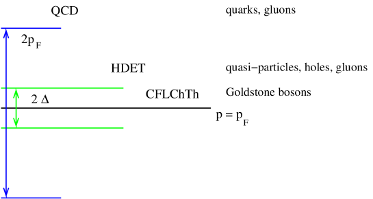
Figure 12: Hierarchy of effective field theories in the CFL phase.

IX.3 CFL chiral theory

For excitation energies smaller than the gap the only relevant degrees of freedom are the Goldstone modes associated with the breaking of chiral symmetry and baryon number, see Fig. 12. The interaction of the Goldstone modes is described by an effective lagrangian of the form Casalbuoni:1999wu

$${\cal L}_{eff} = \frac{f_{\pi}^{2}}{4}{\rm Tr}\left[\nabla_{0}\Sigma\nabla_{0}\Sigma^{\dagger}-v_{\pi}^{2}\partial_{i}\Sigma\partial_{i}\Sigma^{\dagger}\right]+\Big{[}B{\rm Tr}(M\Sigma^{\dagger})+h.c.\Big{]}$$

$$\mbox{}+\Big{[}A_{1}{\rm Tr}(M\Sigma^{\dagger}){\rm Tr}(M\Sigma^{\dagger})+A_{2}{\rm Tr}(M\Sigma^{\dagger}M\Sigma^{\dagger})+A_{3}{\rm Tr}(M\Sigma^{\dagger}){\rm Tr}(M^{\dagger}\Sigma)+h.c.\Big{]}+\ldots.$$

Here $\Sigma=\exp(i\phi^{a}\lambda^{a}/f_{\pi})$ is the chiral field, $f_{\pi}$ is the pion decay constant and $M$ is a complex mass matrix. The chiral field and the mass matrix transform as $\Sigma\to L\Sigma R^{\dagger}$ and $M\to LMR^{\dagger}$ under chiral transformations $(L,R)\in SU(3)_{L}\times SU(3)_{R}$. We have suppressed the singlet fields associated with the breaking of the exact $U(1)_{V}$ and approximate $U(1)_{A}$ symmetries. As with ordinary chiral perturbation theory, the structure of the effective lagrangian is entirely determined by the symmetries. At low density the coefficients $f_{\pi}$, $B,A_{i},\ldots$ are non-perturbative quantities that have to extracted from experiment or measured on the lattice. At large density, on the other hand, the chiral coefficients can be calculated in perturbative QCD.

Superficially, equ. (IX.3) looks exactly like ordinary chiral perturbation theory. There are, however, some important differences. Lorentz invariance is broken and Goldstone modes move with the velocity $v_{\pi}<c$. The chiral expansion has the structure

$${\cal L}\sim f_{\pi}^{2}\Delta^{2}\left(\frac{\partial_{0}}{\Delta}\right)^{k}\left(\frac{\vec{\partial}}{\Delta}\right)^{l}\big{(}\Sigma\big{)}^{m}\big{(}\Sigma^{\dagger}\big{)}^{n}.$$ (115)

Loop graphs are suppressed by powers of $p/(4\pi f_{\pi})$. We shall see that the pion decay constant scales as $f_{\pi}\sim p_{F}$. As a result loops are suppressed by $p/p_{F}$ whereas higher order contact terms are suppressed by $p/\Delta$. This means that in the CFL chiral theory pion loops with leading order vertices are parametrically small as compared to higher order contact terms, whereas in ordinary chiral perturbation theory the two are comparable in size.

Further differences as compared to chiral perturbation theory in vacuum appear when the expansion in the quark mass is considered. The CFL phase has an approximate $(Z_{2})_{A}$ symmetry under which $M\to-M$ and $\Sigma\to\Sigma$. This symmetry implies that the coefficients of mass terms that contain odd powers of $M$ are small. The $(Z_{2})_{A}$ symmetry is explicitly broken by instantons. The coefficient $B$ can be determined from a weak coupling instanton calculation and $B\sim(\Lambda_{QCD}/p_{F})^{8}$, see Sect. IX.5.

A priori it is also not clear what the expansion parameter in the chiral expansion is. There are several dimensionless ratios that can appear, $(m/p_{F}),(m/\Delta)$ and $(m/\Lambda_{QCD})$. The BCS calculations discussed in the previous section suggest that the CFL phase undergoes a phase transition to a less symmetric phase when $m^{2}/(2p_{F})\sim\Delta$. This result indicates that the expansion parameter is $M^{2}/(p_{F}\Delta)$. We shall see that this is indeed the case. However, the coefficients $A_{i}$ of the quadratic terms in $M$ turn out to be anomalously small. In Sect. IX.4 we will show that

$$A_{i}M^{2}\sim\Delta^{2}M^{2}\sim f_{\pi}^{2}\Delta^{2}\left(\frac{M^{2}}{p_{F}^{2}}\right),$$ (116)

compared to the naive estimate $A_{i}M^{2}\sim f_{\pi}^{2}\Delta^{2}[M^{2}/(p_{F}\Delta)]$.

The pion decay constant $f_{\pi}$ and the coefficients $A_{i}$ can be determined using matching techniques. Matching expresses the requirement that Green functions in the effective chiral theory and the underlying microscopic theory, QCD, agree. The pion decay constant is most easily determined by coupling $SU(N_{f})_{L,R}$ gauge fields $W_{L,R}$ to the left and right flavor currents. As usual, this amounts to replacing ordinary derivatives by covariant derivatives. The time component of the covariant derivative is given by $\nabla_{0}\Sigma=\partial_{0}\Sigma+iW_{L}\Sigma-i\Sigma W_{R}$ where we have suppressed the vector index of the gauge fields. In the CFL vacuum $\Sigma=1$ the axial gauge field $W_{L}-W_{R}$ acquires a mass by the Higgs mechanism. From equ. (IX.3) we get

$${\cal L}=\frac{f_{\pi}^{2}}{4}\,\frac{1}{2}(W_{L}-W_{R})^{2}.$$ (117)

The coefficients $B$ and $A_{1,2,3}$ can be determined by computing the shift in the vacuum energy due to non-zero quark masses in both the chiral theory and the microscopic theory. In the chiral theory we have

$$\Delta{\cal E}=-\Big{[}B{\rm Tr}(M)+A_{1}\left({\rm Tr}(M)\right)^{2}+A_{2}{\rm Tr}(M^{2})+A_{3}{\rm Tr}(M){\rm Tr}(M^{\dagger})+h.c.\Big{]}.$$ (118)

We note that as long as we keep track of the difference between $M$ and $M^{\dagger}$ different $O(M^{2})$ mass terms produce distinct contributions to the vacuum energy. This means that the coefficients $A_{i}$ can be reconstructed uniquely from the vacuum energy.

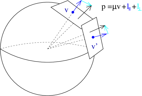
Figure 13: High density effective field theory description of the Fermi surface.

IX.4 High density effective theory

In this section we shall determine the mass of the gauge field and the shift in the vacuum energy in the CFL phase of QCD at large baryon density. This is possible because asymptotic freedom guarantees that the effective coupling is weak. The QCD Lagrangian in the presence of a chemical potential is given by

$${\cal L}=\bar{\psi}\left(iD/\,+\mu\gamma_{0}\right)\psi-\bar{\psi}_{L}M\psi_{R}-\bar{\psi}_{R}M^{\dagger}\psi_{L}-\frac{1}{4}G^{a}_{\mu\nu}G^{a}_{\mu\nu},$$ (119)

where $D_{\mu}=\partial_{\mu}+igA_{\mu}$ is the covariant derivative, $M$ is the mass matrix and $\mu$ is the baryon chemical potential. If the baryon density is very large perturbative QCD calculations can be further simplified. The main observation is that the relevant degrees of freedom are particle and hole excitations in the vicinity of the Fermi surface. We shall describe these excitations in terms of the field $\psi_{+}(\vec{v},x)$, where $\vec{v}$ is the Fermi velocity. The field $\psi_{+}(\vec{v},x)$ is defined on patches that cover the Fermi surface, see Fig. 13. Soft collinear scatterings take place within a given patch whereas hard interactions can scatter Fermions from one patch to another.

At tree level, the quark field $\psi$ can be decomposed as $\psi=\psi_{+}+\psi_{-}$ where $\psi_{\pm}=\frac{1}{2}(1\pm\vec{\alpha}\cdot\hat{v})\psi$. To leading order in $1/p_{F}$ we can eliminate the field $\psi_{-}$ using its equation of motion. For $\psi_{-,L}$ we find

$$\psi_{-,L}=\frac{1}{2p_{F}}\left(i\vec{\alpha}_{\perp}\cdot\vec{D}\psi_{+,L}+\gamma_{0}M\psi_{+,R}\right).$$ (120)

There is a similar equation for $\psi_{-,R}$. The longitudinal and transverse components of $\gamma_{\mu}$ are defined by $(\gamma_{0},\vec{\gamma})_{\|}=(\gamma_{0},\vec{v}(\vec{\gamma}\cdot\vec{v}))$ and $(\gamma_{\mu})_{\perp}=\gamma_{\mu}-(\gamma_{\mu})_{\|}$. To leading order in $1/p_{F}$ the lagrangian for the $\psi_{+}$ field is given by Hong:2000tn ; Hong:2000ru ; Beane:2000ms

$${\cal L} = \psi_{L+}^{\dagger}(iv\cdot D)\psi_{L+}-\frac{\Delta}{2}\left(\psi_{L+}^{ai}C\psi_{L+}^{bj}\left(\delta_{ai}\delta_{bj}-\delta_{aj}\delta_{bi}\right)+{\rm h.c.}\right)$$ (121)

$$\hskip 14.22636pt\mbox{}-\frac{1}{2p_{F}}\psi_{L+}^{\dagger}\left((D/\,_{\perp})^{2}+MM^{\dagger}\right)\psi_{L+}+\left(R\leftrightarrow L,M\leftrightarrow M^{\dagger}\right)+\ldots,$$

with $v_{\mu}=(1,\vec{v})$ and $i,j,\ldots$ and $a,b,\ldots$ denote flavor and color indices. In order to perform perturbative calculations in the superconducting phase we have added a tree level gap term $\psi^{ai}_{L,R}C\Delta_{ai,bj}\psi^{bj}_{L,R}$. In the CFL phase this term has the structure $\Delta_{ai,bj}=\Delta(\delta_{ai}\delta_{bj}-\delta_{aj}\delta_{bi})$. The magnitude of the gap $\Delta$ is determined order by order in perturbation theory from the requirement that the thermodynamic potential is stationary with respect to $\Delta$. With the gap term included the perturbative expansion is well defined.

The screening mass of the flavor gauge fields $W_{L,R}$ can be determined by computing the corresponding polarization function in the limit $q_{0}=0$, $\vec{q}\to 0$. The relevant diagrams are shown in Fig. 14, see Son:1999cm ; Bedaque:2001je . The first two diagrams do not involve mixing between left and right-handed currents. The third diagram involves mixing between left and right handed currents and is unique to the CFL phase. We find

$$\Pi^{LL}_{00}=\Pi^{RR}_{00}=-\Pi^{LR}_{00}=\frac{m_{D}^{2}}{4},\hskip 14.22636ptm_{D}^{2}=\frac{21-8\log(2)}{18}\left(\frac{p_{F}^{2}}{2\pi^{2}}\right).$$ (122)

Matching equ. (122) against equ. (117) we get Son:1999cm ; Zarembo:2000pj ; Miransky:2001bd

$$f_{\pi}^{2}=\frac{21-8\log(2)}{18}\left(\frac{p_{F}^{2}}{2\pi^{2}}\right).$$ (123)

Repeating the matching calculation for the spatial components of the polarization tensor we get $v_{\pi}^{2}=1/3$ Son:1999cm .

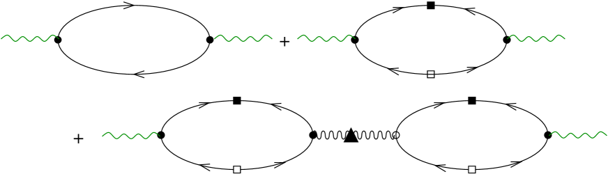
Figure 14: Diagrams in the high density effective theory that contribute to the chiral flavor current polarization function at leading order in $g$. The green wiggly lines are flavor currents, while the black wiggly line is a gluon propagator. Squares are anomalous fermion self energy insertions, and the triangle is a gluon self energy insertion.

Our next task is to compute the mass dependence of the vacuum energy. To leading order in $1/p_{F}$ there is only one operator in the high density effective theory

$${\cal L}=-\frac{1}{2p_{F}}\left(\psi_{L+}^{\dagger}MM^{\dagger}\psi_{L+}+\psi_{R+}^{\dagger}M^{\dagger}M\psi_{R+}\right).$$ (124)

This term arises from expanding the kinetic energy of a massive fermion around $p=p_{F}$. We note that $MM^{\dagger}/(2p_{F})$ and $M^{\dagger}M/(2p_{F})$ act as effective chemical potentials for left and right-handed fermions, respectively. Indeed, to leading order in the $1/p_{F}$ expansion, the Lagrangian equ. (121) is invariant under a time dependent flavor symmetry $\psi_{L}\to L(t)\psi_{L}$, $\psi_{R}\to R(t)\psi_{R}$ where $X_{L}=MM^{\dagger}/(2p_{F})$ and $X_{R}=M^{\dagger}M/(2p_{F})$ transform as left and right-handed flavor gauge fields. If we impose this approximate gauge symmetry on the CFL chiral theory we have to include the effective chemical potentials $X_{L,R}$ in the covariant derivative of the chiral field Bedaque:2001je ,

$$\nabla_{0}\Sigma=\partial_{0}\Sigma+i\left(\frac{MM^{\dagger}}{2p_{F}}\right)\Sigma-i\Sigma\left(\frac{M^{\dagger}M}{2p_{F}}\right).$$ (125)

$X_{L}$ and $X_{R}$ contribute to the vacuum energy at $O(M^{4})$

$$\Delta{\cal E}=\frac{f_{\pi}^{2}}{8p_{F}^{2}}{\rm Tr}\left[(MM^{\dagger})(M^{\dagger}M)-(MM^{\dagger})^{2}\right].$$ (126)

This result can also be derived directly in the microscopic theory Bedaque:2001je . The corresponding diagrams are exactly the same diagrams that appear in the calculation of $f_{\pi}$, Fig. 14, but with the external flavor gauge fields replaced by insertions of equ. (124). We also note that equation (126) has the expected scaling behavior ${\cal E}\sim f_{\pi}^{2}\Delta^{2}[M^{2}/(p_{F}\Delta)]^{2}$.

$O(M^{2})$ terms in the vacuum energy are generated by terms in the high density effective theory that are higher order in the $1/p_{F}$ expansion. These terms can be determined by computing chirality violating quark-quark scattering amplitudes for fermions in the vicinity of the Fermi surface Schafer:2001za . Feynman diagrams for $q_{L}+q_{L}\to q_{R}+q_{R}$ are shown in Fig. 15b. To leading order in the $1/p_{F}$ expansion the chirality violating scattering amplitudes are independent of the scattering angle and can be represented as local four-fermion operators

$${\cal L}=\frac{g^{2}}{8p_{F}^{4}}\left(({\psi^{A}_{L}}^{\dagger}C{\psi^{B}_{L}}^{\dagger})(\psi^{C}_{R}C\psi^{D}_{R})\Gamma^{ABCD}+({\psi^{A}_{L}}^{\dagger}\psi^{B}_{L})({\psi^{C}_{R}}^{\dagger}\psi^{D}_{R})\tilde{\Gamma}^{ACBD}\right).$$ (127)

There are two additional terms with $(L\leftrightarrow R)$ and $(M\leftrightarrow M^{\dagger})$. We have introduced the CFL eigenstates $\psi^{A}$ defined by $\psi^{a}_{i}=\psi^{A}(\lambda^{A})_{ai}/\sqrt{2}$, $A=0,\ldots,8$. The tensor $\Gamma$ is defined by

$$\Gamma^{ABCD} = \frac{1}{8}\Big{\{}{\rm Tr}\left[\lambda^{A}M(\lambda^{D})^{T}\lambda^{B}M(\lambda^{C})^{T}\right]$$ (128)

$$\hskip 28.45274pt\mbox{}-\frac{1}{3}{\rm Tr}\left[\lambda^{A}M(\lambda^{D})^{T}\right]{\rm Tr}\left[\lambda^{B}M(\lambda^{C})^{T}\right]\Big{\}}.$$

The second tensor $\tilde{\Gamma}$ involves both $M$ and $M^{\dagger}$ and only contributes to terms of the form ${\rm Tr}[MM^{\dagger}]$ in the vacuum energy. These terms do not contain the chiral field $\Sigma$ and therefore do not contribute to the masses of Goldstone modes. We can now compute the shift in the vacuum energy due to the effective vertex equ. (127). The leading contribution comes from the two-loop diagram shown in Fig. 15. This diagram is proportional to the square of the superfluid density. We find

$$\Delta{\cal E}=-\frac{3\Delta^{2}}{4\pi^{2}}\left\{\Big{(}{\rm Tr}[M]\Big{)}^{2}-{\rm Tr}\Big{[}M^{2}\Big{]}\right\}+\Big{(}M\leftrightarrow M^{\dagger}\Big{)}.$$ (129)

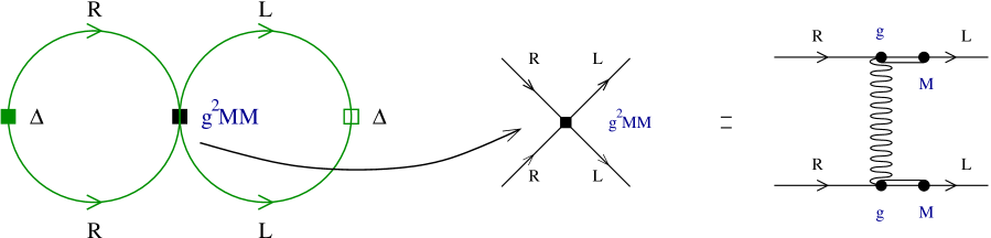
Figure 15: The left panel shows the diagram in the high density effective theory that contributes to the vacuum energy at order $O(M^{2})$. The right panel shows how the effective four-fermion vertex can be matched against a chirality violating scattering amplitude involving a hard gluon exchange.

Note that a factor $g^{2}$ in the vertex equ. (127) cancels against a factor $1/g$ that comes from a logarithmic $\log(\Delta)$ divergence in the superfluid density. Matching equ. (129) against equ. (118) we can determine the coefficients $A_{1,2,3}$. We find Son:1999cm ; Schafer:2001za

$$A_{1}=-A_{2}=\frac{3\Delta^{2}}{4\pi^{2}},\hskip 28.45274ptA_{3}=0.$$ (130)

We note that ${\cal E}\sim f_{\pi}^{2}\Delta^{2}(\Delta/p_{F})$ $[M^{2}/(p_{F}\Delta)]$ which shows that the coefficients $A_{i}$ are suppressed by $(\Delta/p_{F})$. The effective lagrangian equs. (121-127) can also be used to compute higher order terms in $M$. The dominant $O(M^{4})$ term is the effective chemical potential term equ. (126). Other $O(M^{4})$ terms are suppressed by additional powers of $(\Delta/p_{F})$.

IX.5 Instanton effects

In the CFL phase spontaneous chiral symmetry breaking is dominated by order parameters of the form $\langle(\bar{\psi}\psi)^{2}\rangle$ and as a consequence the coefficient of the linear mass term in the chiral lagrangian is suppressed as compared to the quadratic mass term. Indeed, the CFL phase has an approximate $(Z_{2})_{A}$ symmetry that forbids the linear mass term. The $(Z_{2})_{A}$ symmetry is broken by instantons. This means that in the CFL phase the quark-anti-quark condensate is induced by instantons.

We shall determine the coefficient $B$ of the linear mass term by computing the instanton induced shift in the vacuum energy. The corresponding diagram is shown in Fig. 16. In QCD with three flavors, the instanton induced interaction between quarks is given by 'tHooft:up ; Shifman:uw ; Schafer:1996wv

$${\cal L} = \int n(\rho,\mu)d\rho\,\frac{(2\pi\rho)^{6}\rho^{3}}{6N_{c}(N_{c}^{2}-1)}\epsilon_{f_{1}f_{2}f_{3}}\epsilon_{g_{1}g_{2}g_{3}}\left(\frac{2N_{c}+1}{2N_{c}+4}(\bar{\psi}_{R,f_{1}}\psi_{L,g_{1}})(\bar{\psi}_{R,f_{2}}\psi_{L,g_{2}})(\bar{\psi}_{R,f_{3}}\psi_{L,g_{3}})\right.$$ (131)

$$\mbox{}\left.-\frac{3}{8(N_{c}+2)}(\bar{\psi}_{R,f_{1}}\psi_{L,g_{1}})(\bar{\psi}_{R,f_{2}}\sigma_{\mu\nu}\psi_{L,g_{2}})(\bar{\psi}_{R,f_{3}}\sigma_{\mu\nu}\psi_{L,g_{3}})+(L\leftrightarrow R)\right).$$

Here, $\rho$ is the instanton size, $\mu$ is the quark chemical potential, $f_{i},g_{i}$ are flavor indices and $\sigma_{\mu\nu}=\frac{i}{2}[\gamma_{\mu},\gamma_{\nu}]$. The instanton size distribution $n(\rho,\mu)$ is given by

$$n(\rho,\mu) = C_{N}\ \left(\frac{8\pi^{2}}{g^{2}}\right)^{2N_{c}}\rho^{-5}\exp\left[-\frac{8\pi^{2}}{g(\rho)^{2}}\right]\exp\left[-N_{f}\rho^{2}\mu^{2}\right],$$ (134)

$$C_{N}\;=\;\frac{0.466\exp(-1.679N_{c})1.34^{N_{f}}}{(N_{c}-1)!(N_{c}-2)!}\,,$$

$$\frac{8\pi^{2}}{g^{2}(\rho)}\;=\;-b\log(\rho\Lambda),\hskip 28.45274ptb=\frac{11}{3}N_{c}-\frac{2}{3}N_{f}\,.$$

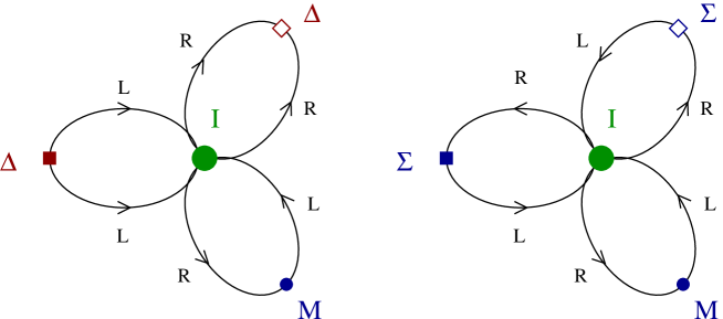
Figure 16: Instanton contribution to the $O(M)$ term in the vacuum energy. The diagram on the left shows the instanton term in the CFL phase at high baryon density. The squares are anomalous self energy insertions. The diagram on the right is the corresponding term in QCD at low baryon density. The squares are normal self energy insertions.

At zero density, the $\rho$ integral in equ. (134) is divergent at large $\rho$. This is the well-known infrared problem of the semi-classical approximation in QCD. At large chemical potential, however, large instantons are suppressed and the typical instanton size is $\rho\sim\mu^{-1}\ll\Lambda^{-1}$. We also note that at zero density the effective lagrangian equ. (131) is derived by computing $U(1)_{A}$ violating Greens functions in the limit $p\ll\rho^{-1}$. From a similar study at finite density one can show that at $\mu\neq 0$ equ. (131) has to be interpreted as an effective lagrangian for momenta in the vicinity of the Fermi surface $|\vec{p}|-p_{F}\ll\rho^{-1}\sim\mu$ Schafer:1998up ; Carter:1999mt ; Schafer:2002ty .

To linear order in the quark mass one of the three zero modes is lifted. We find

$${\cal L} = \int n(\rho,\mu)d\rho\,\frac{2(2\pi\rho)^{4}\rho^{3}}{4(N_{c}^{2}-1)}\epsilon_{f_{1}f_{2}f_{3}}\epsilon_{g_{1}g_{2}g_{3}}M_{f_{3}g_{3}}\left(\frac{2N_{c}-1}{2N_{c}}(\bar{\psi}_{R,f_{1}}\psi_{L,g_{1}})(\bar{\psi}_{R,f_{2}}\psi_{L,g_{2}})\right.$$

$$\hskip 28.45274pt\mbox{}\left.-\frac{1}{8N_{c}}(\bar{\psi}_{R,f_{1}}\sigma_{\mu\nu}\psi_{L,g_{1}})(\bar{\psi}_{R,f_{2}}\sigma_{\mu\nu}\psi_{L,g_{2}})+(M\leftrightarrow M^{\dagger},L\leftrightarrow R)\right),$$

We can now compute the expectation value of equ. (IX.5) in the CFL ground state Schafer:1999fe ; Rapp:1999qa ; Son:2001jm . To leading order in perturbative QCD we can use the mean field approximation $\langle(\bar{\psi}\psi)(\bar{\psi}\psi)\rangle\sim\langle\psi\psi\rangle\langle\bar{\psi}\bar{\psi}\rangle$. The instanton contribution to the vacuum energy density is

$${\cal E} = -\int n(\rho,\mu)d\rho\,\frac{16}{3}(\pi\rho)^{4}\rho^{3}\left[\frac{3\sqrt{2}\pi}{g}\Delta\left(\frac{\mu^{2}}{2\pi^{2}}\right)\right]^{2}{\rm Tr}\left[M+M^{\dagger}\right],$$ (136)

where we have used the perturbative result for the diquark condensate in the CFL phase

$$\langle\psi^{a}_{L,f}C\psi^{b}_{L,g}\rangle = -\langle\psi^{a}_{R,f}C\psi^{b}_{R,g}\rangle=\left(\delta^{a}_{f}\delta^{b}_{g}-\delta^{a}_{g}\delta^{b}_{f}\right)\Phi,$$

$$\Phi\,=\,\frac{3\sqrt{2}\pi}{g}\Delta\left(\frac{\mu^{2}}{2\pi^{2}}\right).$$

We note that for $M={\rm diag}(m_{u},m_{d},m_{s})$ the instanton contribution to the vacuum energy is indeed negative. Since the effective interaction involves both left and right-handed fermions the relative phase between the left and right-handed condensate in equ. (IX.5) is important. Instantons favor the state with $\langle\psi_{L}\psi_{L}\rangle=-\langle\psi_{R}\psi_{R}\rangle$ which is the parity even ground state. Equation (136) for the vacuum energy can be matched against the effective lagrangian equ. (118). We find

$$B=C_{N}\frac{8\pi^{4}}{3}\frac{\Gamma(6)}{3^{6}}\left[\frac{3\sqrt{2}\pi}{g}\Delta\left(\frac{\mu^{2}}{2\pi^{2}}\right)\right]^{2}\left(\frac{8\pi^{2}}{g^{2}}\right)^{6}\left(\frac{\Lambda}{\mu}\right)^{12}\Lambda^{-3},$$ (138)

where we have performed the integral over the instanton size $\rho$ using the one-loop beta function. The coefficient $B$ is related to the quark-anti-quark condensate, $\langle\bar{\psi}\psi\rangle=-2B$. We note that $B$ is indeed parametrically small, $B\sim(\Lambda/p_{F})^{8}$.

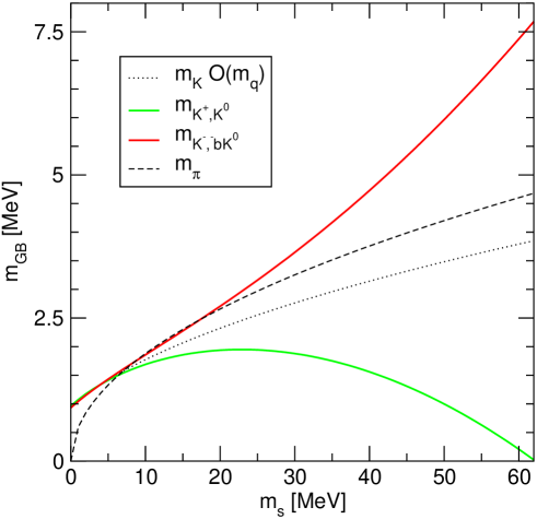
Figure 17: Goldstone boson masses in the CFL phase as a function of the strange quark mass, from Bedaque:2001je .

In QCD with three flavors chiral symmetry is broken both at small and at large density. The instantons contribution to the linear Goldstone boson mass term in the low density phase is shown in Fig. 16b. Again, the coefficient of the ${\rm Tr}(M\Sigma)$ term in the effective lagrangian is the instanton contribution to the quark condensate. There are strong arguments that instantons dominate chiral symmetry breaking in QCD at zero density, see Schafer:1996wv for a review. This raises the question whether the instanton mechanisms of Fig. 16a and b are continuously connected. In a simple mean field calculation it was found that there is a first order phase transition that separates instanton induced chiral symmetry breaking at low and high density Rapp:1999qa , but this question certainly deserves further study.

IX.6 Kaon condensation

Using the results discussed in the previous sections we can compute the masses of Goldstone bosons in the CFL phase. In Sect. IX.3 we argued that the expansion parameter in the chiral expansion of the Goldstone boson masses is $\delta=m^{2}/(p_{F}\Delta)$. The first term in this expansion comes from the $O(M^{2})$ term in equ. (IX.3), but the coefficients $A$ contain the additional small parameter $\epsilon=(\Delta/p_{F})$. In a combined expansion in $\delta$ and $\epsilon$ the $O(\epsilon\delta)$ mass term and the $O(\delta^{2})$ chemical potential term equ. (125) appear at the same order. Instanton effects are suppressed by extra powers of $(\Lambda/p_{F})$. To order $O(\epsilon\delta,\delta^{2})$ the masses of the flavored Goldstone bosons are

$$m_{\pi^{\pm}} = \mp\frac{m_{d}^{2}-m_{u}^{2}}{2p_{F}}+\left[\frac{4A}{f_{\pi}^{2}}(m_{u}+m_{d})m_{s}\right]^{1/2},$$

$$m_{K_{\pm}} = \mp\frac{m_{s}^{2}-m_{u}^{2}}{2p_{F}}+\left[\frac{4A}{f_{\pi}^{2}}m_{d}(m_{u}+m_{s})\right]^{1/2},$$ (139)

$$m_{K^{0},\bar{K}^{0}} = \mp\frac{m_{s}^{2}-m_{d}^{2}}{2p_{F}}+\left[\frac{4A}{f_{\pi}^{2}}m_{u}(m_{d}+m_{s})\right]^{1/2}.$$

Further studies of Goldstone boson properties in the CFL phase can be found in Rho:2000xf ; Hong:2000ei ; Manuel:2000wm ; Rho:2000ww ; Beane:2000ms . We observe that the pion masses are not strongly affected by the effective chemical potential $\mu_{s}=m_{s}^{2}/(2p_{F})$ but the masses of the $K^{+}$ and $K^{0}$ are substantially lowered while the $K^{-}$ and $\bar{K}^{0}$ are pushed up. As a result the $K^{+}$ and $K^{0}$ meson become massless if

$$\left.m_{s}\right|_{crit}=3.03\cdot m_{d}^{1/3}\Delta^{2/3},$$ (140)

see Fig. 17. For larger values of $m_{s}$ the kaon modes are unstable, signaling the formation of a kaon condensate.

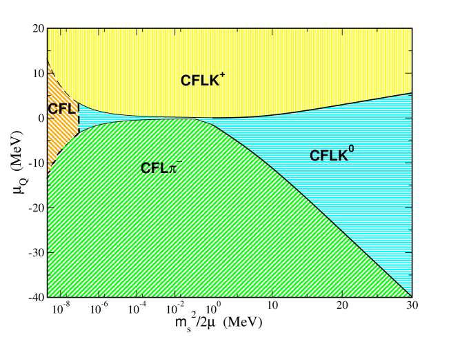
Figure 18: This figure shows the phase structure of CFL matter as a function of the strange quark mass $m_{s}$ and the lepton chemical potential $\mu_{Q}$, from Kaplan:2001qk .

Kaon condensation implies that the CFL ground state is reorganized. For simplicity, we consider the case of exact isospin symmetry $m_{u}=m_{d}\equiv m$. Kaon condensation can be studied using an ansatz of the form $\Sigma=\exp(i\alpha\lambda_{4})$. The vacuum energy is

$$V(\alpha)=-f_{\pi}^{2}\left(\frac{1}{2}\left(\frac{m_{s}^{2}-m^{2}}{2p_{F}}\right)^{2}\sin(\alpha)^{2}+(m_{K}^{0})^{2}(\cos(\alpha)-1)\right),$$ (141)

where $(m_{K}^{0})^{2}=(4A/f_{\pi}^{2})m_{u,d}(m_{u,d}+m_{s})$ is the $O(M^{2})$ kaon mass in the limit of exact isospin symmetry. Minimizing the vacuum energy we obtain $\alpha=0$ if $m_{s}^{2}/(2p_{F})<m_{K}^{0}$ and $\cos(\alpha)=(m_{K}^{0})^{2}/\mu_{s}^{2}$ with $\mu_{s}=m_{s}^{2}/(2p_{F})$ if $\mu_{s}>m_{K}^{0}$. In the kaon condensed phase $SU(2)_{I}\times U(1)_{Y}$ is spontaneously broken to $U(1)_{Q}$. This coincides with the symmetry breaking pattern in the electroweak sector of the standard model. Kaon condensation also provides an interesting realization of Goldstone’s theorem. Even though the number of broken generators is three, the number of Goldstone bosons is only two. This is related to the fact that one of the Goldstone modes has a quadratic dispersion relation Miransky:2001tw ; Schafer:2001bq .

The hypercharge density in the kaon condensed phase is given by

$$n_{Y}=f_{\pi}^{2}\mu_{s}\left(1-\frac{(m_{K}^{0})^{4}}{\mu_{s}^{4}}\right).$$ (142)

This result is exactly analogous to the behavior of the charge density in the case of the dilute Bose gas, equ. (26), and $N_{c}=2$ QCD, equ. (100). We observe that within the range of validity of the effective theory, $\mu_{s}<\Delta$, the hypercharge density satisfies $n_{Y}<\Delta p_{F}^{2}/(2\pi^{2})$. This means that the number of condensed kaons is bounded by the number of particles contained within a strip of width $\Delta$ around the Fermi surface. The maximum hypercharge density allowed by the effective theory corresponds to the case that essentially all strange quarks have been removed from the CFL wave function. This raises the question whether the CFL-2SC transition might be more complicated than what is suggested by the simple BCS model discussed in Sect. IX.2, see Fig. 11.

In the limit of exact isospin symmetry the $K^{0}$ and $K^{+}$ condensed phases are degenerate. If charge neutrality is imposed then the $K^{0}$ condensed phase is preferred. The effective lagrangian equ. (IX.3) can be used to study a number of question related to the structure and the low energy properties of the CFL phase. The phase structure as a function of the strange quark mass and non-zero lepton chemical potentials was studied by Kaplan and Reddy Kaplan:2001qk , see Fig. 18. Other investigations have focused on the role of defects such as $K^{0}$ vortices Kaplan:2001hh ; Buckley:2002ur , as well as transport properties such as neutrino emissivity and thermal conductivity Reddy:2002xc ; Jaikumar:2002vg ; Shovkovy:2002kv .

X Conclusion: The many phases of QCD

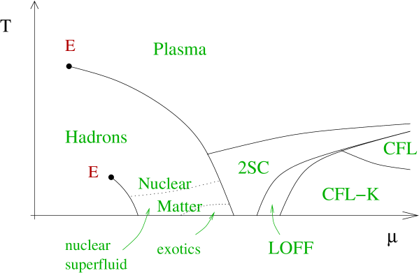
Figure 19: Conjectured phase diagram of three flavor QCD with realistic quark masses.

There are many issues in QCD at finite density that remain to be addressed. First of all it would clearly be of great help if some of the ideas discussed in these lectures could be tested using numerical simulations on the lattice. While some progress in this direction has been made, the most interesting regime of the phase diagram remains unexplored. Even more importantly, we have to find experimental or observational constraints on the properties of quark matter. In Sect. VI we mentioned the possibility of observing the QCD tri-critical in relativistic heavy ion collisions. Observational constraints on the properties of dense cold matter can be obtained from neutron stars. We refer the reader to Reddy:2002ri for a recent review and a guide to the literature.

On the more theoretical side we would like to improve our understanding of the phase diagram of QCD for realistic values of the strange quark mass. In Figs. 6,7,9 we have shown proposed phase diagrams for idealized versions of QCD. A conjectured phase diagram for QCD with three flavors and realistic quark masses is shown in Fig. 19. The reader will recognize many of the phases that we have discussed in the previous sections. However, from our discussion it is also clear that many of the phases, the transition lines, and the order of the transition are just guesses, based on mean-field or weak coupling arguments. Eventually, this problem will have to be resolved using observations and numerical simulations. In the mean time, however, we would also like to improve and systematize the theoretical approaches. This should be possible in both the limit of high and low density, using, respectively, weak coupling QCD and nuclear effective field theory.

Acknowledgments: I would like to thank the organizers of the BARC workshop on “Mesons and Quarks” for their hospitality. I would also like to acknowledge the many discussions on dense QCD I have had with friends and collaborators over the years. I would like to thank, in particular, Mark Alford, Paulo Bedaque, Krishna Rajagopal, Francesco Sannino, Dam Son, Edward Shuryak, Misha Stephanov, and Frank Wilczek. This work was supported in part by a US DOE OJI grant. The write-up was completed during the INT workshop on “The first three years of running at RHIC”. I would like to thank the INT in Seattle for hospitality.

References

- (1) E. V. Shuryak, The QCD vacuum, hadrons, and the superdense matter, World Scientific, Singapore (1988).
- (2) J. Kapusta, Finite temperature field theory, Cambridge University Press, Cambridge (1989).
- (3) M. LeBellac, Thermal Field Theory, Cambridge University Press, Cambridge (1996).
- (4) K. Rajagopal and F. Wilczek, The condensed matter physics of QCD, in: Festschrift in honor of B.L. Ioffe, ’At the Frontier of Particle Physics / Handbook of QCD’, M. Shifman, ed., World Scientific, Singapore, hep-ph/0011333.
- (5) M. G. Alford, Ann. Rev. Nucl. Part. Sci. 51, 131 (2001) [hep-ph/0102047].
- (6) G. Nardulli, Riv. Nuovo Cim. 25N3, 1 (2002) [hep-ph/0202037].
- (7) S. Reddy, Acta Phys. Polon. B 33, 4101 (2002) [nucl-th/0211045].
- (8) A. A. Abrikosov, L. P. Gorkov and I. E. Dzyaloshinski, Methods of quantum field theory in statistical physics, Prentice-Hall, Englewood Cliffs, N.J. (1963).
- (9) H. W. Hammer and R. J. Furnstahl, Nucl. Phys. A 678, 277 (2000) [nucl-th/0004043].
- (10) K. Huang and C. N. Yang, Phys. Rev. 105, 767 (1957).
- (11) T. D. Lee and C. N. Yang, Phys. Rev. 105, 1119 (1957).
- (12) A. L. Fetter and J. D. Walecka, Quantum theory of many particle systems, McGraw Hill, New York (1971).
- (13) L. Platter, H. W. Hammer and U. G. Meissner, Nucl. Phys. A 714, 250 (2003) [nucl-th/0208057].
- (14) L. D. Landau, E. M. Lifshitz, Physical Kinetics (Course of Theoretical Physics, Vol.X), Pergamon Press (1981).
- (15) V. N. Popov, Functional integrals and collective excitations, Cambridge University Press (1987).
- (16) D. T. Son, preprint, hep-ph/0204199.
- (17) R. Shankar, Rev. Mod. Phys. 66, 129 (1994).
- (18) J. Polchinski, Effective field theory and the Fermi surface, Lectures presented at TASI 92, Boulder, CO, hep-th/9210046.
- (19) T. Papenbrock and G. F. Bertsch, Phys. Rev. C 59, 2052 (1999) [nucl-th/9811077].
- (20) V. A. Khodel, V. V. Khodel, and J. W. Clark, Nucl. Phys. A598 (1996) 390.
- (21) S. Weinberg, Nucl. Phys. B413, 567 (1994).
- (22) D. Pines, The theory of quantum liquids, Addison-Wesley, Menlo Park (1966).
- (23) G. Baym, C. Pethick, Landau Fermi Liquid Theory, Wiley, New York (1991).
- (24) S. Weinberg, The quantum theory of fields, vol. II, Cambridge University Press (1995).
- (25) P. W. Anderson, Basic notions of condensed matter physics, Benjamin/Cummings Pub. Co., Menlo Park, CA (1984).
- (26) Z. Fodor and S. D. Katz, JHEP 0203, 014 (2002) [hep-lat/0106002].
- (27) P. de Forcrand and O. Philipsen, Nucl. Phys. B 642, 290 (2002) [hep-lat/0205016].
- (28) C. R. Allton et al., Phys. Rev. D 66, 074507 (2002) [hep-lat/0204010].
- (29) C. Vafa and E. Witten, Nucl. Phys. B 234, 173 (1984).
- (30) C. Vafa and E. Witten, Phys. Rev. Lett. 53, 535 (1984).
- (31) J. C. Collins and M. J. Perry, Phys. Rev. Lett. 34, 1353 (1975).
- (32) B. A. Freedman and L. D. McLerran, Phys. Rev. D 16, 1130 (1977).
- (33) E. S. Fraga, R. D. Pisarski and J. Schaffner-Bielich, Phys. Rev. D 63, 121702 (2001) [hep-ph/0101143].
- (34) T. Holstein, A. E. Norton, P. Pincus, Phys. Rev. B8, 2649 (1973).
- (35) M. Yu. Reizer, Phys. Rev. B 40, 11571 (1989).
- (36) G. Baym, H. Monien, C. J. Pethick and D. G. Ravenhall, Phys. Rev. Lett. 64, 1867 (1990).
- (37) C. Manuel, Phys. Rev. D 62, 114008 (2000) [hep-ph/0006106].
- (38) D. Boyanovsky and H. J. de Vega, Phys. Rev. D 63, 034016 (2001) [hep-ph/0009172].
- (39) W. E. Brown, J. T. Liu and H. C. Ren, Phys. Rev. D 62, 054016 (2000) [hep-ph/9912409].
- (40) S. C. Frautschi, Asymptotic freedom and color superconductivity in dense quark matter, in: Proceedings of the Workshop on Hadronic Matter at Extreme Energy Density, N. Cabibbo, Editor, Erice, Italy (1978).
- (41) B. C. Barrois, Nucl. Phys. B129, 390 (1977).
- (42) F. Barrois, Nonperturbative effects in dense quark matter, Ph.D. thesis, Caltech, UMI 79-04847-mc (microfiche).
- (43) D. Bailin and A. Love, Phys. Rept. 107, 325 (1984).
- (44) M. Alford, K. Rajagopal and F. Wilczek, Phys. Lett. B422, 247 (1998) [hep-ph/9711395].
- (45) R. Rapp, T. Schäfer, E. V. Shuryak and M. Velkovsky, Phys. Rev. Lett. 81, 53 (1998) [hep-ph/9711396].
- (46) R. D. Pisarski and F. Wilczek, Phys. Rev. D 29, 338 (1984).
- (47) A. Barducci, R. Casalbuoni, S. De Curtis, R. Gatto and G. Pettini, Phys. Lett. B 231, 463 (1989).
- (48) A. Barducci, R. Casalbuoni, S. De Curtis, R. Gatto and G. Pettini, Phys. Rev. D 41, 1610 (1990).
- (49) A. Barducci, R. Casalbuoni, G. Pettini and R. Gatto, Phys. Rev. D 49, 426 (1994).
- (50) J. Berges and K. Rajagopal, Nucl. Phys. B 538, 215 (1999) [hep-ph/9804233].
- (51) M. A. Halasz, A. D. Jackson, R. E. Shrock, M. A. Stephanov and J. J. Verbaarschot, Phys. Rev. D 58, 096007 (1998) [hep-ph/9804290].
- (52) M. Stephanov, K. Rajagopal and E. V. Shuryak, Phys. Rev. Lett. 81, 4816 (1998) [hep-ph/9806219].
- (53) M. Kitazawa, T. Koide, T. Kunihiro and Y. Nemoto, Prog. Theor. Phys. 108, 929 (2002) [hep-ph/0207255].
- (54) N. Evans, S. D. Hsu and M. Schwetz, Nucl. Phys. B551, 275 (1999) [hep-ph/9808444].
- (55) T. Schäfer and F. Wilczek, Phys. Lett. B450, 325 (1999) [hep-ph/9810509].
- (56) T. Schäfer, Phys. Rev. D62, 094007 (2000) [hep-ph/0006034].
- (57) D. T. Son, Phys. Rev. D59, 094019 (1999) [hep-ph/9812287].
- (58) T. Schäfer and F. Wilczek, Phys. Rev. D60, 114033 (1999) [hep-ph/9906512].
- (59) R. D. Pisarski and D. H. Rischke, Phys. Rev. D61, 074017 (2000) [nucl-th/9910056].
- (60) D. K. Hong, V. A. Miransky, I. A. Shovkovy and L. C. Wijewardhana, Phys. Rev. D61, 056001 (2000) [hep-ph/9906478].
- (61) W. E. Brown, J. T. Liu and H. c. Ren, Phys. Rev. D 61, 114012 (2000) [hep-ph/9908248].
- (62) J. P. Blaizot and J. Y. Ollitrault, Phys. Rev. D 48, 1390 (1993) [hep-th/9303070].
- (63) C. Manuel, Phys. Rev. D 53, 5866 (1996) [hep-ph/9512365].
- (64) D. H. Rischke, Phys. Rev. D 62, 034007 (2000) [nucl-th/0001040].
- (65) Q. Wang and D. H. Rischke, Phys. Rev. D 65, 054005 (2002) [nucl-th/0110016].
- (66) D. H. Rischke, D. T. Son and M. A. Stephanov, Phys. Rev. Lett. 87, 062001 (2001) [hep-ph/0011379].
- (67) M. G. Alford, J. A. Bowers, J. M. Cheyne and G. A. Cowan, Phys. Rev. D 67, 054018 (2003) [hep-ph/0210106].
- (68) T. Schäfer, Nucl. Phys. B 575, 269 (2000) [hep-ph/9909574].
- (69) N. Evans, J. Hormuzdiar, S. D. Hsu and M. Schwetz, Nucl. Phys. B 581, 391 (2000) [hep-ph/9910313].
- (70) M. Alford, K. Rajagopal and F. Wilczek, Nucl. Phys. B537, 443 (1999) [hep-ph/9804403].
- (71) T. Schäfer and F. Wilczek, Phys. Rev. Lett. 82, 3956 (1999) [hep-ph/9811473].
- (72) G. ’t Hooft, in: Recent developments in gauge theories, G. ’t Hooft, editor, Plenum Press, New York (1980).
- (73) M. Peskin, in: Recent advances in field theory and statistical mechanics, Les Houches 1982, J. B. Zuber and R. Stora, editors, North Holland, Amsterdam (1984).
- (74) F. Sannino, Phys. Lett. B 480, 280 (2000) [hep-ph/0002277].
- (75) F. Sannino, preprint, hep-ph/0301035.
- (76) M. E. Peskin, Nucl. Phys. B 175, 197 (1980).
- (77) J. B. Kogut, M. A. Stephanov and D. Toublan, Phys. Lett. B 464, 183 (1999) [hep-ph/9906346].
- (78) J. B. Kogut, M. A. Stephanov, D. Toublan, J. J. Verbaarschot and A. Zhitnitsky, Nucl. Phys. B 582, 477 (2000) [hep-ph/0001171].
- (79) J. B. Kogut, D. Toublan and D. K. Sinclair, Nucl. Phys. B 642, 181 (2002) [hep-lat/0205019].
- (80) T. Schäfer, Phys. Rev. D 57, 3950 (1998) [hep-ph/9708256].
- (81) J. T. Lenaghan, F. Sannino and K. Splittorff, Phys. Rev. D 65, 054002 (2002) [hep-ph/0107099].
- (82) F. Sannino, Phys. Rev. D 67, 054006 (2003) [hep-ph/0211367].
- (83) K. Splittorff, D. Toublan and J. J. Verbaarschot, Nucl. Phys. B 639, 524 (2002) [hep-ph/0204076].
- (84) T. Schäfer, Phys. Rev. D 67, 074502 (2003) [hep-lat/0211035].
- (85) M. G. Alford, A. Kapustin and F. Wilczek, Phys. Rev. D 59, 054502 (1999) [hep-lat/9807039].
- (86) D. T. Son and M. A. Stephanov, Phys. Rev. Lett. 86, 592 (2001) [hep-ph/0005225].
- (87) D. V. Deryagin, D. Yu. Grigoriev, and V. A. Rubakov, Int. J. Mod. Phys. A7, 659 (1992).
- (88) G. Gruner, Density waves in solids, Addison-Wesley Pub. Co (1994).
- (89) E. Shuster and D. T. Son, Nucl. Phys. B 573, 434 (2000) [hep-ph/9905448].
- (90) R. Rapp, E. V. Shuryak and I. Zahed, Phys. Rev. D 63, 034008 (2001) [hep-ph/0008207].
- (91) T. Schäfer and F. Wilczek, Phys. Rev. D60, 074014 (1999) [hep-ph/9903503].
- (92) M. Alford, J. Berges and K. Rajagopal, Nucl. Phys. B558, 219 (1999) [hep-ph/9903502].
- (93) R. Rapp, T. Schäfer, E. V. Shuryak, and M. Velkovsky, Annals Phys. 280, 35 (2000), [hep-ph/9904353].
- (94) P. Bedaque, Nucl. Phys. A 697, 569 (2002) [hep-ph/9910247].
- (95) M. G. Alford, J. Bowers and K. Rajagopal, Phys. Rev. D 63, 074016 (2001) [hep-ph/0008208].
- (96) T. Schäfer, Phys. Rev. Lett. 85, 5531 (2000) [nucl-th/0007021].
- (97) P. F. Bedaque and T. Schäfer, Nucl. Phys. A697, 802 (2002) [hep-ph/0105150].
- (98) D. B. Kaplan and S. Reddy, Phys. Rev. D 65, 054042 (2002) [hep-ph/0107265].
- (99) R. Casalbuoni, F. De Fazio, R. Gatto, G. Nardulli and M. Ruggieri, Phys. Lett. B 547, 229 (2002) [hep-ph/0209105].
- (100) T. D. Fugleberg, Phys. Rev. D 67, 034013 (2003) [hep-ph/0206033].
- (101) R. Casalbuoni, R. Gatto, G. Nardulli and M. Ruggieri, preprint, hep-ph/0302077.
- (102) A. W. Steiner, S. Reddy and M. Prakash, Phys. Rev. D 66, 094007 (2002) [hep-ph/0205201].
- (103) M. Alford and K. Rajagopal, JHEP 0206, 031 (2002) [hep-ph/0204001].
- (104) F. Neumann, M. Buballa and M. Oertel, Nucl. Phys. A 714, 481 (2003) [hep-ph/0210078].
- (105) K. Rajagopal and F. Wilczek, Phys. Rev. Lett. 86, 3492 (2001) [hep-ph/0012039].
- (106) I. Shovkovy and M. Huang, preprint, hep-ph/0302142.
- (107) E. Gubankova, W. V. Liu and F. Wilczek, preprint, hep-ph/0304016.
- (108) A. I. Larkin and Yu. N. Ovchinikov, Zh. Eksp. Theor. Fiz. 47, 1136 (1964); engl. translation: Sov. Phys. JETP 20, 762 (1965).
- (109) P. Fulde and A. Ferrell, Phys. Rev. 145, A550 (1964).
- (110) A. A. Abrikosov, Fundamentals of the theory of metals, North-Holland, Amsterdam (1988).
- (111) J. A. Bowers and K. Rajagopal, Phys. Rev. D 66, 065002 (2002) [hep-ph/0204079].
- (112) R. Casalbuoni and D. Gatto, Phys. Lett. B464, 111 (1999) [hep-ph/9908227].
- (113) D. K. Hong, Phys. Lett. B 473, 118 (2000) [hep-ph/981251].
- (114) D. K. Hong, Nucl. Phys. B 582, 451 (2000) [hep-ph/9905523].
- (115) S. R. Beane, P. F. Bedaque and M. J. Savage, Phys. Lett. B 483, 131 (2000) [hep-ph/0002209].
- (116) T. Schäfer, Phys. Rev. D 65, 074006 (2002) [hep-ph/0109052].
- (117) D. T. Son and M. Stephanov, Phys. Rev. D61, 074012 (2000) [hep-ph/9910491], erratum: hep-ph/0004095.
- (118) K. Zarembo, Phys. Rev. D 62, 054003 (2000) [hep-ph/0002123].
- (119) V. A. Miransky, I. A. Shovkovy and L. C. Wijewardhana, Phys. Rev. D 63, 056005 (2001) [hep-ph/0009173].
- (120) G. ’t Hooft, Phys. Rev. Lett. 37, 8 (1976).
- (121) M. A. Shifman, A. I. Vainshtein and V. I. Zakharov, Nucl. Phys. B 163, 46 (1980).
- (122) T. Schäfer and E. V. Shuryak, Rev. Mod. Phys. 70, 323 (1998) [hep-ph/9610451].
- (123) G. W. Carter and D. I. Diakonov, Nucl. Phys. A 661, 625 (1999), [hep-ph/9908314].
- (124) T. Schäfer, Phys. Rev. D 65, 094033 (2002) [hep-ph/0201189].
- (125) D. T. Son, M. A. Stephanov and A. R. Zhitnitsky, Phys. Lett. B 510, 167 (2001) [hep-ph/0103099].
- (126) M. Rho, A. Wirzba, and I. Zahed, Phys. Lett. B473, 126 (2000) [hep-ph/9910550].
- (127) D. K. Hong, T. Lee, and D. Min, Phys. Lett. B477, 137 (2000) [hep-ph/9912531].
- (128) C. Manuel and M. H. Tytgat, Phys. Lett. B479, 190 (2000) [hep-ph/0001095].
- (129) M. Rho, E. Shuryak, A. Wirzba and I. Zahed, Nucl. Phys. A 676, 273 (2000) [hep-ph/0001104].
- (130) V. A. Miransky and I. A. Shovkovy, Phys. Rev. Lett. 88, 111601 (2002) [hep-ph/0108178].
- (131) T. Schäfer, D. T. Son, M. A. Stephanov, D. Toublan and J. J. Verbaarschot, Phys. Lett. B 522, 67 (2001) [hep-ph/0108210].
- (132) D. B. Kaplan and S. Reddy, Phys. Rev. Lett. 88, 132302 (2002) [hep-ph/0109256].
- (133) K. B. Buckley and A. R. Zhitnitsky, JHEP 0208, 013 (2002) [hep-ph/0204064].
- (134) S. Reddy, M. Sadzikowski and M. Tachibana, Nucl. Phys. A 714, 337 (2003) [nucl-th/0203011].
- (135) P. Jaikumar, M. Prakash and T. Schäfer, Phys. Rev. D 66, 063003 (2002) [astro-ph/0203088].
- (136) I. A. Shovkovy and P. J. Ellis, Phys. Rev. C 66, 015802 (2002) [hep-ph/0204132].