Inflationary Attractor from Tachyonic Matter

Abstract

We study the complete evolution of a flat and homogeneous universe dominated by tachyonic matter. We demonstrate the attractor behaviour of the tachyonic inflation using the Hamilton-Jacobi formalism. We else obtain analytical approximations to the trajectories of the tachyon field in different regions. The numerical calculation shows that an initial non-vanishing momentum does not prevent the onset of inflation. The slow-rolling solution is an attractor.

I Introduction

The study of non-BPS objects such as non-BPS branes, brane-antibrane configurations and spacelike branes has recently attracted great attention given its implications for string/M-theory and cosmology. The tachyon field associated with unstable D-branes, might be responsible for cosmological inflation at early epochs due to tachyon condensation near the top of the effective potential DDD , and could contribute to some new form of cosmological dark matter at late times SEN . Several authors have investigated the process of rolling of the tachyon in the cosmological background GWG ; GS . In the slow roll limit in FRW cosmology, the exact solution of tachyonic inflation with exponential potential is found MPT .

A question which has not yet been addressed in the literature on tachyonic inflation is the issue of constraints on the phase space of initial conditions for inflation which arise when one takes into account the fact that in the context of cosmology the momenta of the tachyon field cannot be neglected in the early universe. For models of the type of chaotic inflation, the work of HAF shows that most of the energetically accessible field value space give rise to a sufficiently long period of slow roll inflation. However, for models of the type of new inflation, allowing for non-vanishing initial field momenta may dramatically reduce the phase space of initial conditions for which successful inflation results, and the attractor is the slow rolling solution DSG .

In this paper we investigate the constrains on the initial conditions of inflation with tachyon rolling down an exponential potential in phase space required for successful inflation. We demonstrate the attractor behaviour of the tachyonic inflation using the Hamilton-Jacobi formalism. We else use an explicitly numerical computation of the phase space trajectories and obtain analytical approximations to the trajectories of the tachyon in different regions. We find that in phase space there exists a curve that attracts most of the solutions.

II Tachyonic Matter Cosmology

According to Sen SEN , the effective action of the tachyon field in the Born-Infeld form can be written as

$$S=\int d^{4}x\sqrt{-g}\left(\frac{1}{2\kappa^{2}}R+V(T)\sqrt{1+g^{\mu\nu}\partial_{\mu}T\partial_{\nu}T}\right)$$ (1)

where T is the tachyon field minimally coupled to gravity. The rolling tachyon in a spatially flat FRW cosmological model can be described by a fluid with a positive energy density $\rho$ and a negative pressure $P$ given by

$$\rho = \frac{V(T)}{\sqrt{1-\dot{T}^{2}}},$$ (2)

$$P = -V(T)\sqrt{1-\dot{T}^{2}},$$ (3)

Thus

$$\omega=\frac{P}{\rho}=-(1-\dot{T}^{2})$$ (4)

Note that $-1\leq\omega\leq 0$, and a universe dominated by this rolling tachyonic matter will smoothly evolve from a phase of accelerating expansion to a phase dominated by a non-relativistic fluid GWG . The evolution equation of the tachyon field minimally coupled to gravity, and the Friedmann equation are

$$\frac{\dot{\Pi}}{1-\Pi^{2}}+3H\Pi+\frac{V^{\prime}(T)}{V(T)}=0,$$ (5)

$$H^{2}=\frac{\kappa^{2}}{3}\frac{V(T)}{\sqrt{1-\Pi^{2}}},$$ (6)

where $\Pi\equiv\dot{T}$ denotes the velocity of tachyon. A universe dominated by tachyon field would go under accelerating expansion as long as $\Pi^{2}<2/3$ which is very different from the condition of inflation for non-tachyonic field, $\dot{\phi}^{2}<V(\phi)$. The tachyon potential $V(T)\to 0$ as $T\to\infty$, but its exact form is not known at present AAGS . Sen has argued that the qualitative dynamics of string theory tachyons can be described by (1) with the exponential potential SENN

$$V(T)=V_{0}e^{-\alpha T},$$ (7)

where $\alpha$ is the tachyon mass. The cosmological aspects of rolling tachyon with exponential potential are investigated MPT . In what follows we will consider (1) with exponential potential in purely phenomenological context without claiming any identification of $T$ with the string tachyon field.

III Inflationary Attractor

The Hamilton-Jacobi formulation SB is a powerful way of rewriting the equations of motion, which allows an easier derivation of many inflation results. We concentrate here on the homogeneous situation as applied to spatially flat cosmologies, and demonstrate the attractor behaviour of the tachyonic inflation using the Hamilton-Jacobi formalism LPB .

Differentiating Eq.(6) with respect to $t$ and substituting in Eq.(5) gives

$$\dot{T}=-\frac{2}{3}\frac{H^{\prime}(T)}{H^{2}(T)}$$ (8)

where primes denote derivatives with respect to the tachyon field $T$, which gives the relation between $T$ and $t$. This allows us to write the Friedmann equation in the first-order form

$$[H^{\prime}(T)]^{2}-\frac{9}{4}H^{4}(T)=-\frac{\kappa^{4}}{4}V^{2}(T)$$ (9)

Eq.(9) is the Hamilton-Jacobi equation. It allows us to consider $H(T)$, rather than $V(T)$, as the fundamental quantity to be specified. Suppose $H_{0}(T)$ is any solution to Eq.(9), which can be either inflationary or non-inflationary. Add to this a linear homogeneous perturbation $\delta H(T)$; the attractor condition will be satisfied if it becomes small as $T$ increases. Substituting $H(T)=H_{0}(T)+\delta H(T)$ into Eq.(9) and linearizing, we find that the perturbation obeys

$$H_{0}^{\prime}\delta H^{\prime}\simeq\frac{9}{2}H_{0}^{3}\delta H$$ (10)

which has the general solution

$$\delta H(T)=\delta H(T_{i})\exp\left(\frac{9}{2}\int_{T_{i}}^{T}\frac{H_{0}^{3}(T)}{H_{0}^{\prime}(T)}dT\right)$$ (11)

where $\delta H(T_{i})$ is the value at some initial point $T_{i}$. Because $H^{\prime}_{0}$ and $dT$ have opposing signs, the integrand within the exponential term is negative definite, and hence all linear perturbations do indeed die away. If there is an inflationary solution, all linear perturbations approach it at least exponentially fast as the tachyon field rolls.

IV Phase Portrait and Cosmological Evolution

We choose different initial conditions $T$, in the range $T\geq 0$, and $\Pi$ in the range $0\leq\Pi\leq 1$ and we obtain the phase portrait in the $(T,\Pi)$ plane. Figure 1 shows that there exists a curve that attracts most of the trajectories, in the $(x,y)$ plane where $x=\alpha T$ and $y=\Pi$ are dimensionless coordinates. The initial kinetic term decays rapidly and does not prevent the onset of inflation.

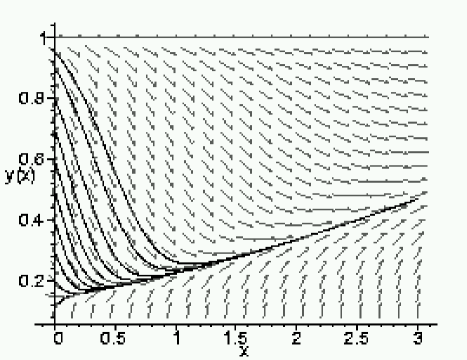
Figure 1: Phase portrait for tachyonic cosmology.

The behavior of the trajectories can be also analyzed analytically. To understand the evolution of the tachyon field we define two regions $P$ and $K$ in the $(T,\Pi)$ plane as indicated in Figure 2. The region $P$ is the region where the potential dominates over the energy density, and the region $K$ is the region where the kinetic energy dominates.

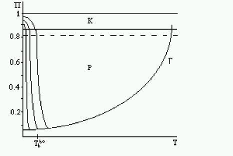
Figure 2: Sketch of the different regions in the ($T,\Pi$) phase plane.

Curve $\Gamma$. This curve describes the slow rolling solution where the evolution Eq. (5) and the Friedman Eq.(6) in expanding universe can be approximated by

$$3H\Pi+\frac{V^{\prime}(T)}{V(T)}=0,$$ (12)

$$H^{2}=\frac{\kappa^{2}}{3}V(T),$$ (13)

from which it follows that

$$\Pi = \frac{\alpha}{3\beta}e^{\frac{\alpha}{2}T}$$ (14)

$$T = \frac{2}{\alpha}\ln{\left(\frac{3\beta}{\alpha}\Pi\right)}$$ (15)

where $\beta\equiv\sqrt{\kappa^{2}V_{0}/3}$. The expression for the number $N$ of e-foldings of inflation can be written as

$$N=\ln{\frac{a_{e}}{a_{b}}}=\kappa^{2}\int_{T_{e}}^{T_{b}}\frac{V^{2}}{V^{\prime\prime}}dT=\left.\frac{\kappa^{2}}{\alpha^{2}}V(T)\right|_{T_{e}}^{T_{b}},$$ (16)

where $T_{b}$ is the value of the field at the point where it reaches curve $\Gamma$ and $T_{e}$ is the value of the field at the end of the slow rolling phase. In order to obtain enough e-foldings of slow roll inflation the value of $T_{b}$ for such a trajectory must satisfy

$$0\leq T_{b}<T_{b}^{60}$$ (17)

where $T_{b}^{60}$ is calculated from Eq.(16) with $N=60$.

Region $P$. In this region, the potential dominates over the energy density. The potential force $V^{\prime}(T)$ is negligible compared to the friction term since the friction coefficient is proportional to the potential. The evolution Eq.(5) and Friedman Eq.(6) are approximately

$$\dot{\Pi}+3H\Pi=0$$ (18)

$$H^{2}=\frac{\kappa^{2}}{3}V(T)$$ (19)

so that

$$\Pi = \Pi_{pk}-\frac{6\beta}{\alpha}\left(e^{-\frac{\alpha}{2}T_{pk}}-e^{-\frac{\alpha}{2}T}\right)$$ (20)

$$T = -\frac{2}{\alpha}\ln{\left[e^{-\frac{\alpha}{2}T_{pk}}-\frac{\alpha}{6\beta}\left(\Pi_{pk}-\Pi\right)\right]}$$ (21)

where $T_{pk}$ and $\Pi_{pk}$ are the values at the boundary between region $P$ and region $K$. Let us now denote by $T_{b}$ and $\Pi_{b}$ the values of the inflaton and its momentum when the trajectory reaches the slow roll curve.

$$T_{b}=-\frac{2}{\alpha}\ln{\left[e^{-\frac{\alpha}{2}T_{pk}}-\frac{\alpha}{6\beta}\Pi_{pk}\right]}$$ (22)

where we have neglected $\Pi_{b}$ since it is exponentially smaller than $\Pi_{pk}$. In general the unconventional forms of the tachyonic energy density and pressure make the cosmology with tachyon field differ from that with a normal scalar field, and make it difficult to separate kinetic term from potential term. We assume that $V(T)$ and $V(T)(\frac{1}{\sqrt{(1-\dot{T}^{2})}}-1)$ are regarded as potential and kinetic term respectively. Therefore, the boundary value between region $P$ and region $S$ is $\Pi_{pk}=\frac{\sqrt{3}}{2}$. So

$$T_{b}=-\frac{2}{\alpha}\ln{\left[e^{-\frac{\alpha}{2}T_{pk}}-\frac{\alpha}{4\sqrt{3}\beta}\right]}$$ (23)

To lead to sufficient inflation, from (17) such initial conditions must satisfy

$$-\frac{2}{\alpha}\ln{\left[e^{-\frac{\alpha}{2}T_{pk}}-\frac{\alpha}{4\sqrt{3}\beta}\right]}<T_{b}^{60}$$ (24)

Region $K$. It is the region of kinetic energy domination where $V^{\prime}(T)$ is negligible compared to the friction term and (5) and (6) become

$$\frac{\dot{\Pi}}{1-\Pi^{2}}+3H\Pi=0$$ (25)

$$H^{2}=\frac{\kappa^{2}}{3}\frac{V(T)}{\sqrt{1-\Pi^{2}}}$$ (26)

These can be integrated and we find:

$$\Pi_{2}F_{1}\left(\frac{1}{2},\frac{3}{4},\frac{3}{2},\Pi^{2}\right) = \Pi_{pk2}F_{1}\left(\frac{1}{2},\frac{3}{4},\frac{3}{2},\Pi_{pk}^{2}\right)$$ (27)

$$-\left.\frac{6\beta}{\alpha}e^{-\frac{\alpha}{2}T}\right|_{T}^{T_{pk}}$$

$$T=-\frac{2}{\alpha}\ln{\left[e^{-\frac{\alpha}{2}T_{pk}}-\left.\frac{\alpha}{6\beta}\Pi_{2}F_{1}\left(\frac{1}{2},\frac{3}{4},\frac{3}{2},\Pi^{2}\right)\right|_{\Pi}^{\Pi_{pk}}\right]}$$ (28)

where ${}_{2}F_{1}\left(\frac{1}{2},\frac{3}{4},\frac{3}{2},\Pi^{2}\right)$ is Gauss hypergeometric function.

V Conclusions and Discussions

To demonstrate the attractor behaviour of the tachyonic inflation, We use the Hamilton-Jacobi formalism, which greatly simplifies the analysis. Adding to any solution to Eq.(9) a linear homogeneous perturbation, we find the perturbation die away exponentially. The attractor behaviour indicates that, regardless of initial conditions, the late-time solutions are the same up to a time shift, which cannot be measured LMS . We else use an explicitly numerical computation of the phase space trajectories and obtain analytical approximations to the trajectories of the tachyon in different regions. One can easily verify from Figure 1 and Figure 2 that these approximations are in very good agreement with the numerical results, and that the slow rolling solution is the late-time attractor. Although the initial kinetic term decays rapidly and does not prevent the onset of inflation, allowing for non-vanishing initial field momenta around $T=0$ may dramatically reduce the phase space of initial conditions for which successful inflation results.

According to the picture of tachyonic inflation, the homogeneous tachyon field near the top of the potential rolls down towards the minimum of the potential at $T\to\infty$. Tachyonic matter behaves at late time as a pressureless gas of massive particles. In most versions of the theory of reheating, production of particles occurs only when the inflaton field oscillates near the minimum of its effective potential. However, the effective potential of the rolling tachyon does not have any minimum at finite $T$, so this mechanism does not work. It is unclear how the universe could be reheated in the framework of tachyon cosmology. Recently, some studies pointed out that as the tachyon evolves into the late-time, the coupling to the closed string becomes more and more large GHY . These results motivate us to expect that the tachyon could emit closed string radiation MGAS ; OY , such as graviton and dilation, into the bulk and eventually settles in the finite minimum.