UNIL-IPT-03-3
DESY 03-045
April 2003
Quarks and Leptons between
Branes and Bulk

Abstract

We study a supersymmetric SO(10) gauge theory in six dimensions compactified on an orbifold. Three sequential quark-lepton families are localized at the three fixpoints where SO(10) is broken to its three GUT subgroups. Split bulk multiplets yield the Higgs doublets of the standard model and as additional states lepton doublets and down-quark singlets. The physical quarks and leptons are mixtures of brane and bulk states. The model naturally explains small quark mixings together with large lepton mixings in the charged current. A small hierarchy of neutrino masses is obtained due to the different down-quark and up-quark mass hierarchies. None of the usual GUT relations between fermion masses holds exactly.

The explanation of the masses and mixings of quarks and leptons remains a challenge for theories which go beyond the standard model [1, 2]. In principle, grand unified theories (GUTs) appear as the natural framework to address this question. However, as much work on this topic has demonstrated, all simple GUT relations for fermion mass matrices are badly violated and, within the conventional framework of four-dimensional (4d) unified theories, a complicated Higgs sector is needed to achieve consistency with experiment.

In this paper we shall address the flavour problem in the context of a supersymmetric SO(10) GUT in six dimensions compactified on an orbifold [3, 4]. A new ingredient of orbifold GUTs is the presence of split bulk multiplets whose mixings with complete GUT multiplets can significantly modify ordinary GUT mass relations [5, 6]. This extends the well know mechanism of mixing with vectorlike multiplets [7]. Several analyses of the flavour structure of orbifold GUTs have already been carried out (cf., e.g., [8]-[12]). In 5d theories large bulk mass terms can lead to a localization of zero modes at one of the two boundary branes, which can explain fermion mass hierarchies [13]. In this way a realistic ‘lopsided’ structure of Yukawa matrices can be achieved [14].

‘Lopsided’ fermion mass matrices, mostly based on an abelian generation symmetry [15], have received much attention in recent years (cf. [16]-[21]). In the context of SU(5) GUTs they introduce a large mixing of left-handed leptons and right-handed down quarks, which leads to small mixings among the left-handed down-quarks. In this way the observed large mixings in the leptonic charged current can be reconciled with the small CKM mixings in the quark current. The mechanism of flavour mixing, which we describe below, is also based on large mixings of left-handed leptons and right-handed down quarks. However, these mixings do not respect SU(5) and they are not controlled by a single hierarchy parameter. In this way a different pattern of mixings is achieved with several characteristic predictions for the neutrino sector.

Let us now consider SO(10) gauge theory in 6d with $N=1$ supersymmetry compatified on the orbifold $T^{2}/(Z^{I}_{2}\times Z^{PS}_{2}\times Z^{GG}_{2})$ [3, 4]. The theory has four fixed points, $O_{I}$, $O_{GG}$, $O_{fl}$ and $O_{PS}$, located at the four corners of a ‘pillow’ corresponding to the two compact dimensions (cf. fig. 1). At $O_{I}$ only supersymmetry is broken whereas SO(10) remains unbroken. At $O_{GG}$, $O_{fl}$ and $O_{PS}$ SO(10) is broken to its three GUT subgroups G_GG=SU(5)$\times$U(1)_X, flipped SU(5), G_fl=SU(5)’$\times$U(1)’, and G_PS=SU(4)$\times$SU(2)$\times$SU(2), respectively. The intersection of all these GUT groups yields the standard model group with an additional U(1) factor, G${}_{SM^{\prime}}$= SU(3)$\times$SU(2)$\times$U(1)${}_{Y}\times$U(1)_X, as unbroken gauge symmetry below the compactification scale. $B-L$, the difference of baryon and lepton number, is a linear combination of $Y$ and $X$.

The field content of the theory is strongly constrained by the required cancellation of irreducible bulk and brane anomalies [22]. Motivated by the embedding of all field quantum numbers into the adjoint representation of $E_{8}$ [23], we have 6 10-plets, $H_{1},\ldots,H_{6}$, and 4 16-plets, $\Phi,\Phi^{c},\phi,\phi^{c}$ as bulk hypermultiplets, accompanied by 3 16-plets $\psi_{i}$, $i=1\ldots 3$, of brane fields. Vacuum expectation values of $\Phi$ and $\Phi^{c}$ break $B-L$. The electroweak gauge group is broken by expectation values of $H_{1}$ and $H_{2}$.

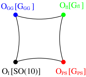
Figure 1: The three SO(10) subgroups at the corresponding fixpoints of the orbifold $T^{2}/(Z_{2}^{I}\times Z_{2}^{PS}\times Z_{2}^{GG})$ .

Compared to [23] we have added an additional pair of bulk 16-plets, $\phi$ and $\phi^{c}$ together with two 10-plets, $H_{5}$ and $H_{6}$, to cancel bulk anomalies. This is still compatible with the embedding in $E_{8}$, and it corresponds to the largest number of bulk fields consistent with the cancellation of anomalies. Note that both the irreducible and reducible 6d gauge anomalies vanish.

The parities of $H_{5}$, $H_{6}$ and $\phi$ are listed in table 1. $\phi^{c}$ has the same parities as $\phi$. The corresponding zero modes are

$$L=\left(\begin{array}[]{l}\nu_{4}\\ e_{4}\end{array}\right)\;,\quad L^{c}=\left(\begin{array}[]{l}\nu^{c}_{4}\\ e^{c}_{4}\end{array}\right)\;,\quad G^{c}_{5}=d^{c}_{4}\;,\quad G_{6}=d_{4}\;.$$ (5)

The zero modes of the fields $\Phi$, $\Phi^{c}$, $H_{1}\ldots H_{4}$ are given in [23]. They are the color triplets and singlets $D^{c}$, $N^{c}$, $D$, $N$, $H_{1}^{c}$, $H_{2}$, $G^{c}_{3}$ and $G_{4}$.

$\begin{array}[h]{|c||cc|cc|cc|cc|}\hline\cr\mbox{SO(10)}&\vrule\lx@intercol\hfil\mathbf{10}\hfil\lx@intercol\vrule\lx@intercol\\ \hline\cr G_{PS}&\vrule\lx@intercol\hfil(\mathbf{1},\mathbf{2},\mathbf{2})\hfil\lx@intercol\vrule\lx@intercol&\vrule\lx@intercol\hfil(\mathbf{1},\mathbf{2},\mathbf{2})\hfil\lx@intercol\vrule\lx@intercol&\vrule\lx@intercol\hfil(\mathbf{6},\mathbf{1},\mathbf{1})\hfil\lx@intercol\vrule\lx@intercol&\vrule\lx@intercol\hfil(\mathbf{6},\mathbf{1},\mathbf{1})\hfil\lx@intercol\vrule\lx@intercol\\ \hline\cr G_{GG}&\vrule\lx@intercol\hfil\mathbf{5}^{\ast}{}_{-2}\hfil\lx@intercol\vrule\lx@intercol&\vrule\lx@intercol\hfil\mathbf{5}{}_{+2}\hfil\lx@intercol\vrule\lx@intercol&\vrule\lx@intercol\hfil\mathbf{5}^{\ast}{}_{-2}\hfil\lx@intercol\vrule\lx@intercol&\vrule\lx@intercol\hfil\mathbf{5}{}_{+2}\hfil\lx@intercol\vrule\lx@intercol\\ \hline\cr&\vrule\lx@intercol\hfil H^{c}\hfil\lx@intercol\vrule\lx@intercol&\vrule\lx@intercol\hfil H\hfil\lx@intercol\vrule\lx@intercol&\vrule\lx@intercol\hfil G^{c}\hfil\lx@intercol\vrule\lx@intercol&\vrule\lx@intercol\hfil G\hfil\lx@intercol\vrule\lx@intercol\\ {}\hfil&Z_{2}^{PS}&Z_{2}^{GG}&Z_{2}^{PS}&Z_{2}^{GG}&Z_{2}^{PS}&Z_{2}^{GG}&Z_{2}^{PS}&Z_{2}^{GG}\\ \hline\cr\hline\cr H_{5}&-&+&-&-&+&+&+&-\\ \hline\cr\hline\cr H_{6}&-&-&-&+&+&-&+&+\\ \hline\cr\end{array}$

$\begin{array}[h]{|c||cc|cc|cc|cc|}\hline\cr\mbox{SO(10)}&\vrule\lx@intercol\hfil\mathbf{16}\hfil\lx@intercol\vrule\lx@intercol\\ \hline\cr G_{PS}&\vrule\lx@intercol\hfil(\mathbf{4},\mathbf{2},\mathbf{1})\hfil\lx@intercol\vrule\lx@intercol&\vrule\lx@intercol\hfil(\mathbf{4},\mathbf{2},\mathbf{1})\hfil\lx@intercol\vrule\lx@intercol&\vrule\lx@intercol\hfil(\mathbf{4}^{\ast},\mathbf{1},\mathbf{2})\hfil\lx@intercol\vrule\lx@intercol&\vrule\lx@intercol\hfil(\mathbf{4}^{\ast},\mathbf{1},\mathbf{2})\hfil\lx@intercol\vrule\lx@intercol\\ \hline\cr G_{GG}&\vrule\lx@intercol\hfil\mathbf{10}_{-1}\hfil\lx@intercol\vrule\lx@intercol&\vrule\lx@intercol\hfil\mathbf{5}^{\ast}{}_{+3}\hfil\lx@intercol\vrule\lx@intercol&\vrule\lx@intercol\hfil\mathbf{10}_{-1}\hfil\lx@intercol\vrule\lx@intercol&\vrule\lx@intercol\hfil\mathbf{5}^{\ast}{}_{+3},\mathbf{1}_{-5}\hfil\lx@intercol\vrule\lx@intercol\\ \hline\cr{}\hfil&\vrule\lx@intercol\hfil Q\hfil\lx@intercol\vrule\lx@intercol&\vrule\lx@intercol\hfil L\hfil\lx@intercol\vrule\lx@intercol&\vrule\lx@intercol\hfil U,E\hfil\lx@intercol\vrule\lx@intercol&\vrule\lx@intercol\hfil D^{c},N^{c}\hfil\lx@intercol\vrule\lx@intercol\\ {}\hfil&Z_{2}^{PS}&Z_{2}^{GG}&Z_{2}^{PS}&Z_{2}^{GG}&Z_{2}^{PS}&Z_{2}^{GG}&Z_{2}^{PS}&Z_{2}^{GG}\\ \hline\cr\phi&+&-&+&+&-&-&-&+\\ \hline\cr\end{array}$

Table 1: Parity assignments for the bulk hypermultiplets $H_{5}$, $H_{6}$ and $\phi$.

Fermion masses and mixings are determined by brane superpotentials. The allowed terms are restricted by R-invariance and an additional U(1)${}_{\tilde{X}}$ symmetry [23]. The corresponding charges of the superfields are given in table 2. The fields $H_{1}$, $H_{2}$, $\Phi$ and $\Phi^{c}$, which aquire a vacuum expectation value, have vanishing R-charge. All matter fields have R-charge one. Since $\psi_{i}$ and $\phi$ have the same charges we combine them to the quartet $(\psi_{\alpha})=(\psi_{i},\phi)$, $\alpha=1\ldots 4$. The most general brane superpotential up to quartic terms is then given by

$$W = M^{d}H_{5}H_{6}+M^{l}_{\alpha}\psi_{\alpha}\phi^{c}+M_{12}H_{1}H_{3}+M_{23}H_{2}H_{3}$$ (6)

$$+{1\over 2}h^{(1)}_{\alpha\beta}\psi_{\alpha}\psi_{\beta}H_{1}+{1\over 2}h^{(2)}_{\alpha\beta}\psi_{\alpha}\psi_{\beta}H_{2}+f_{\alpha}\Phi\psi_{\alpha}H_{6}+f_{5}\Phi^{c}\phi^{c}H_{5}$$

$$+f^{D}\Phi^{c}\Phi^{c}H_{3}+f^{G}\Phi\Phi H_{4}+{1\over 2}{h^{N}_{\alpha\beta}\over M_{*}}\psi_{\alpha}\psi_{\beta}\Phi^{c}\Phi^{c}$$

$$+{k_{1}\over M_{*}}H_{1}^{2}H_{5}^{2}+{k_{2}\over M_{*}}H_{1}H_{2}H_{5}^{2}+{k_{3}\over M_{*}}H_{2}^{2}H_{5}^{2}+{k_{4}\over M_{*}}\Phi\Phi^{c}H_{1}H_{3}$$

$$+{k_{5}\over M_{*}}\Phi\Phi^{c}H_{2}H_{3}+{g^{d}_{\alpha}\over M_{*}}\Phi^{c}\psi_{\alpha}H_{5}H_{1}+{g^{u}_{\alpha}\over M_{*}}\Phi^{c}\psi_{\alpha}H_{5}H_{2}+{g^{d}\over M_{*}}\Phi\phi^{c}H_{5}H_{1}$$

$$+{g^{u}\over M_{*}}\Phi\phi^{c}H_{5}H_{2}+{k^{d}_{\alpha}\over M_{*}}\Phi\Phi^{c}\psi_{\alpha}\phi^{c}+{k^{l}_{\alpha}\over M_{*}}\Phi\Phi^{c}\psi_{\alpha}\phi^{c}+{k^{l}\over M_{*}}\Phi\Phi\phi^{c}\phi^{c}\;,$$

where we choose $M_{*}>1/R_{5,6}\sim\Lambda_{GUT}$ to be the cutoff of the 6d theory, and the bulk fields have been properly normalized. All the volume factors due to the 6d fields are absorbed into the unknown couplings and we will not use them to explain the hierarchies. When the bulk fields are replaced by their zero modes only 9 of the 23 terms appearing in the superpotential remain. Although we have written the superpotential in terms of SO(10) multiplets, on the different branes the Yukawa couplings $h^{(1)}$ and $h^{(2)}$ split into $h^{(d)},h^{(e)}$ and $h^{(u)},h^{(D)}$, respectively. Some of these couplings are equal due to GUT relations on the corresponding brane.

$\begin{array}[h]{| c | c c c c c c c c c c c |}\hline\cr{}\hfil&H_{1}&H_{2}&\Phi^{c}&H_{3}&\Phi&H_{4}&\psi_{i}&\phi^{c}&\phi&H_{5}&H_{6}\\ \hline\cr R&0&0&0&2&0&2&1&1&1&1&1\\ \hline\cr\widetilde{X}&-2a&-2a&-a&2a&a&-2a&a&-a&a&2a&-2a\\ \hline\cr\end{array}$

Table 2: Charge assignments for the symmetries U(1)_R and U(1)${}_{\tilde{X}}$.

The main idea to generate fermion mass matrices is now as follows. We consider the case that the three sequential 16-plets are located on the three branes where SO(10) is broken to its three GUT subgroups. As an example, we place $\psi_{1}$ at $O_{GG}$, $\psi_{2}$ at $O_{fl}$ and $\psi_{3}$ at $O_{PS}$. The three ‘families’ are then separated by distances large compared to the cutoff scale $M_{*}$. Hence, they can only have diagonal Yukawa couplings with the bulk Higgs fields. Direct mixings are exponentially suppressed. However, the brane fields can mix with the bulk zero modes for which we expect no suppression. These mixings take place only among left-handed leptons and right-handed down-quarks. This leads to a characteristic pattern of mass matrices which we shall now explore.

If $B-L$ is broken, as discussed in [23], $\langle\Phi^{c}\rangle=\langle\Phi\rangle=v_{N}$, and the bulk zero modes $N^{c}$, $N$, ($D,G^{c}$) and ($D^{c},G$) aquire masses ${\cal O}(v_{N})$. After electroweak symmetry breaking, with $\langle H^{c}_{1}\rangle=v_{1}$, $\langle H_{2}\rangle=v_{2}$, the remaining states have the following mass terms,

$$W = d_{\alpha}m^{d}_{\alpha\beta}d^{c}_{\beta}+e^{c}_{\alpha}m^{e}_{\alpha\beta}e_{\beta}+n^{c}_{\alpha}m^{D}_{\alpha\beta}\nu_{\beta}$$ (7)

$$+u^{c}_{i}m^{u}_{ij}u_{j}+{1\over 2}n^{c}_{i}M_{ij}n^{c}_{j}\;.$$

Here $m^{d}$, $m^{e}$ and $m^{D}$ are $4\times 4$ matrices,

$$m^{d}=\left(\begin{array}[]{cccc}h^{d}_{11}v_{1}&0&0&g_{1}^{d}{v_{N}\over M_{*}}v_{1}\\ 0&h^{d}_{22}v_{1}&0&g_{2}^{d}{v_{N}\over M_{*}}v_{1}\\ 0&0&h^{d}_{33}v_{1}&g_{3}^{d}{v_{N}\over M_{*}}v_{1}\\ f_{1}v_{N}&f_{2}v_{N}&f_{3}v_{N}&M^{d}\end{array}\right)\;,$$ (12)

$$m^{e}=\left(\begin{array}[]{cccc}h^{d}_{11}v_{1}&0&0&h_{14}^{e}v_{1}\\ 0&h^{e}_{22}v_{1}&0&h_{24}^{e}v_{1}\\ 0&0&h^{d}_{33}v_{1}&h_{34}^{e}v_{1}\\ M^{l}_{1}&M^{l}_{2}&M^{l}_{3}&M^{l}_{4}\end{array}\right)\;,$$ (17)

$$m^{D}=\left(\begin{array}[]{cccc}h^{D}_{11}v_{2}&0&0&h_{14}^{D}v_{2}\\ 0&h^{u}_{22}v_{2}&0&h_{24}^{D}v_{2}\\ 0&0&h^{u}_{33}v_{2}&h_{34}^{D}v_{2}\\ M^{l}_{1}&M^{l}_{2}&M^{l}_{3}&M^{l}_{4}\end{array}\right)\;,$$ (22)

whereas $m^{u}$ and $m^{N}$ are diagonal $3\times 3$ matrices,

$$m^{u}=\left(\begin{array}[]{ccc}h^{u}_{11}v_{2}&0&0\\ 0&h^{u}_{22}v_{2}&0\\ 0&0&h^{u}_{33}v_{2}\end{array}\right)\;,\quad m^{N}=\left(\begin{array}[]{ccc}h^{N}_{11}{v_{N}^{2}\over M_{*}}&0&0\\ 0&h^{N}_{22}{v_{N}^{2}\over M_{*}}&0\\ 0&0&h^{N}_{33}{v_{N}^{2}\over M_{*}}\end{array}\right)\;.$$ (29)

In the matrices $m^{d}$, $m^{e}$ and $m^{D}$ we have neglected corrections ${\cal O}(v_{N}/M_{*})$. The diagonal elements satisfy four GUT relations which correspond to the unbroken SU(5), flipped SU(5) and Pati-Salam subgroups of SO(10).

The crucial feature of the matrices $m^{d}$, $m^{e}$ and $m^{D}$ are the mixings between the six brane states and the two bulk states. The first three rows of the matrices are proportional to the electroweak scale. The corresponding Yukawa couplings have to be hierarchical in order to obtain a realistic spectrum of quark and lepton masses. This corresponds to different strengths of the Yukawa couplings at the different fixpoints of the orbifold. The fourth row, proportional to $M^{d}$, $M^{l}$ and $v_{N}$, is of order the unification scale and, we assume, non-hierarchical.

The mass matrices $m^{d}$, $m^{e}$ and $m^{D}$ are of the form

$$m=\left(\begin{array}[]{cccc}\mu_{1}&0&0&\widetilde{\mu}_{1}\\ 0&\mu_{2}&0&\widetilde{\mu}_{2}\\ 0&0&\mu_{3}&\widetilde{\mu}_{3}\\ \widetilde{M}_{1}&\widetilde{M}_{2}&\widetilde{M}_{3}&\widetilde{M}_{4}\end{array}\right)\;,$$ (34)

where $\mu_{i},\widetilde{\mu}_{i}={\cal O}(v_{1,2})$ and $\widetilde{M}_{i}={\cal O}(\Lambda_{GUT})$. To diagonalize the matrix $m$ it is convenient to define a set of four-dimensional unit vectors as follows,

$$(\widetilde{M}_{1},\ldots\widetilde{M}_{4})=\widetilde{M}e_{4}^{T}\;,\quad e^{T}_{\alpha}e_{\beta}=e^{T}_{\alpha\gamma}e_{\beta\gamma}=\delta_{\alpha\beta}\;.$$ (35)

Using the orthogonal matrices ($\alpha,\beta=1\ldots 4$, $i=1\ldots 3$),

$$V_{\alpha\beta}=(e_{\beta})_{\alpha}\;,\quad U_{\alpha\beta}=\delta_{\alpha\beta}-{1\over\widetilde{M}}\delta_{\alpha 4}(e_{4i}\mu_{i}+e_{44}\widetilde{\mu}_{i})\delta_{\beta i}+{\cal O}\left({v^{2}\over\widetilde{M}^{2}}\right)\;,$$ (36)

we can now perform a change of basis which yields for the mass matrix,

$$m^{\prime}=U^{T}mV=\left(\begin{array}[]{cc}\widehat{m}&0\\ 0&\widetilde{M}\end{array}\right)+{\cal O}\left({v^{2}\over\widetilde{M}^{2}}\right)\;,$$ (39)

where the $3\times 3$ matrix $\widehat{m}$ is given by

$$\widehat{m}=\left(\begin{array}[]{c}\mu_{1}\widehat{e}^{T}_{1}+\widetilde{\mu}_{1}\widehat{e}^{T}_{4}\\ \mu_{2}\widehat{e}^{T}_{2}+\widetilde{\mu}_{2}\widehat{e}^{T}_{4}\\ \mu_{3}\widehat{e}^{T}_{3}+\widetilde{\mu}_{3}\widehat{e}^{T}_{4}\end{array}\right)\;.$$ (43)

Here the three-vectors $\widehat{e}_{\alpha}$, $\alpha=1\ldots 4$, are determined by the four-vectors $e_{i}$, $i=1\ldots 3$, with $(\widehat{e}_{\alpha})_{i}=(e_{i})_{\alpha}$. Note that $\widehat{m}$ is composed of three row vectors of hierarchical length, a structure familiar from lopsided fermion mass models.

The hierarchy of the row vectors suggests to perform a further change of basis such that all remaining mixings are small. Three orthogonal three-vectors $\overline{e}_{i}$, $\overline{e}^{T}_{i}\overline{e}_{j}=\overline{e}_{ik}\overline{e}_{jk}=\delta_{ij}$, can be defined by writing the matrix $\widehat{m}$ in the following form

$$\widehat{m}=\left(\begin{array}[]{l}\overline{\mu}_{1}(\gamma\overline{e}^{T}_{1}+\overline{e}^{T}_{2}+\beta\overline{e}^{T}_{3})\\ \overline{\mu}_{2}(\overline{e}^{T}_{2}+\alpha\overline{e}^{T}_{3})\\ \overline{\mu}_{3}\overline{e}^{T}_{3}\end{array}\right)\;.$$ (47)

The parameters $\overline{\mu}_{i}$ are ${\cal O}(\mu_{i},\widetilde{\mu}_{i})$ and therefore again hierarchical. With respect to this new basis the matrix $m$ has triangular form,

$$\overline{m}=\left(\begin{array}[]{lll}\overline{\mu}_{1}\gamma&\overline{\mu}_{1}&\overline{\mu}_{1}\beta\\ 0&\overline{\mu}_{2}&\overline{\mu}_{2}\alpha\\ 0&0&\overline{\mu}_{3}\end{array}\right)\;.$$ (51)

For our discussion of mass eigenvalues and mixing angles we shall need the two matrices $mm^{T}$ and $m^{T}m$, which in the basis $\overline{e}_{i}$ are both hierarchical,

$$mm^{T}=\left(\begin{array}[]{lll}\overline{\mu}_{1}^{2}(1+\beta^{2}+\gamma^{2})&\overline{\mu}_{1}\overline{\mu}_{2}(1+\alpha\beta)&\overline{\mu}_{1}\overline{\mu}_{3}\beta\\ \overline{\mu}_{1}\overline{\mu}_{2}(1+\alpha\beta)&\overline{\mu}_{2}^{2}(1+\alpha^{2})&\overline{\mu}_{2}\overline{\mu}_{3}\alpha\\ \overline{\mu}_{1}\overline{\mu}_{3}\beta&\overline{\mu}_{2}\overline{\mu}_{3}\alpha&\overline{\mu}_{3}^{2}\end{array}\right)\;,$$ (55)

$$m^{T}m=\left(\begin{array}[]{lll}\overline{\mu}_{1}^{2}\gamma^{2}&\overline{\mu}_{1}^{2}\gamma&\overline{\mu}_{1}^{2}\beta\gamma\\ \overline{\mu}_{1}^{2}\gamma&\overline{\mu}_{2}^{2}+\overline{\mu}_{1}^{2}&\overline{\mu}_{2}^{2}\alpha+\overline{\mu}_{1}^{2}\beta\\ \overline{\mu}_{1}^{2}\beta\gamma&\overline{\mu}_{2}^{2}\alpha+\overline{\mu}_{1}^{2}\beta&\overline{\mu}_{3}^{2}+\overline{\mu}_{2}^{2}\alpha^{2}+\overline{\mu}_{1}^{2}\beta^{2}\end{array}\right)\;.$$ (59)

Consider now the up-quark mass matrix. We concentrate on the case of large $\tan{\beta}=v_{2}/v_{1}\simeq 50$, such that $h^{d}_{33}\simeq h^{u}_{33}$. The diagonal elements of the mass matrices (12), (17), (22) and (29) are partially connected by the GUT relations which hold on the different branes. For simplicity, we therefore assume universally,

$$\mu_{1}:\mu_{2}:\mu_{3}\sim m_{u}:m_{c}:m_{t}\;.$$ (60)

It is well known that the hierarchy of down-quark and charged lepton masses is substantially smaller than the up-quark mass hierarchy. Given the scaling (60) of the diagonal elements and the structure of $m^{d}$ and $m^{e}$ this implies that the down-quark and charged lepton mass matrices must be dominated by the off-diagonal elements. Hence, we assume again universally,

$$\mu_{1}\ll\overline{\mu}_{1}\sim\widetilde{\mu}_{1}\;,\quad\mu_{2}\ll\overline{\mu}_{2}\sim\widetilde{\mu}_{2}\;,\quad\mu_{3}\sim\overline{\mu}_{3}\;.$$ (61)

The parameters $\overline{\mu}_{1,2}$ of the matrix $\overline{m}$ are then dominated by the mixing terms $\widetilde{\mu}_{1,2}$, i.e. $\overline{\mu}_{1,2}\sim\widetilde{\mu}_{1,2}$.

Since the up-quark matrix $m^{u}$ is diagonal the CKM quark mixing matrix is given by the matrix $V$ which diagonalizes $m^{d}m^{dT}$. From eq. (55) one reads off for the two larger masses

$$m_{b}\simeq\overline{\mu}_{3}\;,\quad m_{s}\simeq\widetilde{\mu}_{2}\;,$$ (62)

and for the mixing angles

$$V_{us}=\Theta_{c}\sim{\widetilde{\mu}_{1}\over\widetilde{\mu}_{2}}\;,\quad V_{cb}\sim{\widetilde{\mu}_{2}\over\widetilde{\mu}_{3}}\;,\quad V_{ub}\sim{\widetilde{\mu}_{1}\over\widetilde{\mu}_{3}}\;.$$ (63)

Using $m_{b}$, $m_{s}$ and $\Theta_{c}\simeq 0.2$ as input one obtains for the two remaining mixing angles

$$V_{cb}\sim{m_{s}\over m_{b}}\simeq 2\times 10^{-2}\;,\quad V_{ub}\sim\Theta_{c}{m_{s}\over m_{b}}\simeq 4\times 10^{-3}\;,$$ (64)

in agreement with analyses of weak decays [24] up to a factor of two, which is beyond the predictivity of our approach.

The smallest eigenvalue vanishes in the limit $\mu_{1},\mu_{2}\rightarrow 0$, since in this case two vectors of the matrix $\widehat{m}$ become parallel, with $\beta=\alpha$ and $\gamma=0$. Choosing, for simplicity, $\mu_{1}/\widetilde{\mu}_{1}<\mu_{2}/\widetilde{\mu}_{2}$, one has for non-zero $\mu_{1},\mu_{2}$,

$$\gamma\sim{\mu_{2}\over\widetilde{\mu}_{2}}\sim{m_{c}m_{b}\over m_{t}m_{s}}\sim 0.1\;.$$ (65)

This relation will also be important in our analysis of the neutrino masses. For the down-quark mass one obtains

$${m_{d}\over m_{s}}\sim{\mu_{2}\over\widetilde{\mu}_{2}}{\widetilde{\mu}_{1}\over\widetilde{\mu}_{2}}\sim\ \Theta_{c}\;{m_{c}m_{b}\over m_{t}m_{s}}\simeq\ 0.03\;,$$ (66)

consistent with data [1].

The charged lepton mass matrix $m^{e}$ is very similar to the down-quark mass matrix. The main difference is that now there are large mixings between the ‘left-handed’ states $e_{i}$. To obtain the contribution of the charged leptons to the leptonic mixing matrix we consider the matrix $m^{eT}m^{e}$ as given in eq. (59) in the basis $\overline{e}_{i}$. For the two large eigenvalues of $m^{e}$ one has $m_{\tau}\sim\overline{\mu}_{3}\sim m_{b}$ and $m_{\mu}\sim\overline{\mu}_{2}\sim m_{s}$. These relations are consistent with data within our accuracy. A potential problem is the smallness of the electron mass, i.e. $m_{e}/m_{\mu}\simeq 0.1\;m_{d}/m_{s}$. The smallest eigenvalue of $m^{e}$ is again given by $m_{e}/m_{\mu}\sim(\mu_{2}\widetilde{\mu}_{1}/\widetilde{\mu}_{2}^{2})$. However, in our model the usual SU(5) relations don’t hold for the second row of the mass matrices. Hence, the electron mass is not determined by down quark masses.

Using the diagonal and off-diagonal elements of the mass matrices as determined from up- and down-quark mass matrices, we can now discuss the implications for neutrino masses. The heavy Majorana neutrinos scale like up-quarks (cf. (29)),

$$M_{3}:M_{2}:M_{1}\sim m_{t}:m_{c}:m_{u}\;.$$ (67)

The light neutrino masses are given by the seesaw relation

$$m_{\nu}=-m^{DT}{1\over M^{N}}m^{D}\;.$$ (68)

The structure of the charged lepton and the Dirac neutrino mass matrices (cf. (17),(22)) is the same. Both matrices lead to large mixings between the ‘left-handed’ states. In order to determine the leptonic mixing matrix we discuss the Dirac neutrino matrix in the basis $\overline{e}_{i}$ where the remaining mixings of the left-handed charged leptons is small by construction (cf. (59)).

The Dirac neutrino mass matrix can be written as (cf. (43)),

$$\widehat{m}^{D}=\left(\begin{array}[]{c}\rho_{1}\widehat{e}^{T}_{1}+\widetilde{\rho}_{1}\widehat{e}^{T}_{4}\\ \rho_{2}\widehat{e}^{T}_{2}+\widetilde{\rho}_{2}\widehat{e}^{T}_{4}\\ \rho_{3}\widehat{e}^{T}_{3}+\widetilde{\rho}_{3}\widehat{e}^{T}_{4}\end{array}\right)\;.$$ (72)

Here the parameters $\rho_{i}$, $\widetilde{\rho}_{i}$ are expected to have the same hierarchy as $\mu_{i}$, $\widetilde{\mu}_{i}$. However, in general these parameters will differ by factors ${\cal O}(1)$ since there the entries of $m^{e}$ and $m^{D}$ arise from different Yukawa couplings in the superpotential. This implies for the matrix $\widehat{m}^{D}$, with respect to the vectors $\overline{e}_{i}$,

$$\widehat{m}^{D}=\left(\begin{array}[]{l}\overline{\rho}_{1}(A\overline{e}^{T}_{1}+D\overline{e}^{T}_{2}+\overline{e}^{T}_{3})\\ \overline{\rho}_{2}(B\overline{e}^{T}_{1}+E\overline{e}^{T}_{2}+\overline{e}^{T}_{3})\\ \overline{\rho}_{3}(C\overline{e}^{T}_{1}+F\overline{e}^{T}_{2}+\overline{e}^{T}_{3})\end{array}\right)\;,$$ (76)

where $\overline{\rho}_{i}\simeq\widetilde{\rho}_{i}$. Hence, with respect to the basis $\overline{\mu}_{i}$ the matrix $\widehat{m}^{D}$ has no longer triangular form,

$$\overline{m}^{D}=\left(\begin{array}[]{lll}A\overline{\rho}_{1}&B\overline{\rho}_{1}&\overline{\rho}_{1}\\ C\overline{\rho}_{2}&D\overline{\rho}_{2}&\overline{\rho}_{2}\\ E\overline{\rho}_{3}&F\overline{\rho}_{3}&\overline{\rho}_{3}\end{array}\right)\;.$$ (80)

Generically, the parameters $A\ldots F$ are all ${\cal O}(1)$. All we know is that for $\mu_{1,2}=\rho_{1,2}=0$ the first two row vectors are parallel, with $A=B=C=0$ and $D=E$. For $\mu_{1,2},\rho_{1,2}\neq 0$ one has analogous to the charged lepton mass matrix (cf. (65)),

$$A,B,C,D-E\sim{\rho_{2}\over\widetilde{\rho}_{2}}\sim{\mu_{2}\over\widetilde{\mu}_{2}}\sim\gamma\sim 0.1\;.$$ (81)

From eqs. (68) and (80) one now obtains for the light neutrino mass matrix,

$$-\overline{m}_{\nu}=\overline{m}^{DT}{1\over M^{N}}\overline{m}^{D}=\hskip 312.9803pt$$ (82)

$$\left(\begin{array}[]{lll}A^{2}{\overline{\rho}_{1}^{2}\over M_{1}}+B^{2}{\overline{\rho}_{2}^{2}\over M_{2}}+C^{2}{\overline{\rho}_{3}^{2}\over M_{3}}&AD{\overline{\rho}_{1}^{2}\over M_{1}}+BE{\overline{\rho}_{2}^{2}\over M_{2}}+CF{\overline{\rho}_{3}^{2}\over M_{3}}&A{\overline{\rho}_{1}^{2}\over M_{1}}+B{\overline{\rho}_{2}^{2}\over M_{2}}+C{\overline{\rho}_{3}^{2}\over M_{3}}\\ AD{\overline{\rho}_{1}^{2}\over M_{1}}+BE{\overline{\rho}_{2}^{2}\over M_{2}}+CF{\overline{\rho}_{3}^{2}\over M_{3}}&D^{2}{\overline{\rho}_{1}^{2}\over M_{1}}+E^{2}{\overline{\rho}_{2}^{2}\over M_{2}}+F^{2}{\overline{\rho}_{3}^{2}\over M_{3}}&D{\overline{\rho}_{1}^{2}\over M_{1}}+E{\overline{\rho}_{2}^{2}\over M_{2}}+F{\overline{\rho}_{3}^{2}\over M_{3}}\\ A{\overline{\rho}_{1}^{2}\over M_{1}}+B{\overline{\rho}_{2}^{2}\over M_{2}}+C{\overline{\rho}_{3}^{2}\over M_{3}}&D{\overline{\rho}_{1}^{2}\over M_{1}}+E{\overline{\rho}_{2}^{2}\over M_{2}}+F{\overline{\rho}_{3}^{2}\over M_{3}}&{\overline{\rho}_{1}^{2}\over M_{1}}+{\overline{\rho}_{2}^{2}\over M_{2}}+{\overline{\rho}_{3}^{2}\over M_{3}}\end{array}\right)\;.$$

Using eq. (81) one immediately sees the order of magnitude of the different entries,

$$\overline{m}_{\nu}\sim\left(\begin{array}[]{lll}\gamma^{2}&\gamma&\gamma\\ \gamma&1&1\\ \gamma&1&1\end{array}\right)m_{3}\;,$$ (89)

where $m_{3}$ is the largest neutrino mass, i.e. $m_{1}\leq m_{2}\leq m_{3}$. It is well known that such a matrix can account for all neutrino data. It has previously been derived based on a U(1) family symmetry [16, 17] and also by requiring a compensation between the Dirac and Majorana neutrino mass hierarchies [25, 26].

Consider now the parameters in the matrix (82). The mass matrices $m^{d}$, $m^{e}$ and $m^{D}$ have the same structure with large off-diagonal entries. For simplicity, we therefore assume for the mass parameters $\overline{\mu}_{i}$ and $\overline{\rho}_{i}$ have a similar hierarchy, approximately given by the down-quark masses, i.e. $\overline{\rho}_{1}:\overline{\rho}_{2}:\overline{\rho}_{3}\sim m_{d}:m_{s}:m_{b}$. One then obtains

$${\overline{\rho}_{2}^{2}\over M_{2}}{M_{3}\over\overline{\rho}_{3}^{2}}\sim{m_{s}^{2}m_{t}\over m_{b}^{2}m_{c}}\sim 0.2\;,\quad{\overline{\rho}_{1}^{2}\over M_{1}}{M_{3}\over\overline{\rho}_{3}^{2}}\sim{m_{d}^{2}m_{t}\over m_{b}^{2}m_{u}}\sim 0.2\;.$$ (90)

This corresponds to the picture of sequential heavy neutrino dominance [27]. It yields large 2-3 mixing, $\sin{2\Theta_{23}}\sim 1$. The largest neutrino mass is $m_{3}\sim m_{t}^{2}/M_{3}$. Identifying $m_{3}$ with $\sqrt{\Delta m_{atm}^{2}}\sim 0.05$ eV one obtains for the heavy Majorana masses $M_{3}\sim 10^{15}$ GeV, $M_{2}\sim 3\times 10^{12}$ GeV and $M_{1}\sim 10^{10}$ GeV. The second neutrino mass is $m_{2}\sim 0.01$ eV, which is consistent with data within our accuracy.

Since the 2-3 determinant is small the matrix (82) can also account for the LMA MSW-solution of the solar neutrino problem [20]. As all neutrino masses are rather close to each other, with unknown coefficients ${\cal O}(1)$, a precise prediction of the mixing angle $\Theta_{12}$ and the smallest neutrino mass is not possible. Generically, one has $\sin{2\Theta_{12}}\sim\gamma m_{3}/m_{2}$ and $m_{1}={\cal O}(\gamma m_{3},m_{2})$. On the other hand, a definitive prediction of the matrix (82) is a rather large 1-3 mixing angle, $\Theta_{13}\sim\gamma\sim 0.1$.

Decays of the lightest right-handed neutrinos may be the origin of the baryon asymmetry of the universe [28]. In addition to the mass $M_{1}\sim 10^{10}$ GeV the relevant quantities are the CP-asymmetry $\varepsilon_{1}$ and the effective neutrino mass $\widetilde{m}=(m^{D\dagger}m^{D})_{11}/M_{1}$. One easily obtains $\varepsilon_{1}\sim 0.1\;M_{1}/M_{3}\sim 10^{-6}$ and $\widetilde{m}_{1}\sim 0.2\;m_{3}$. These are the typical parameters of thermal leptogenesis [29].

Starting from three sequential families located at three different fixpoints of an orbifold, we have shown that the mixing with split bulk multiplets can lead to a characteristic pattern of quark and lepton mass matrices which can account for small quark mixings together with large lepton mixings in the charged current. Correspondingly, the quark mass hierarchies are large whereas the small neutrino mass hierarchy follows from the difference of down-quark and up-quark mass hierarchies. The dynamical origin of the hierarchy of Yukawa couplings at the different branes remains to be understood.

We would like to thank A. Hebecker and D. Wyler for helpful discussions.

References

[1]
H. Fritzsch, Z. Xing, Prog. Part. Nucl. Phys. 45 (2000) 1
[2]
G. G. Ross, in Flavor Physics for the Millenium, World Scientific, New Jersey
2001, ed. J.L. Rosner, p. 775
[3]
T. Asaka, W. Buchmüller, L. Covi, Phys. Lett. B 523 (2001) 199
[4]
L. J. Hall, Y. Nomura, T. Okui, D. R. Smith, Phys. Rev. D 65 (2002) 035008
[5]
L. J. Hall, Y. Nomura, Phys. Rev. D 64 (2001) 055003
[6]
A. Hebecker, J. March-Russell, Nucl. Phys. B 613 (2001) 3
[7]
S. M. Barr, Phys. Rev. D 21 (1980) 1424
[8]
N. Haba, T. Kondo, Y. Shimizu, Phys. Lett. B 531 (2002) 245; Phys. Lett. B 535 (2002) 271
[9]
F. P. Correia, M. G. Schmidt, Z. Tavartkiladze, Nucl. Phys. B 649 (2003) 39
[10]
S. M. Barr, I. Dorsner, Phys. Rev. D 66 (2002) 065013
[11]
Q. Shafi, Z. Tavartkiladze, hep-ph/0303150
[12]
H. D. Kim, S. Raby, hep-ph/0304104
[13]
A. Hebecker, J. March-Russell, Phys. Lett. B 541 (2002) 338
[14]
A. Hebecker, J. March-Russell, T. Yanagida, Phys. Lett. B 552 (2003) 229
[15]
C. D. Froggatt, H. B. Nielsen, Nucl. Phys. B 147 (1979) 277
[16]
J. Sato, T. Yanagida, Phys. Lett. B 430 (1998) 127
[17]
N. Irges, S. Lavignac, P. Ramond, Phys. Rev. D 58 (1998) 035003
[18]
C. H. Albright, K. S. Babu, S. M. Barr, Phys. Rev. Lett. 81 (1998) 1167
[19]
W. Buchmüller, T. Yanagida, Phys. Lett. B 445 (1999) 399
[20]
F. Vissani, JHEP 9811 (1998) 25
[21]
G. Altarelli, F. Feruglio, Phys. Lett. B 451 (1999) 388
[22]
T. Asaka, W. Buchmüller, L. Covi, Nucl. Phys. B 648 (2003) 231
[23]
T. Asaka, W. Buchmüller, L. Covi, Phys. Lett. B 540 (2002) 295
[24]
R. Fleischer, Phys. Rep. 370C (2002) 537
[25]
W. Buchmüller, D. Wyler, Phys. Lett. B 521 (2001) 291
[26]
Z. Xing, Phys. Lett. B 545 (2002) 352
[27]
S. F. King, Nucl. Phys. B 576 (2000) 85
[28]
M. Fukugita, T. Yanagida, Phys. Lett. B 174 (1986) 45
[29]
W. Buchmüller, M. Plümacher, Phys. Lett. B 389 (1996) 73