hep-ph/0304141

IFIC/03-10

Reconstructing Neutrino Properties from Collider Experiments in a Higgs Triplet Neutrino Mass Model

D. Aristizábal Sierra¹, M. Hirsch², J. W. F. Valle² and A. Villanova del Moral²

¹ Departamento de Física, Universidad de Antioquia

A.A. 1226  Medellín,  Colombia

² AHEP Group, Institut de Física Corpuscular – C.S.I.C./Universitat de València

Edificio de Institutos de Paterna, Apartado 22085, E–46071 València, Spain

We extend the minimal supersymmetric standard model with bilinear R-parity violation to include a pair of Higgs triplet superfields. The neutral components of the Higgs triplets develop small vacuum expectation values (VEVs) quadratic in the bilinear R-parity breaking parameters. In this scheme the atmospheric neutrino mass scale arises from bilinear R-parity breaking while for reasonable values of parameters the solar neutrino mass scale is generated from the small Higgs triplet VEVs. We calculate neutrino masses and mixing angles in this model and show how the model can be tested at future colliders. The branching ratios of the doubly charged triplet decays are related to the solar neutrino angle via a simple formula.

1 Introduction

Ever since its proposal as a way to generate neutrino masses, either on its own or in the context of effective seesaw schemes [1], many variants of the triplet model have been considered. In fact the triplet is a common ingredient in the formulation of seesaw schemes with gauged [2, 3, 4], or ungauged B-L symmetry [5, 6]. They are also a characteristic feature in several left-right symmetric models [7], required in order to reduce the extended gauge structure down to the minimal $SU(2)\otimes U(1)$. For studies of the phenomenology of left-right symmetric models, both supersymmetric and non-supersymmetric see ref. [8] and references therein.

Recent experiments, including the recently published first results of KamLAND [9], have confirmed the LMA-MSW oscillation solution to the solar neutrino problem [10]. Together with the earlier discoveries in atmospheric neutrinos [11], one can now be fairly confident that all neutrino flavours mix and that at least two non-zero neutrino masses exist. This impressive progress has brought the quest for an understanding of the smallness of neutrino masses to the center of attention in particle physics.

In the standard model neutrinos are massless. One of the best-known mechanisms to generate small (Majorana) neutrino masses is the seesaw mechanism. Elegant as it may be, the seesaw mechanism is not the only theoretically interesting approach to neutrino masses. More interesting from a phenomenological point of view are models in which the neutrino masses are generated at the electroweak scale. Models of this kind include, for example, variants of the seesaw scheme at the electro-weak scale [12, 13], radiative models of neutrino mass [14, 15] and supersymmetry with R-parity violation [17, 18, 19, 20, 21, 22].

In this work we further explore the triplet approach to neutrino mass, by combining it with the idea of bilinear R-parity violating (BRpV) supersymmetry. The later might arise as the effective description of models with spontaneously broken R-parity [23, 24]. Alternatively, the required smallness of the bilinear R parity violating parameters may result from some suitable family symmetry [25], thus providing a common solution [26] to the so-called mu-problem [27] and the neutrino anomalies.

At the superpotential level lepton number violation resides only in the explicit BRpV terms, but after electro-weak symmetry breaking takes place, this induces a naturally small VEV for the neutral component of the Higgs triplets, suppressed by two powers of the BRpV parameters [18], as emphasized recently by Ernest Ma [28] .

The result is a hybrid scheme for the neutrino masses. An attractive and natural possibility is that the atmospheric mass scale arises from bilinear R-parity breaking, while the solar mass scale is generated by the small Higgs triplet VEVs. The model is theoretically simple, since only tree-level physics is required to explain current neutrino data, and has the advantage of being directly testable in the next generation of colliders.

The presence of Higgs triplets would induce lepton flavor violating decays of muons and taus. A number of low-energy constraints on Higgs triplet couplings have been derived from the non-observation of such processes [29]. Although the model we are considering is different from the standard left-right models, many constraints apply equally well to our case. The most important bounds for our model are from the experimental upper limits on $\mu\to 3e$ and $\mu\to e\gamma$, which can be expressed as [29],

$$h_{e\mu}h_{ee}<3.2\times 10^{-7}\frac{M_{\Delta^{--}_{u}}^{2}}{(\rm 100\hskip 2.84526ptGeV)^{2}}$$ (1)

from $\mu\to 3e$ and

$$h_{e\mu}h_{\mu\mu}<2\times 10^{-6}\frac{M_{\Delta^{--}_{u}}^{2}}{(\rm 100\hskip 2.84526ptGeV)^{2}}$$ (2)

from $\mu\to e\gamma$. Here, $h_{ij}$ are the Yukawa couplings of the triplet to the leptons and $M_{\Delta^{--}_{u}}$ is the triplet mass. Note that these bounds are on products of two couplings. Limits exist [29] on individual Yukawa couplings but are weaker by several orders of magnitude.

This paper is organized as follows. In the next section we will present the model, discussing the Higgs potential as well as the mass matrix describing the neutrino-neutralino sector. In Sec. 3 we will then turn to the phenomenology of the model. Neutrino masses and mixings are calculated, with emphasis on the solar neutrino data. Finally production and decays of the Higgs bosons of the model are discussed. In Sec. 3.2 we point out that there is a relation between various branching ratios of the decay of the doubly charged component of the scalar triplet and the solar angle, which will allow to test the validity of the model in a future accelerator. We will then close with a short summary.

2 Model

2.1 Superpotential and scalar sector

The model to be presented below is the supersymmetric extension of the original triplet model of neutrino mass [1] in which the simplest form of R-parity violation is assumed. The model is defined by the particle content of the Minimal Supersymmetric extension of Standard Model (MSSM) augmented by a pair of Higgs triplet superfields:

$$\widehat{\Delta}_{u}=\left(\begin{array}[]{l}\widehat{\Delta}^{++}_{u}\\ \widehat{\Delta}^{+}_{u}\\ \widehat{\Delta}^{0}_{u}\end{array}\right)\qquad\widehat{\Delta}_{d}=\left(\begin{array}[]{l}\widehat{\Delta}^{0}_{d}\\ \widehat{\Delta}^{-}_{d}\\ \widehat{\Delta}^{--}_{d}\end{array}\right)$$ (3)

with hypercharges $Y=+2$ and $Y=-2$ and lepton number $L=-2$ and $L=+2$ respectively. Note that although only one Higgs triplet superfield is necessary to provide the neutrinos with appropriate masses, two triplets are needed to avoid the triangle gauge anomaly. Apart from the new Higgs triplet superfields, we include R-parity violation in three generations, by adding bilinear lepton number violating superpotential terms [16], [17, 19, 20, 21, 22],  [30, 31]. The superpotential of this model is then given by a sum of three terms,

$$W=W_{MSSM}+W_{BRpV}+W_{\Delta}$$ (4)

where

$$W_{MSSM}=-\mu\widehat{H}_{u}\widehat{H}_{d}+h_{U}^{ij}\widehat{H}_{u}\widehat{Q}_{i}\widehat{u}^{c}_{j}+h_{D}^{ij}\widehat{H}_{d}\widehat{Q}_{i}\widehat{d}^{c}_{j}+h_{E}^{ij}\widehat{H}_{d}\widehat{L}_{i}\widehat{e}^{c}_{j}$$ (5)

is the superpotential of the MSSM,

$$W_{BRpV}=\epsilon_{i}\widehat{L}_{i}\widehat{H}_{u}$$ (6)

is the usual bilinear R-parity violating term, while

$$W_{\Delta}=\mu_{\Delta}\widehat{\Delta}_{u}\widehat{\Delta}_{d}+h_{ij}\widehat{L}_{i}\widehat{L}_{j}\widehat{\Delta}_{u}$$ (7)

includes the terms that determine the interactions and masses of the new Higgs triplet superfields. The Yukawa couplings $h_{U}$, $h_{D}$, $h_{E}$ and $h$ are $3\times 3$ matrices in generation space and $\mu$, $\epsilon_{i}$ ($i=1,\ldots,3$) and $M$ are parameters with units of mass.

The scalar potential along neutral directions is a sum of two terms

$$V=V_{SUSY}+V_{soft}$$ (8)

where

$$\begin{array}[]{ccl}V_{SUSY}&=&\left|\mu_{\Delta}\Delta_{u}^{0}\right|^{2}+\left|h^{ij}\widetilde{\nu}_{i}\widetilde{\nu}_{j}+\mu_{\Delta}\Delta_{d}^{0}\right|^{2}+\left|\mu H_{u}^{0}\right|^{2}+\\ &&\\ &&+\frac{1}{8}(g^{2}+g^{\prime 2})\left(\left|H_{d}^{0}\right|^{2}-\left|H_{u}^{0}\right|^{2}+\sum_{i}\left|\widetilde{\nu}_{i}\right|^{2}+2\left|\Delta_{d}^{0}\right|^{2}-2\left|\Delta_{u}^{0}\right|^{2}\right)^{2}+\\ &&\\ &&+\sum_{i}\left|2h^{ij}\widetilde{\nu}_{j}\Delta_{u}^{0}+H_{u}^{0}\epsilon^{i}\right|^{2}+\left|-\mu H_{d}^{0}+\epsilon^{i}\widetilde{\nu}_{i}\right|^{2}\end{array}$$ (9)

is the neutral part of the supersymmetric scalar potential and

$$\begin{array}[]{ccl}V_{soft}&=&\left[A^{ij}h^{ij}\widetilde{\nu}_{i}\widetilde{\nu}_{j}\Delta_{u}^{0}-B\mu H_{d}^{0}H_{u}^{0}+B^{i}\epsilon^{i}\widetilde{\nu}_{i}H_{u}^{0}+B_{\Delta}\mu_{\Delta}\Delta_{u}^{0}\Delta_{d}^{0}+c.c.\right]+\\ &&\\ &&+M_{L}^{2}\sum_{i}\left|\widetilde{\nu}_{i}\right|^{2}+M_{H_{d}}^{2}\left|H_{d}^{0}\right|^{2}+M_{H_{u}}^{2}\left|H_{u}^{0}\right|^{2}+\\ &&\\ &&+M_{\Delta_{u}}^{2}\left|\Delta_{u}^{0}\right|^{2}+M_{\Delta_{d}}^{2}\left|\Delta_{d}^{0}\right|^{2}\end{array}$$ (10)

is the soft supersymmetry breaking scalar potential, also along neutral directions. The expression in eq. (10) contains terms which are linear in the neutral Higgs bosons $H_{u}^{0}$, $H_{d}^{0}$, $\Delta_{u}^{0}$, $\Delta_{d}^{0}$ and the scalar neutrinos $\widetilde{\nu}_{i}$ ($i=1,\ldots,3$). The presence of bilinear RPV terms in the superpotential leads to non-zero sneutrino vacuum expectation values.

The vacuum expectation values can be determined by minimizing the scalar potential in eq. (8). These stationary conditions of the scalar potential are the so-called tadpole equations:

$$\begin{array}[]{lcl}t_{u}&=&-\mu Bv_{d}+(\mu^{2}+M^{2}_{H_{u}})v_{u}+B^{i}\epsilon^{i}v_{i}+\sqrt{2}\epsilon^{i}h_{ij}v^{j}\langle\Delta^{0}_{u}\rangle+\\ &&\\ &&+\epsilon^{i}\epsilon_{i}v_{u}-v_{u}\mathcal{D}\\ &&\\ t_{d}&=&(\mu^{2}+M^{2}_{H_{d}})v_{d}-\mu(Bv_{u}+\epsilon^{i}v_{i})+v_{d}\mathcal{D}\\ &&\\ t^{i}&=&\epsilon^{i}(-\mu v_{d}+B^{i}v_{u}+\epsilon^{j}v_{j})+M^{2}_{L}v^{i}+\sqrt{2}h^{ij}\epsilon_{j}v_{u}\langle\Delta^{0}_{u}\rangle+\\ &&\\ &&+\sqrt{2}A^{ij}h^{ij}v_{j}\langle\Delta^{0}_{u}\rangle+\sqrt{2}\mu_{\Delta}h^{ij}v_{j}\langle\Delta^{0}_{d}\rangle+h^{ij}v_{j}h^{kl}v_{k}v_{l}+\\ &&\\ &&+2h^{ij}h_{jk}v^{k}\langle\Delta^{0}_{u}\rangle^{2}+v^{i}\mathcal{D}\\ &&\\ t_{\langle\Delta^{0}_{u}\rangle}&=&(\mu_{\Delta}^{2}+M^{2}_{\Delta_{u}})\langle\Delta^{0}_{u}\rangle+v^{i}h_{ij}(2h^{jk}v_{k}\langle\Delta^{0}_{u}\rangle+\sqrt{2}\epsilon^{j}v_{u})+\\ &&\\ &&+\frac{1}{\sqrt{2}}A^{ij}h^{ij}v_{i}v_{j}+B_{\Delta}\mu_{\Delta}\langle\Delta^{0}_{d}\rangle-2\langle\Delta^{0}_{u}\rangle\mathcal{D}\\ &&\\ t_{\langle\Delta^{0}_{d}\rangle}&=&(\mu_{\Delta}^{2}+M^{2}_{\Delta_{d}})\langle\Delta^{0}_{d}\rangle+\frac{1}{\sqrt{2}}\mu_{\Delta}h^{ij}v_{i}v_{j}+B_{\Delta}\mu_{\Delta}\langle\Delta^{0}_{u}\rangle+2\langle\Delta^{0}_{d}\rangle\mathcal{D}\end{array}$$ (11)

where the non-zero vacuum expectation values are defined as

$$v_{u}\equiv\langle H_{u}^{0}\rangle,\quad\quad v_{d}\equiv\langle H_{d}^{0}\rangle,\quad\quad v_{i}\equiv\langle\widetilde{\nu}_{i}\rangle\quad(i=,1\ldots,3)$$ (12)

and

$$\mathcal{D}\equiv\frac{1}{8}(g^{2}+g^{\prime 2})(v^{2}_{d}-v^{2}_{u}+\sum_{i}v^{2}_{i}+2\langle\Delta^{0}_{d}\rangle^{2}-2\langle\Delta^{0}_{u}\rangle^{2})$$ (13)

The basic idea of the model is contained in eqs. (11) and (13) and can be understood with the help of the following consideration. The VEVs of the scalar triplets violate lepton number by two units and, therefore, are expected to be small. If $\langle\Delta^{0}_{u}\rangle,\langle\Delta^{0}_{d}\rangle\ll v_{u},v_{d}$,

$$\mathcal{D}\simeq\mathcal{D}^{\prime}\equiv\frac{1}{8}(g^{2}+g^{\prime 2})(v^{2}_{d}-v^{2}_{u}+\sum_{i}v^{2}_{i})$$ (14)

and one can solve eqs. (11) for $\langle\Delta^{0}_{u}\rangle$ and $\langle\Delta^{0}_{d}\rangle$,

$$\begin{array}[]{lcl}\langle\Delta^{0}_{u}\rangle&\simeq&\frac{1}{\sqrt{2}}h^{ij}\frac{v_{i}v_{j}[-A^{ij}(\mu_{\Delta}^{2}+M^{2}_{\Delta_{d}}+2\mathcal{D}^{\prime})+B_{\Delta}\mu_{\Delta}^{2}]-2v_{i}\epsilon_{j}v_{u}(\mu_{\Delta}^{2}+M^{2}_{\Delta_{d}}+2\mathcal{D}^{\prime})}{(\mu_{\Delta}^{2}+M^{2}_{\Delta_{u}}-2\mathcal{D}^{\prime})(\mu_{\Delta}^{2}+M^{2}_{\Delta_{d}}+2\mathcal{D}^{\prime})-(B_{\Delta}\mu_{\Delta})^{2}}\\ &&\\ \langle\Delta^{0}_{d}\rangle&\simeq&\frac{1}{\sqrt{2}}h^{ij}\frac{v_{i}v_{j}[-A^{ij}B_{\Delta}\mu_{\Delta}+\mu_{\Delta}(\mu_{\Delta}^{2}+M^{2}_{\Delta_{u}}-2\mathcal{D}^{\prime})]-2v_{i}\epsilon_{j}v_{u}B_{\Delta}\mu_{\Delta}}{(\mu_{\Delta}^{2}+M^{2}_{\Delta_{u}}-2\mathcal{D}^{\prime})(\mu_{\Delta}^{2}+M^{2}_{\Delta_{d}}+2\mathcal{D}^{\prime})-(B_{\Delta}\mu_{\Delta})^{2}}\end{array}$$ (15)

The Higgs triplet VEVs are quadratic in the RPV parameters, and thus automatically small as long as $v_{i}\ll v_{d},v_{u}$. The smallness of the $v_{i}$, on the other hand, depends on the relative size of $\epsilon_{i}/\mu$ which we assume to be sufficiently smaller than one. Note also that the presence of neutral scalar lepton VEVs produces a mixing between scalars, higgs bosons and scalar neutrinos [21].

2.2 Neutral Fermion Mixing

The Lagrangian contains the following terms involving two neutral fermions and the neutral scalars (Higgs bosons and scalar neutrinos)

$$\begin{array}[]{ccl}\mathcal{L}&\supset&\mu\widetilde{H}_{d}^{0}\widetilde{H}_{u}^{0}-\epsilon^{i}\nu_{i}\widetilde{H}_{u}^{0}+h^{ij}\nu_{i}\nu_{j}\Delta_{u}^{0}+h^{ij}\nu_{i}\widetilde{\nu}_{j}\widetilde{\Delta}_{u}^{0}-\mu_{\Delta}\widetilde{\Delta}_{u}^{0}\widetilde{\Delta}_{d}^{0}+\\ &&\\ &&+\frac{1}{2}(M_{1}\lambda^{\prime}\lambda^{\prime}+M_{2}\lambda\lambda)+\\ &&\\ &&+\frac{i}{\sqrt{2}}g^{\prime}\lambda^{\prime}(-\widetilde{\nu}^{i*}\nu_{i}-H_{d}^{0*}\widetilde{H}_{d}^{0}+H_{u}^{0*}\widetilde{H}_{u}^{0}+2\Delta_{u}^{0*}\widetilde{\Delta}_{u}^{0}-2\Delta_{d}^{0*}\widetilde{\Delta}_{d}^{0})+\\ &&\\ &&+\frac{i}{\sqrt{2}}g\lambda^{3}(\widetilde{\nu}^{i*}\nu_{i}+H_{d}^{0*}\widetilde{H}_{d}^{0}-H_{u}^{0*}\widetilde{H}_{u}^{0}-2\Delta_{u}^{0*}\widetilde{\Delta}_{u}^{0}+2\Delta_{d}^{0*}\widetilde{\Delta}_{d}^{0})\end{array}$$ (16)

After the electroweak and R-parity symmetries break through non-zero vacuum expectation values for the Higgs boson and sneutrinos, the Lagrangian contains the following mass terms involving nine neutral fermions:

$$\mathcal{L}\supset-\frac{1}{2}(\psi^{0})^{T}\mathbf{M_{N}}(\psi^{0})$$ (17)

where the basis is

$$(\psi^{0})^{T}=(\nu_{1},\nu_{2},\nu_{3},-i\lambda^{\prime},-i\lambda^{3},\widetilde{H}^{0}_{d},\widetilde{H}^{0}_{u},\widetilde{\Delta}^{0}_{d},\widetilde{\Delta}^{0}_{u})$$ (18)

and the neutral fermion mass matrix is a $9\times 9$ matrix of the form:

$$\mathbf{M_{N}}=\left(\begin{array}[]{lll}\mathbf{M_{\nu}}&\mathbf{m}_{\mathbf{BRpV}}&\mathbf{m}_{\mathbf{\nu\Delta}}\\ \\ \mathbf{m}^{T}_{\mathbf{BRpV}}&\mathbf{\mathcal{M}_{\chi^{0}}}&\mathbf{m}_{\mathbf{\chi^{0}\Delta}}\\ \\ \mathbf{m}^{T}_{\mathbf{\nu\Delta}}&\mathbf{m}^{T}_{\mathbf{\chi^{0}\Delta}}&\mathbf{M_{\Delta}}\end{array}\right)$$ (19)

where the symmetric matrix

$$\mathbf{M_{\nu}}=\sqrt{2}\langle\Delta^{0}_{u}\rangle\left(\begin{array}[]{ccc}h_{11}&h_{12}&h_{13}\\ h_{12}&h_{22}&h_{23}\\ h_{13}&h_{23}&h_{33}\end{array}\right)$$ (20)

characterizes the direct contribution to the neutrino mass matrix and

$$\mathbf{\mathcal{M}_{\chi^{0}}}=\left(\begin{array}[]{cccc}M_{1}&0&-\frac{1}{2}g^{\prime}v_{d}&\frac{1}{2}g^{\prime}v_{u}\\ 0&M_{2}&\frac{1}{2}gv_{d}&-\frac{1}{2}gv_{u}\\ -\frac{1}{2}g^{\prime}v_{d}&\frac{1}{2}gv_{d}&0&-\mu\\ \frac{1}{2}g^{\prime}v_{u}&-\frac{1}{2}gv_{u}&-\mu&0\end{array}\right)$$ (21)

denotes the standard MSSM neutralino mass matrix. The matrix $\mathbf{m_{BRpV}}$ is given as

$$\mathbf{m_{BRpV}}=\left(\begin{array}[]{cccc}-\frac{1}{2}g^{\prime}v_{1}&\frac{1}{2}gv_{1}&0&\epsilon_{1}\\ -\frac{1}{2}g^{\prime}v_{2}&\frac{1}{2}gv_{2}&0&\epsilon_{2}\\ -\frac{1}{2}g^{\prime}v_{3}&\frac{1}{2}gv_{3}&0&\epsilon_{3}\end{array}\right)$$ (22)

and characterizes the bilinear R-parity Violation, while

$$\mathbf{m_{\nu\Delta}}=\left(\begin{array}[]{cc}0&\frac{1}{\sqrt{2}}h^{1j}v_{j}\\ 0&\frac{1}{\sqrt{2}}h^{2j}v_{j}\\ 0&\frac{1}{\sqrt{2}}h^{3j}v_{j}\end{array}\right)$$ (23)

is the neutrino-Higgs triplet mixing mass matrix. On the other hand,

$$\mathbf{m_{\chi^{0}\Delta}}=\left(\begin{array}[]{cc}-g^{\prime}\langle\Delta^{0}_{d}\rangle&g^{\prime}\langle\Delta^{0}_{u}\rangle\\ g\langle\Delta^{0}_{d}\rangle&-g\langle\Delta^{0}_{u}\rangle\\ 0&0\\ 0&0\end{array}\right)$$ (24)

is the neutralino-Higgs triplet mixing mass matrix and

$$\mathbf{M_{\Delta}}=\left(\begin{array}[]{cc}0&\mu_{\Delta}\\ \mu_{\Delta}&0\end{array}\right)$$ (25)

is the Higgs triplet mass matrix arising from the first term in eq. (7).

One sees that the mixing between neutral fermions (gauginos, Higgsinos and neutrinos) has a rich structure, with several off-diagonal RPV entries which, as we show next, will induce masses (and mixings) for the neutrinos.

3 Phenomenology

In what follows we will work in an approximation where we neglect the radiatively induced neutrino masses with respect to those induced at the tree level due to the presence of the triplet. We have checked that there is a natural range of parameters in the model where the use of this approximation is justified. For a thorough discussion of loop-induced neutrino masses in BRpV see refs. [31, 30].

3.1 Neutrino masses and mixing angles

One can provide an approximate analytical understanding of the tree level neutrino masses and mixing angles, by using the previous form of $\mathbf{M_{N}}$. This form is especially convenient because the various sub-blocks in eq. (19) can easily have vastly different orders of magnitude and one expects from eq. (15) and eq. (11)

$$\mathbf{M_{\nu}},\mathbf{m_{\nu\Delta}},\mathbf{m_{\chi^{0}\Delta}}\ll\mathbf{m_{BRpV}}\ll\mathbf{{\cal M}_{\chi^{0}}},\mathbf{M_{\Delta}}$$ (26)

if $\epsilon_{i}<\mu$. More technically, in the limit where $\xi_{ij}\ll 1$, where $\xi={\bf m_{BRpV}}\times{\cal M}_{\chi^{0}}^{-1}$ one can write the effective contribution of the BRpV parameters to the ($3\times 3$) neutrino mass matrix as

$$\mathbf{M_{\nu}^{eff}}=\mathbf{M_{\nu}}+\mathbf{M^{eff}_{Bilinear}}$$ (27)

where the contributions from BRpV to the neutrino mass matrix is given by [30]

$$(\mathbf{M^{eff}_{Bilinear}})_{ij}=\frac{M_{1}g^{2}+M_{2}g^{\prime 2}}{4\det(\mathbf{\mathcal{M}_{\chi^{0}}})}\Lambda_{i}\Lambda_{j}$$ (28)

with

$$\Lambda_{i}=\mu v_{i}+\epsilon_{i}v_{d}.$$ (29)

With the observation eq. (26) one can further simplify the eigenvalue problem of eq. (27), by means of a perturbative diagonalization. Consider first eq. (28). As has been discussed several times in the literature [31], this mass matrix is diagonalized by only two angles,

$$\tan\theta_{13}=-\frac{\Lambda_{e}}{(\Lambda_{\mu}^{2}+\Lambda_{\tau}^{2})^{\frac{1}{2}}},$$ (30)

$$\tan\theta_{23}=-\frac{\Lambda_{\mu}}{\Lambda_{\tau}}.$$ (31)

and leads to only one non-zero eigenvalue, given by

$$m_{\nu}^{BRpV}=\frac{M_{1}g^{2}+M_{2}g^{\prime 2}}{4\det(\mathbf{\mathcal{M}_{\chi^{0}}})}|\Lambda|^{2},$$ (32)

where $|\Lambda|^{2}=\sum\Lambda_{i}^{2}$ The remaining angle $\theta_{12}$ is not defined in the bilinear only model at tree-level. The complete diagonalization of eq. (27), $\mathbf{\widehat{M}_{\nu}^{eff}}=\mathbf{R}\cdot\mathbf{M_{\nu}^{eff}}\cdot\mathbf{R}^{T}$, where the matrix of eigenvectors $\mathbf{R}$ can be expressed as a product of three Euler rotations, can therefore be written as,

$$\begin{array}[]{ccl}\mathbf{\widehat{M}_{\nu}^{effective}}&=&\mathbf{R}\cdot\mathbf{M^{eff}_{Bilinear}}\cdot\mathbf{R}^{T}+\mathbf{R}\cdot\mathbf{M_{\nu}}\cdot\mathbf{R}^{T}\\ &=&\mathbf{R_{12}}\cdot\mathbf{M^{\prime eff}_{Bilinear}}\cdot\mathbf{R_{12}}^{T}+\mathbf{R_{12}}\cdot\mathbf{M^{\prime}_{\nu}}\cdot\mathbf{R_{12}}^{T}\end{array}$$ (33)

Since $\mathbf{M^{\prime eff}_{Bilinear}}$ is already diagonal, the solar angle is defined by the entries of $\mathbf{M^{\prime}_{\nu}}$ only,

$$\tan(2\theta_{SOL})\simeq\frac{2(\mathbf{M^{\prime}_{\nu}})_{12}}{(\mathbf{M^{\prime}_{\nu}})_{11}-(\mathbf{M^{\prime}_{\nu}})_{22}}$$ (34)

Note that $\mathbf{M^{\prime}_{\nu}}$ is not exactly diagonal after applying the rotation eq. (34). However if $\mathbf{M^{\prime}_{\nu}}\ll\mathbf{M^{\prime eff}_{Bilinear}}$, this small off-diagonals will change the angles defined in eq. (30) and eq. (31) only by a negligible amount. Using the experimentally measured values of $\tan^{2}\theta_{ATM}\simeq 1$ and $\sin^{2}2\theta_{\textsc{chooz}}\ll 1$ one can finally find a simple formula for the solar angle ($\theta_{12}$) which is approximately given by

$$\tan(2\theta_{SOL})\simeq\frac{-2\sqrt{2}(h_{12}-h_{13})}{-2h_{11}+h_{22}+h_{33}-2h_{23}}\equiv x$$ (35)

From the above discussion one expects that, for reasonable ranges of parameters, atmospheric neutrino physics is determined by the bilinear parameters $\Lambda_{i}$, whereas the solar neutrino mass scale depends mostly on the Yukawa couplings and the triplet mass.

Fig. 1 shows an example of the solar and atmospheric neutrino mass–squared differences as a function of the Yukawa parameter $h$ for a fixed value of the triplet mass $M_{\Delta}=500$ GeV. These results correspond to the following choice of the MSSM parameters, $M_{2}=120$ GeV, $\mu=500\textrm{GeV}$, $\tan\beta=5$, $A=-500\textrm{GeV}$. In order to ensure a) negligible loop corrections due to the bilinear parameters and b) correct neutrino mixing angles we have chosen the BRpV parameters as follows: $\epsilon_{1}=\epsilon_{2}=\epsilon_{3}$ with $\epsilon^{2}=10^{-3}|\vec{\Lambda}|$ and $\Lambda_{\mu}=\Lambda_{\tau}=10\Lambda_{e}$. The absolute value of $|\vec{\Lambda}|$ can be estimated by $|\vec{\Lambda}|^{2}=\frac{\sqrt{\Delta m^{2}_{\textsc{atm}}}}{\left(\frac{M_{1}g^{2}+M_{2}g^{\prime 2}}{4\det{\mathcal{M}_{\chi^{0}}}}\right)}$. In the numerical estimate we took the best fit $\Delta m^{2}_{\textsc{atm}}=2.5\times 10^{-3}\textrm{eV}^{2}$ given in [10].

One sees that, for the hierarchical spectra produced by the model, $m_{\nu_{2}}\simeq\sqrt{\Delta m^{2}_{\textsc{sol}}}$ scales approximately like $m_{\nu_{2}}\sim h^{2}$. This is expected from eq. (20) and eq. (15). For values of $h\simeq{\cal O}(0.1)$, $\Delta m^{2}_{\textsc{sol}}$ is in the range of the LMA-MSW solution of the solar neutrino problem. For larger values of $M_{\Delta}$ the resulting $m_{\nu_{2}}$ gets smaller approximately like $1/M_{\Delta}$. From Fig. 1 one also sees that for large values of the Yukawas both solar and atmospheric masses are generated by the triplet.

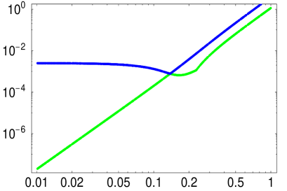
$\Delta m^{2}_{\textsc{atm}},\;\Delta m^{2}_{\textsc{sol}}\;[eV^{2}]$

$h$                                            $\Delta m^{2}_{\textsc{atm}}$
                                                    $\Delta m^{2}_{\textsc{sol}}$

Figure 1: Typical behavior of $\Delta m^{2}_{\textsc{atm}}$ and $\Delta m^{2}_{\textsc{sol}}$ vs. the total Higgs triplet Yukawa coupling $h$, for the arbitrary choice of $h_{11}=h_{23}=h/14$, $\,h_{22}=h_{33}=h_{13}=2\,h/7$, $\,h_{12}=0$. The triplet mass has been fixed at $M_{\Delta}=500$ GeV and the MSSM and BRpV choices are specified in the text.

To check to which degree the simplified results for the solar angle discussed above hold we have constructed a set of randomly chosen sample points and diagonalized the neutrino-neutralino mass matrix numerically. Points were chosen as follows. For the MSSM parameters we scan randomly over the following ranges: $m_{0}$ in the interval [$0,1$] TeV, $M_{2}$ and $\mu$ from [$0,500$] GeV, with both signs for $\mu$, and $\tan\beta$ in [$2,15$]. The resulting SUSY spectra were checked to obey existing lower limits on sparticle searches. For the BRpV parameters consistency with the atmospheric neutrino data requires $|\Lambda|$ in the range [$0.05,0.15$] GeV², $\Lambda_{\mu}\simeq\Lambda_{\tau}$ and $\Lambda_{e}\leq 0.3\sqrt{\Lambda_{\mu}^{2}+\Lambda_{\tau}^{2}}$.

To reduce the number of free parameters we assume $M_{T}\equiv\mu_{\Delta}=M_{\Delta_{u}}=M_{\Delta_{d}}=B_{\Delta}$. We then have calculated neutrino masses and mixing angles for several values of the triplet mass, scanning randomly over the Yukawa couplings with the over-restrictive constraint $h\equiv\sum_{i\leq j}h_{ij}\leq 1$.

$\tan^{2}\theta_{\textsc{sol}}$

$y$

Figure 2: Solar neutrino mixing angle vs. the ratio of triplet Yukawa couplings $y\equiv\tan^{2}\left(\frac{\arctan(x)}{2}\right)$, where $x\equiv\frac{-2\sqrt{2}(h_{12}-h_{13})}{-2h_{11}+h_{22}+h_{33}-2h_{23}}$ and $M_{T}=500$ GeV.

Fig. 2 shows the numerically calculated $\tan^{2}\theta_{\textsc{sol}}$ versus our simple formula eq. (35). Clearly, for the region of interest the simple approximation works surprisingly well. Note, that deviations between the exact and the approximate results mainly occur in the region of parameter space where $h_{12}\simeq h_{13}$.

3.2 Implications for Accelerators

Since in our model R-parity is violated, the lightest supersymmetric particle will decay. As has been shown in [33, 34, 35], bilinear parameters can then be traced through the study of LSP decays. This feature will also remain to be true in the current model. We will not repeat the discussion and instead concentrate on the Higgs triplet in the following.

One of the characteristic features of the triplet model of neutrino mass is the presence of doubly charged Higgs bosons $\Delta^{--}_{u}$. Here we consider its production cross section at an $e^{-}e^{-}$ linear collider at 500 GeV center of mass energy[36]. In Fig. 3 we present the s-channel production cross section for a doubly charged Higgs boson as a function of its mass. For typical expected luminosities of 500 inverse femtobarns per year [32] this implies a very large number of events, half a million or more, for a 500 GeV mass, depending on the leptonic branching ratio in question.

$\sigma(\sqrt{s}=M_{\Delta_{u}})$[fb]

$M_{\Delta_{u}}$[GeV]

Figure 3: Cross section for the production of the Higgs triplet at center of mass energy equal to the triplet mass, $\sigma(\sqrt{s}=M_{\Delta_{u}})$, vs. the triplet mass. The four lines corresponds to a branching ratio (from top to bottom) of $BR(e^{-}e^{-}\to\Delta_{u}^{--})=10^{-1}$, $10^{-2}$, $10^{-3}$ and $10^{-4}$.

The next issue are the decays of such Higgs bosons. Here we come to the most remarkable feature of the present model, namely that the decays of the doubly charged Higgs bosons are a perfect tracer of the neutrino mixing angles. The situation here is similar to that found in the simplest bilinear R-parity model of neutrino mass considered in refs. [33, 34, 35] (and references therein). There it was found that, depending on the nature of the lightest supersymmetric particle, its decays patterns reflect in a simple way either the solar or the atmospheric mixing angles. Here we have in addition that the doubly charged Higgs bosons decay according to the solar mixing angle.

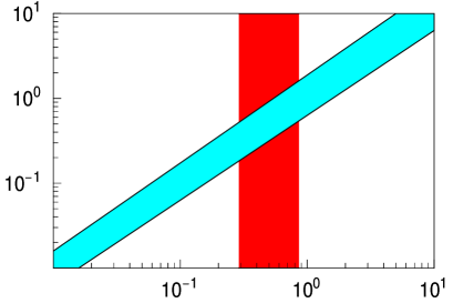
$y_{exp}$

$\tan^{2}(\theta_{\textsc{sol}})$

Figure 4: Ratio of doubly charged Higgs boson decay branching ratios indicated by the variable $y_{exp}$ of eqs. (36) and (37) vs. the solar neutrino mixing angle. The vertical band indicates currently favored values (see ref. [10] and references therein).

In Fig. 4 we give the ratio of doubly charged Higgs boson decay branching ratios versus the solar neutrino mixing angle. The ratio of doubly charged Higgs boson decay branching ratios we consider is specified by the variable

$$y_{exp}\equiv\tan^{2}\left(\frac{\arctan(x_{exp})}{2}\right)$$ (36)

where

$$x_{exp}\equiv\frac{-2\sqrt{2}(\sqrt{BR_{12}}-\sqrt{BR_{13}})}{-2\sqrt{2BR_{11}}+\sqrt{2BR_{22}}+\sqrt{2BR_{33}}-2\sqrt{BR_{23}}}$$ (37)

with $BR_{ij}$ denoting the measured branching ratio for the process ($\Delta_{u}^{--}\to l_{i}^{-}l_{j}^{-}$). Note that the band in the plot includes an assumed $10\%$ uncertainty in the measured branching ratios. The triplet mass has been fixed at $M_{\Delta_{u}}=500$ GeV. As can be seen from the figure, there is a very strong correlation between the pattern of Higgs decays and the mixing angle involved in the solar neutrino problem. The range permitted by current solar and reactor neutrino data [10] is indicated by the vertical band in Fig. 4. This correlation can be used as the basis for a reconstruction of neutrino angles using only accelerator experiments. This provides a cross-check of the determination provided by laboratory and underground searches for neutrino oscillations.

4 Summary and Conclusions

We have extended the minimal supersymmetric standard model by adding bilinear R-parity violation as well as a pair of Higgs triplet superfields. The neutral components of the Higgs triplets develop small induced vacuum expectation values (VEVs) which depend quadratically upon the bilinear R-parity breaking parameters. In this scheme, for reasonable values of parameters, the atmospheric neutrino mass scale arises from bilinear R-parity breaking while the solar neutrino mass scale is generated from the small Higgs triplet VEVs. We have calculated the pattern of neutrino masses and mixing angles in this model and shown how the model can be tested at future colliders. The branching ratios of the doubly charged triplet decays are related to the solar neutrino angle via a simple formula. Similarly the atmospheric mixing can be inferred from the neutralino decay branching ratios, as discussed in ref. [35]. This will allow a full reconstruction of neutrino angles purely from high energy accelerator experiments. The model will be tested in a straightforward way should a high luminosity and center-of-mass energy linear collider ever be built.

References

• [1] J. Schechter and J. W. F. Valle, Phys. Rev. D22, 2227 (1980).
• [2] M. Gell-Mann, P. Ramond and R. Slansky, Print-80-0576 (CERN).
• [3] T. Yanagida, ed. Sawada and Sugamoto (KEK, 1979).
• [4] R. N. Mohapatra and G. Senjanovic, Phys. Rev. D23, 165 (1981).
• [5] Y. Chikashige, R. N. Mohapatra and R. D. Peccei, Phys. Lett. B98, 265 (1981).
• [6] J. Schechter and J. W. F. Valle, Phys. Rev. D25, 774 (1982).
• [7] J. C. Pati and A. Salam, Phys. Rev. D10, 275 (1974).
• [8] N. G. Deshpande, J. F. Gunion, B. Kayser and F. I. Olness, Phys. Rev. D44, 837 (1991). For a recent paper on Higgs triplet and accelerator phenomenology see, for example: E.J. Chun, K.Y. Lee and S.C. Park, hep-ph/0304069
• [9] KamLAND, K. Eguchi et al., Phys. Rev. Lett. 90, 021802 (2003), [hep-ex/0212021].
• [10] For an updated global fit of solar, atmospheric and reactor neutrino data including the recent KamLAND data see, for example, the archive version of M. Maltoni, T. Schwetz, M. A. Tortola and J. W. Valle, Phys. Rev. D 67 (2003) 013011 [arXiv:hep-ph/0207227]; M. Maltoni, T. Schwetz and J. W. Valle, arXiv:hep-ph/0212129 (Phys. Rev. D, in press). For a review see S. Pakvasa and J. W. F. Valle, hep-ph/0301061.
• [11] Super-Kamiokande, Y. Fukuda et al., Phys. Rev. Lett. 81, 1562 (1998), [hep-ex/9807003].
• [12] R. N. Mohapatra and J. W. F. Valle, Phys. Rev. D34, 1642 (1986).
• [13] M. C. Gonzalez-Garcia and J. W. F. Valle, Phys. Lett. B216, 360 (1989).
• [14] A. Zee, Phys. Lett. B93, 389 (1980).
• [15] K. S. Babu, Phys. Lett. B203, 132 (1988).
• [16] M. A. Diaz, J. C. Romao and J. W. F. Valle, Nucl. Phys. B524, 23 (1998), [hep-ph/9706315].
• [17] L. J. Hall and M. Suzuki, Nucl. Phys. B231, 419 (1984). G. G. Ross and J. W. F. Valle, Phys. Lett. B151, 375 (1985). J. R. Ellis, G. Gelmini, C. Jarlskog, G. G. Ross and J. W. F. Valle, Phys. Lett. B150, 142 (1985).
• [18] A. Santamaria and J. W. F. Valle, Phys. Rev. D39, 1780 (1989). Phys. Rev. Lett. 60, 397 (1988). Phys. Lett. B195, 423 (1987).
• [19] T. Banks, Y. Grossman, E. Nardi and Y. Nir, Phys. Rev. D52, 5319 (1995), [hep-ph/9505248]. R. Hempfling, Nucl. Phys. B478, 3 (1996), [hep-ph/9511288]. B. de Carlos and P. L. White, Phys. Rev. D54, 3427 (1996), [hep-ph/9602381]. A. S. Joshipura and M. Nowakowski, Phys. Rev. D51, 2421 (1995), [hep-ph/9408224]. G. Bhattacharyya, D. Choudhury and K. Sridhar, Phys. Lett. B349, 118 (1995), [hep-ph/9412259]. A. Y. Smirnov and F. Vissani, Nucl. Phys. B460, 37 (1996), [hep-ph/9506416]. M. Nowakowski and A. Pilaftsis, Nucl. Phys. B461, 19 (1996), [hep-ph/9508271]. S. Roy and B. Mukhopadhyaya, Phys. Rev. D55, 7020 (1997), [hep-ph/9612447].
• [20] D. E. Kaplan and A. E. Nelson, JHEP 01, 033 (2000), [hep-ph/9901254]. C.-H. Chang and T.-F. Feng, Eur. Phys. J. C12, 137 (2000), [hep-ph/9901260]. M. Frank, Phys. Rev. D62, 015006 (2000). F. Takayama and M. Yamaguchi, Phys. Lett. B476, 116 (2000), [hep-ph/9910320].
• [21] A. G. Akeroyd, M. A. Diaz, J. Ferrandis, M. A. Garcia-Jareno and J. W. F. Valle, Nucl. Phys. B529, 3 (1998), [hep-ph/9707395]. A. G. Akeroyd, M. A. Diaz and J. W. F. Valle, Phys. Lett. B441, 224 (1998), [hep-ph/9806382]. M. A. Diaz, E. Torrente-Lujan and J. W. F. Valle, Nucl. Phys. B551, 78 (1999), [hep-ph/9808412]. M. A. Diaz, D. A. Restrepo and J. W. F. Valle, Nucl. Phys. B583, 182 (2000), [hep-ph/9908286]. M. A. Diaz, J. Ferrandis and J. W. F. Valle, Nucl. Phys. B573, 75 (2000), [hep-ph/9909212]. J. Ferrandis, Phys. Rev. D60, 095012 (1999), [hep-ph/9810371]. F. De Campos, M. A. Diaz, O. J. P. Eboli, M. B. Magro and P. G. Mercadante, Nucl. Phys. B623, 47 (2002), [hep-ph/0110049].
• [22] K. Choi, E. J. Chun and K. Hwang, Phys. Lett. B488, 145 (2000), [hep-ph/0005262]. K.-m. Cheung and O. C. W. Kong, Phys. Rev. D64, 095007 (2001), [hep-ph/0101347]. T.-F. Feng and X.-Q. Li, Phys. Rev. D63, 073006 (2001), [hep-ph/0012300]. E. J. Chun and S. K. Kang, Phys. Rev. D61, 075012 (2000), [hep-ph/9909429]. E. J. Chun, D.-W. Jung and J. D. Park, hep-ph/0211310. F. Borzumati and J. S. Lee, Phys. Rev. D66, 115012 (2002), [hep-ph/0207184]. E. J. Chun and J. S. Lee, Phys. Rev. D60, 075006 (1999), [hep-ph/9811201]. A. Abada, S. Davidson and M. Losada, Phys. Rev. D65, 075010 (2002), [hep-ph/0111332].
• [23] A. Masiero and J. W. F. Valle, Phys. Lett. B251, 273 (1990).
• [24] DELPHI, P. Abreu et al., Phys. Lett. B502, 24 (2001), [hep-ex/0102045].
• [25] J. M. Mira, E. Nardi, D. A. Restrepo and J. W. F. Valle, Phys. Lett. B492, 81 (2000), [hep-ph/0007266].
• [26] H.-P. Nilles and N. Polonsky, Nucl. Phys. B484, 33 (1997), [hep-ph/9606388].
• [27] G. F. Giudice and A. Masiero, Phys. Lett. B206, 480 (1988).
• [28] E. Ma, Mod. Phys. Lett. A17, 1259 (2002), [hep-ph/0205025].
• [29] M. L. Swartz, Phys. Rev. D40, 1521 (1989). K. Huitu, J. Maalampi, A. Pietila, M. Raidal and R. Vuopionpera, arXiv:hep-ph/9701386. G. Barenboim, K. Huitu, J. Maalampi and M. Raidal, Phys. Lett. B 394 (1997) 132 [arXiv:hep-ph/9611362]. F. Cuypers and S. Davidson, Eur. Phys. J. C 2 (1998) 503 [arXiv:hep-ph/9609487].
• [30] M. Hirsch, M. A. Diaz, W. Porod, J. C. Romao and J. W. F. Valle, Phys. Rev. D62, 113008 (2000), [hep-ph/0004115].
• [31] M. A. Diaz, M. Hirsch, W. Porod, J. C. Romao and J. W. F. Valle, hep-ph/0302021.
• [32] B. Badelek et al. [ECFA/DESY Photon Collider Working Group Collaboration], “TESLA Technical Design Report, Part VI, Chapter 1: Photon collider at TESLA,” arXiv:hep-ex/0108012.
• [33] M. Hirsch, W. Porod, J. C. Romao and J. W. Valle, Phys. Rev. D 66, 095006 (2002) [arXiv:hep-ph/0207334].
• [34] D. Restrepo, W. Porod and J. W. Valle, Phys. Rev. D 64, 055011 (2001) [arXiv:hep-ph/0104040].
• [35] W. Porod, M. Hirsch, J. Romao and J. W. Valle, Phys. Rev. D 63, 115004 (2001) [arXiv:hep-ph/0011248].
• [36] J. F. Gunion, Int. J. Mod. Phys. A 13 (1998) 2277 [arXiv:hep-ph/9803222]. ibid A 11 (1996) 1551 [arXiv:hep-ph/9510350].