KAIST-TH2003/03
UCB-PTH-03/08
 
 
Successful Modular Cosmology

Abstract

We present a modular cosmology scenario where the difficulties encountered in conventional modular cosmology are solved in a self-consistent manner, with definite predictions to be tested by observation. Notably, the difficulty of the dilaton finding its way to a precarious weak coupling minimum is made irrelevant by having eternal modular inflation at the vacuum supersymmetry breaking scale after the dilaton is stabilised. Neither this eternal inflation nor the subsequent non-slow-roll modular inflation destabilise the dilaton from its precarious minimum due to the low energy scale of the inflation and consequent small back reaction on the dilaton potential. The observed flat CMB spectrum is obtained from fluctuations in the angular component of a modulus near a symmetric point, which are hugely magnified by the roll down of the modulus to Planckian values, allowing them to dominate the final curvature perturbation. We also give precise calculations of the spectral index and its running.

PACS: 98.80.Cq

1 Introduction

Early Universe cosmology offers one of the few opportunities to test the framework of particle theory phenomenology at high energy scales, in particular string/M-theory phenomenology. Indeed, moduli are generic in string/M-theory, and much attention has been drawn to cosmology where moduli play important roles in the early Universe [1]. This has been referred to as ‘modular cosmology’. Unfortunately, despite many attempts to find viable cosmology scenarios associated with moduli, they turned out to give us cosmological obstacles [2, 3, 4] rather than attractive features.

Our main goal in this paper is to present a successful modular cosmology scenario where those difficulties due to moduli can be solved in a simple and self-consistent manner. Furthermore, this scenario gives definite predictions to be tested by forthcoming observations.

The paper is structured as follows.

Section 2.1 gives our motivation for the investigation of modular cosmology and discusses the cosmological difficulties involving moduli. Section 2.2 outlines how those difficulties are overcome in our proposed scenario.

Section 3.1 discusses eternal inflation [5] at the vacuum supersymmetry breaking scale, which is crucial in solving the dilaton stabilization problem. Section 3.2 is devoted to the non-slow-roll modular inflation which naturally follows the eternal inflation, and whose low energy scale is crucial not to disturb the dilaton potential.

Section 4 gives a detailed analysis of the density perturbations produced in our modular cosmology, starting in Section 4.1 with a brief review of the $\delta N$ formalism [6] necessary to analyse the contributions of the fluctuations in the multiple light degrees of freedom to the final curvature perturbation.

Section 5 briefly discusses thermal inflation’s solution of the Polonyi/moduli problem.

Section 6 gives our conclusions.

Facing the fact that our knowledge of string/M-theory is still too limited to fully describe the moduli dynamics in early Universe, we keep our discussion on string/M-theory aspects fairly general with emphasis on cosmological consequences to be compared with data. We hope our scenario can open up new possibilities in model building of modular cosmology which can be tested by observations.

2 Motivation

2.1 Difficulties in Modular Cosmology

Moduli are generic predictions of string/M theory, but pose major cosmological problems.

The stabilization of the dilaton is a serious problem in both particle physics and cosmology. In a typical setup, one simply cannot find a minimum in the weak coupling regime [3]. More complicated models, such as the racetrack scheme [7], can realize a minimum at weak coupling with a moderate amount of fine-tuning (which is easily anthropically justified if there is no better solution). However, even if there exists such a minimum, it has only a shallow barrier separating it from the runaway part of the dilaton’s potential, and a steeply rising potential on the other side. Thus any typical cosmological history would lead the dilaton to over-shoot the desired weak coupling minimum and roll off along the runaway potential towards zero coupling [4].

Another serious cosmological problem is the cosmological moduli problem. Many moduli are expected to have Planckian vacuum expectation values relative to any symmetric points where they couple to other fields, giving them gravitationally suppressed couplings to other light fields. Shifting of their minima due to supersymmetry breaking in the early universe causes them to dominate the energy density of Universe, and they survive until or beyond nucleosynthesis destroying its successful predictions [2].

Thus, the ubiquitous moduli predicted by string/M-theory have given us a cosmological headache rather than helping us build a desirable cosmology scenario. It is therefore worth while to seek realistic modular cosmology scenarios where those serious cosmological problems are solved without fine-tuning in a self-consistent manner, and we address such a possibility in this paper.

2.2 Successful Modular Cosmology

Let us outline the key ingredients in our successful modular cosmology scenario.

One of the main features in our scenario is eternal modular inflation at the vacuum supersymmetry breaking scale. This is important because the infinite expansion of eternal inflation compensates for any finite unnaturalness in initial conditions. In particular, it can compensate for the extreme fine tuning of initial conditions required for the dilaton to find its way into a precarious weak coupling minimum. The importance of the low energy scale is that it ensures that the dilaton does not get disturbed from its minimum after the eternal inflation ends locally. If one had eternal inflation at a higher energy scale than the scale of vacuum supersymmetry breaking, the backreaction on the dilaton’s potential would dominate over the dilaton’s vacuum potential, and one could never expect the dilaton to find its way into its desired weak coupling minimum after the eternal inflation ends. Moreover, if eternal inflation occurs at a higher energy scale than the vacuum moduli potential, the moduli will roll down to possibly several vacua including run-away vacua, also leading to domain wall problems.

Of course, we do not mean that all of eternal inflation takes place at this low energy scale, just that the last eternal inflation (from our local point of view) occurred at that low energy scale. The full picture of eternal inflation would be of eternal inflation at the various discrete points in field space, from the Planck density down, corresponding to suitable false vacua or maxima with rare, but finitely rare, transitions between these points, and of course continually generating non-eternally inflating regions like our own [8, 9, 10].

Since the last eternal inflation occurred at the vacuum supersymmetry breaking scale, the inflation that produced the observed approximately scale-invariant density perturbations must have occurred at that scale or below. Such inflation emerges naturally as the modulus rolls away from its eternally inflating maximum. The scale-invariance is not automatic but can arise naturally when proper account of the contributions of the fluctuations in all the relevant light degrees of freedom in the generically complicated moduli potential is taken into account. In particular, fluctuations in angular degrees of freedom are hugely magnified by the long roll down of the modulus to Planckian values, allowing them to dominate the final curvature/density perturbation.

Finally, the overabundant moduli are diluted by thermal inflation which is natural consequence of thermal effects on unstable supersymmetric flat directions [11].

We now look into the details of our scenario in the following sections.

3 Eternal and Post-Eternal Modular Inflation

3.1 Eternal Modular Inflation

The modulus potential has the general form

$$V(\Phi)=M_{\mathrm{s}}^{4}\,\mathcal{F}(\Phi/M_{\mathrm{Pl}})~{},$$ (1)

where $M_{\mathrm{s}}$ is the scale of supersymmetry breaking and $M_{\mathrm{Pl}}\equiv 1/\sqrt{8\pi G}$. $\Phi$ is the scalar component of a modulus chiral superfield and $\mathcal{F}$ is a function with dimensionless coefficients of order unity. For most of the rest of the paper, we set $M_{\mathrm{Pl}}=1$. In our vacuum, for the case of gravity mediated SUSY breaking, $M_{\mathrm{s}}\sim 10^{10}-10^{11}$ GeV, in order to get supersymmetry breaking masses $m_{\mathrm{s}}\sim M_{\mathrm{s}}^{2}\sim 10^{2}-10^{3}$ GeV. In our regime of interest, these will be the relevant scales.

Near a maximum, this potential will have the form

$$V(\phi)=V_{0}-\frac{1}{2}m_{\phi}^{2}\phi^{2}+\ldots~{},$$ (2)

where $V_{0}\sim M_{\mathrm{s}}^{4}$ and $m_{\phi}\sim M_{\mathrm{s}}^{2}$, and we have simplified to a single real direction $\phi\in\Phi$. The equation of motion is

$$\ddot{\phi}+3H\dot{\phi}-m_{\phi}^{2}\phi=0$$ (3)

which, in the approximation $3H^{2}\simeq V_{0}$, has growing solution

$$\phi\propto e^{\alpha Ht}\propto a^{\alpha}~{},$$ (4)

where

$$\alpha=\frac{3}{2}\left(\sqrt{1+\frac{4m_{\phi}^{2}}{3V_{0}}}\,-1\right)~{}.$$ (5)

Classically, one will get eternal inflation at the maximum as the field never rolls off. Quantum mechanically, one will have a distribution of field values which will scale like $a^{\alpha}$. Thus, the probability of having a field value $|\phi|<\varepsilon$ for some small $\varepsilon$ will go like

$$P(|\phi|<\varepsilon)\propto\frac{1}{\sqrt{\langle\phi^{2}\rangle}\,}\propto a^{-\alpha}~{},$$ (6)

while the physical volume of space scales as $a^{3}$. Thus if $\alpha<3$ or

$$m_{\phi}^{2}<6V_{0}~{},$$ (7)

one will have eternal inflation at the maximum [10, 13].

As we discussed in Section 2.2, eternal inflation at this low energy scale plays a crucial role for stabilization of the dilaton in our scenario.

3.2 Post-Eternal Modular Inflation

Once the modulus locally rolls away from the maximum, the eternal inflation will end locally, but one will still get some more inflation as it rolls towards its minimum at Planckian values. This inflation is important because fluctuations produced during the eternal inflation are large leading to an inhomogeneous universe. The spectrum of perturbations produced by the modulus as it rolls away from the maximum is [14]

$$P^{\frac{1}{2}}(k)=2^{\alpha}\frac{\Gamma\left(\alpha+\frac{3}{2}\right)}{\Gamma\left(\frac{3}{2}\right)}\frac{H_{\star}}{2\pi\alpha\phi_{\star}}\left(\frac{k}{a_{\star}H_{\star}}\right)^{-\alpha}~{},$$ (8)

where subscript $\star$ denotes an appropriate evaluation point . For our values of $H\sim 10^{-16}$ and $\alpha\sim 1$, this drops below the COBE normalisation for

$$\phi>\phi_{\mathrm{COBE}}\sim 10^{-12}~{}.$$ (9)

Thus to make the observable universe sufficiently homogeneous we require that observable scales leave the horizon some time after $\phi=\phi_{\mathrm{COBE}}$. The observationally relevant number of $e$-folds is the number of $e$-folds from this point until inflation ends at $\phi\sim 1$, which is

$$N=\frac{1}{\alpha}\ln\left(\frac{1}{\phi_{\mathrm{COBE}}}\right)\simeq\frac{28}{\alpha}~{}.$$ (10)

Recalling that, for inflation at $V^{1/4}\sim 10^{10}-10^{11}$ GeV and assuming radiation domination after the inflation, the observable universe leaves the horizon around 45 $e$-folds before the end of inflation [15], and taking account of an additional $\sim 10$ $e$-folds due to thermal inflation, we see that for $\alpha\sim 1$ we have enough $e$-folds of inflation to make the observable universe sufficiently homogeneous.

4 Density Perturbations

Beyond making the universe homogeneous, we also need to produce the observed approximately scale-invariant spectrum of density perturbations. The previous simplified model fails to do this for the usual reason: the supersymmetry breaking effect of the inflationary potential energy density induces a mass squared $m_{\phi}^{2}\sim V_{0}$ and hence we have $\alpha\sim 1$ and a spectrum far from scale invariant [16, 17].

However, to properly calculate the spectrum of density perturbations produced during modular inflation, we need to take proper account of the contributions of fluctuations in all the relevant light degrees of freedom to the final curvature/density perturbation, and not just use an over-simplified toy model. We start with a brief review of the formalism for this [6].

4.1 $\delta N$ Formalism

The $\delta N$ formalism [6] relates the final curvature perturbation to the perturbation in the number of $e$-folds of expansion from an initial spatially flat hypersurface to a final comoving, or equivalently constant energy density, hypersurface

$$\mathcal{R}_{\mathrm{c}}=\delta N~{}.$$ (11)

For illustration, let us consider single field dynamics first. In this case, the field trajectory is unique and therefore any perturbation just corresponds to a shift along the trajectory, which can be compensated by a local time shift, and hence leads to a curvature perturbation depending only on local quantities. If there exist multiple fields, however, there is an infinite family of field trajectories in the multiple-field space and each of the trajectories can follow different equations of state. Thus perturbations which shift from one trajectory to another can change the equation of state history and hence the number of $e$-folds of expansion

$$N=\int Hdt=-\int H\frac{d\rho}{\dot{\rho}}=\int\frac{d\ln\rho}{3(1+w)}$$ (12)

in a very non-local way. Here $w\equiv p/\rho$. The final curvature perturbation is achieved when the multiple field dynamics disappears and the trajectories coalesce, leading to constant $\mathcal{R}_{\mathrm{c}}$ on superhorizon scales.

To apply this formalism, we simply write

$$\mathcal{R}_{c}=\delta N=\frac{\partial N}{\partial\phi_{i}}\,\delta\phi_{i}~{},$$ (13)

where $\phi_{i}$ represents each dynamical degree of freedom. Note that, in the above expression, $\partial N/\partial\phi_{i}$ is a transfer function depending on background fields while $\delta\phi_{i}$ is the perturbation on the initial flat hypersurface, and they can be calculated separately.

In the following sections we apply the $\delta N$ formalism to calculate the final curvature perturbation in three concrete toy models properly taking into account all relevant degrees of freedom.

4.2 Simple Single Modulus

As an introduction, let us discuss the simplest case of a single complex modulus

$$\Phi=\frac{1}{\sqrt{2}\,}\phi e^{i\theta}~{}.$$ (14)

Eq. (13) gives

$$\mathcal{R}_{\mathrm{c}}=\delta N=\frac{\partial N}{\partial\phi}\,\delta\phi+\frac{\partial N}{\partial\theta}\,\delta\theta~{}.$$ (15)

We assume that $\Phi=0$ is a symmetric point so that the potential near the maximum has the form

$$V=V_{0}-m_{\phi}^{2}|\Phi|^{2}+\ldots~{}.$$ (16)

However, now that we are considering multiple real fields, just knowing the local potential is not good enough. The full modulus potential will be completely model dependent but a simple toy model will be sufficient for our purposes. We take

$$V=V_{0}-m_{\phi}^{2}|\Phi|^{2}+\frac{1}{3}m_{\phi}^{2}\left(\Phi^{3}+\mbox{h.c.}\right)+m_{\phi}^{2}|\Phi|^{4}$$ (17)

with $V_{0}=2m_{\phi}^{2}/3$ for vanishing vacuum energy.

The contribution to the final curvature perturbation from the radial component is

$$\frac{\partial N}{\partial\phi}\,\delta\phi=-\frac{H}{\dot{\phi}}\,\delta\phi\sim\frac{H}{\phi}~{},$$ (18)

and was given precisely in Eq. (8). The contribution to the final curvature perturbation from the angular component is

$$\frac{\partial N}{\partial\theta}\,\delta\theta\sim\frac{\partial N}{\partial\theta}\frac{H}{\phi}~{}.$$ (19)

To evaluate this we need to determine $\partial N/\partial\theta$.

The analytical estimate of $\partial N/\partial\theta$ in our scenario is non-trivial because the approximate U(1) symmetry at small $\phi$ is heavily broken at large $\phi$. We hence give numerical analysis to determine $\partial N/\partial\theta$. As our initial conditions, we take a small value of $\phi$, where the potential is still angularly symmetric so that the exact value of $\phi$ does not matter, and various values of $\theta$. Some field trajectories are shown in Figure 1.

Figure 1: Trajectory of $\Phi=(\Phi_{\mathrm{R}}+i\Phi_{\mathrm{I}})/\sqrt{2}$ for initial angles $\pi/9$ and $\pi/3$.

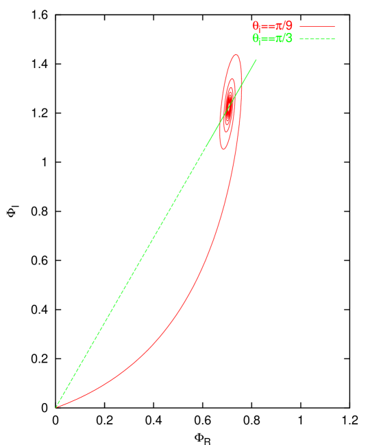
We can see that the initial angle $\theta_{i}$ greatly affects the form of the trajectory for large field values and will lead to different equation of state histories, and hence different amounts of expansion. $N(\theta)$ is shown in Figure 2, where we integrated the equation of motion starting from a fixed small initial value of $\phi$ and continuing until a fixed final energy density where the equations of state had converged .

Figure 2: Number of $e$-folds $N$ as a function of the initial angle $\theta_{\mathrm{i}}$.

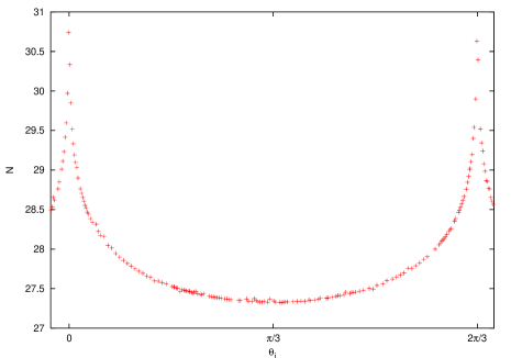
We see that

$$\frac{\partial N}{\partial\theta}\sim{\cal O}(1)$$ (20)

for a wide range of $\theta_{i}$, though the initial values $\theta_{i}\sim 2n\pi/3$, which lead to large spikes in $N$, could be a postiori preferred due to the greater spatial volume produced [12].

Thus, from Eqs. (18) and (19), we see that the angular fluctuations give a comparable, or possibly greater, contribution to the final curvature perturbation. This is due to the huge magnification of the angular fluctuations as $\phi$ rolls from small values to Planckian values, comparable to the usual huge magnification of radial fluctuations near a maximum due to the factor $\partial N/\partial\phi=-H/\dot{\phi}$.

However, as ${\partial N}/\partial\theta$ does not depend on the initial value of $\phi$ (assuming that it is small), ${\partial N}/\partial\theta$ will be independent of $k$. Thus the contribution of the angular fluctuations, Eq. (19), has the same steep spectrum as that of the radial fluctuations and is not consistent with observations.

In the next sections we introduce models which avoid this problem.

4.3 Single Modulus with Quantum Corrections

Here we consider the next simplest model of modular inflation given in Ref. [19]. We first briefly describe the model and then discuss the perturbations produced by it.

The previous model considered a modulus rolling away from a maximum at a point of enhanced symmetry. At such a point of enhanced symmetry, one would in general expect the modulus to have couplings to other light fields. These couplings will cause the mass to renormalise as a function of $\phi$. This could turn the mass squared of the modulus positive for small $\phi$, shifting the maximum of the potential out to some finite value $\phi=\phi_{*}$.

Explicitly, following Ref. [19] with the notation change $\epsilon\rightarrow\beta$ and implicitly keeping the full complex modulus field $\Phi$,

$$V=V_{0}\left[1-\frac{1}{2}\,f(\beta\ln\phi)\,\phi^{2}+\ldots\right]~{},$$ (21)

and we have a maximum at $\phi=\phi_{*}$ where

$$f_{*}+\frac{1}{2}\beta f^{\prime}_{*}=0~{}.$$ (22)

We resolve the ambiguity in the definitions of $f$ and $\beta$ by fixing $f_{*}=f(-1)$ so that $\phi_{*}=e^{-1/\beta}$. Note that $f_{*}<0$ and typically $\beta\ll 1$. We assume $H\simeq\sqrt{V_{0}/3}$ and $\phi\simeq\phi_{*}$ when observable scales leave the horizon.

One will again have eternal inflation at the maximum, which now corresponds to the ring $\phi=\phi_{*}$, and the eternal inflation ends locally when $\phi$ locally rolls off the maximum towards large values. The distribution of $\theta$ values during the eternal inflation could be biased by the small symmetry breaking effects of the $\Phi^{3}$ terms, which should also be included in this model, because the difference in expansion rate around the ring leads to differences in the spatial volumes generated. However, for small $\phi_{*}$, this biasing will be negligible as the differential expansion rate is much smaller than the diffusion rate around the ring due to quantum fluctuations.

This model has the interesting property that in the neighborhood of the maximum the potential is flattened in the radial direction by a factor $\beta$. This helps to flatten the contribution of the radial fluctuations to the final curvature perturbation, but not by as much as one would like [19]. However, we will be more interested in the effect of the shift of the maximum out to finite $\phi=\phi_{*}$. This means that as $\phi$ rolls off the maximum, while $\phi-\phi_{*}\ll\phi_{*}$, the radius $\phi$ will hardly change, allowing the angular fluctuations to give a flat contribution to the final curvature perturbation.

Explicitly, the contribution of the radial fluctuations to final curvature perturbation is

$$\frac{\partial N}{\partial\phi}\,\delta\phi=-\frac{H}{\dot{\phi}}\,\delta\phi\sim\frac{H}{\phi-\phi_{*}}~{},$$ (23)

and the contribution of the angular fluctuations is

$$\frac{\partial N}{\partial\theta}\,\delta\theta\sim\frac{\partial N}{\partial\theta}\frac{H}{\phi}~{}.$$ (24)

Therefore, for $\partial N/\partial\theta\sim\mathcal{O}(1)$, the contribution of the angular fluctuations is suppressed relative to that of the radial fluctuations by the factor $(\phi-\phi_{*})/\phi$. This is easily understood as for large $\phi$, i.e. on small scales, the contributions are comparable, but as one approaches $\phi_{*}$, i.e. going to larger scales, the angular contribution to the spectrum flattens out while the radial contribution continues rising and so dominates.

However, if $\partial N/\partial\theta\gg 1$, then the contribution of the angular fluctuations can dominate the final curvature perturbation giving the desired flat spectrum. This is realized, as indicated from Figure 2, if the angle is close to the one of angular maxima of the potential at $\theta=2n\pi/3$. As mentioned before, this can be probable if we consider that regions corresponding to these initial angles will undergo greater expansion and hence occupy a larger volume at late times. However, we do not want to be drawn too close to these special angles as $\partial N/\partial\theta$ will either diverge or be zero there. This requires further investigation [12].

A more precise formula for the spectrum of $\delta\theta$ is given by Eqs. (52) and (53) in the Appendix. The spectral index has the form

$$n-1=-Ak^{\beta f^{\prime}_{*}}~{},$$ (25)

and the running

$$\frac{dn}{d\ln k}=-A\beta f^{\prime}_{*}k^{\beta f^{\prime}_{*}}~{}.$$ (26)

Therefore, if the contribution of the angular fluctuations dominates, one can expect a flat spectrum on larger scales with the spectrum dipping away with substantial running on smaller scales. It is very plausible that observable scales correspond to $\phi$ close to, but not very close to, $\phi_{*}$, so that this running would be observable [20].

4.4 A Second Modulus

String theory does not predict a single modulus, but rather many moduli. Here, in addition to $\Phi$, we consider the case that there is a second modulus $\Psi$ which drives eternal modular inflation and also some post-eternal modular inflation, before $\Phi$ rolls down driving its own modular inflation.

We take $\Psi$’s potential to have the form

$$V=V_{0}-\frac{1}{2}m_{\psi}^{2}\psi^{2}+\ldots~{},$$ (27)

where we consider just a single real direction $\psi\in\Psi$, and, as always, $m_{\psi}^{2}\sim V_{0}$ and everything is at the vacuum supersymmetry breaking scale. As before, $\psi$ rolls down as

$$\psi\propto a^{\alpha}~{},$$ (28)

where

$$\alpha=\frac{3}{2}\left(\sqrt{1+\frac{4m_{\psi}^{2}}{3V_{0}}}\,-1\right)$$ (29)

and the contribution of fluctuations in $\psi$ to the final curvature perturbation will be

$$\frac{\partial N}{\partial\psi}\,\delta\psi=-\frac{H}{\dot{\psi}}\,\delta\psi\sim\frac{H}{\psi}~{}.$$ (30)

During the modular inflation driven by $\psi$, $\Phi$’s potential will have the form

$$V=V(\psi)+\frac{1}{2}m_{\phi}^{2}(\phi,\psi)\,\phi^{2}+\ldots~{}.$$ (31)

The mass squared $m_{\phi}^{2}(\phi,\psi)$ is renormalised as a function of $\phi$ as before. However, it will also have a dependence on $\psi$ due to the supersymmetry breaking effect of $\psi$’s potential. Schematically, it looks like

$$m_{\phi}^{2}(\phi,\psi)\sim-m_{\mathrm{vac}}^{2}+m_{\mathrm{inf}}^{2}+\beta m_{\mathrm{ren}}^{2}\ln\phi~{},$$ (32)

where $m_{\mathrm{vac}}^{2}\sim m_{\mathrm{inf}}^{2}\sim m_{\mathrm{ren}}^{2}\sim m_{\psi}^{2}$ and $\beta\ll 1$. We assume the indicated signs and that $m_{\mathrm{inf}}^{2}>m_{\mathrm{vac}}^{2}$ so that $m_{\phi}^{2}>0$ at large $\phi$ during $\psi$’s modular inflation. We further assume that the renormalisation group running eventually turns $m_{\phi}^{2}$ negative so that $\phi$ has a minimum at some exponentially small value $\phi_{*}$. This is just the inverse of the running we had in the previous model which produced a maximum, and leads to a quite interesting scenario as follows.

During $\psi$’s modular inflation, $\phi$ has a mass of order $H$ which will suppress its fluctuations , while $\Phi$’s angular component stays massless and so will have unsuppressed fluctuations. Once $\psi$’s modular inflation ends, $m_{\mathrm{inf}}^{2}$ will disappear, or at least change greatly, releasing $\phi$ to roll down to its vacuum at Planckian values as in our previous models, driving some more modular inflation as it does so. The angular fluctuations in $\Phi$ are massively amplified by this roll down and give a contribution to the final curvature perturbation

$$\frac{\partial N}{\partial\theta}\,\delta\theta\sim\frac{\partial N}{\partial\theta}\frac{H}{\phi_{*}}$$ (33)

assuming that observable scales leave the horizon during $\psi$’s modular inflation. Since $\partial N/\partial\theta$ is independent of $k$, and $\phi_{*}$ is a constant, we get a flat contribution to the final curvature perturbation. Furthermore, it will dominate over $\psi$’s contribution as long as $\psi\gg\phi_{*}$ when observable scales leave the horizon. Finally, for $H\sim 10^{-16}$ and $\partial N/\partial\theta\sim\mathcal{O}(1)$, our model matches the COBE normalisation with a very reasonable $\phi_{*}\sim 10^{-12}$, which is a natural consequence of the logarithmic renormalisation group running in our weak coupling regime.

A more precise formula for the spectrum of $\delta\theta$ is given by Eqs. (59) and (60) in the Appendix. The spectral index has the form

$$n-1=-Ak^{2\alpha}~{},$$ (34)

and the running

$$\frac{dn}{d\ln k}=-2\alpha Ak^{2\alpha}~{}.$$ (35)

So, as in our previous model, one can expect a flat spectrum on larger scales with the deviation from a flat spectrum on smaller scales. In this model one expects $\alpha\sim 1$ so the running will typically be larger than in the previous model. Due to the second modular inflation driven by $\phi$, it is very plausible that observable scales left the horizon near the end of the first modular inflation driven by $\psi$, so that this running may be observable [20].

As mentioned in the Appendix, the above formula for the spectral index applies only for $\alpha<1$. The case $\alpha\gtrsim 1$ is more involved because the deviation from scale invariance is dominated by non-trivial dynamics at the end of inflation. Thus, in our model, even though the spectrum will be rather flat on large scales, we could possibly expect deviation from a flat spectrum for smaller scales caused by late-time inflation dynamics affecting super-horizon modes [21]. We leave the detailed analysis of this perturbation calculation on super-horizon scales during the late epoch of modular inflation for our forthcoming paper [12].

5 Thermal Inflation

After our modular inflation, the moduli roll down and oscillate about the minimum of their potential. If this minimum corresponds to a point of enhanced symmetry, where the modulus has unsuppressed couplings to other light fields, then the modulus will decay rapidly. If the minimum is a Planckian distance away from any such point, then the modulus will have only gravitational strength couplings to other light fields and will decay too late for the successful predictions of Big Bang nucleosynthesis to survive [2]. Even if our modulus decays rapidly, one expects other moduli to be displaced during the modular inflation and to roll down and oscillate when it ends. Again, these moduli may either decay rapidly, or contribute to the Polonyi problem. Thus, after the modular inflation, one expects to have initially perhaps comparable fractions of radiation and dangerous long-lived moduli.

Thermal inflation is considered to be one of the most promising mechanisms to get rid of the unwanted moduli. We keep the following discussion of thermal inflation fairly brief and refer the reader to Ref. [11] for more details.

Thermal inflation is driven by a flaton $\sigma$ with potential of the form

$$V=V_{0}+\left(g^{2}T^{2}-m^{2}\right)|\sigma|^{2}+\left(A\lambda\sigma^{n}+\mbox{h.c.}\right)+|\lambda|^{2}|\sigma|^{2n-2}~{},$$ (36)

with $m\sim 10^{2}-10^{3}$ GeV and $n=4$ or $5$. The flaton’s vacuum expectation value is $M\sim m^{1/(n-2)}$ and $V_{0}\sim m^{2}M^{2}\ll m^{2}$ so we do not expect eternal or modular inflation. When $T>T_{\mathrm{c}}=m/g$, the flaton is trapped at the origin by the finite temperature potential, and inflation begins when $V_{0}$ dominates over the moduli density. After about 5 to 10 $e$-folds of inflation, which dilutes the moduli, the temperature drops below $T_{\mathrm{c}}$ and the flaton rolls rapidly towards its minimum ending the inflation. The Universe is then dominated by the oscillating flaton, which eventually decays to ordinary fields through non-renormalisable operators suppressed by of order $M$. After this ‘reheating’ at temperatures of order GeV, standard Big Bang cosmology follows.

We point out here that fluctuations in the angular part of the modulus produced during the modular inflation, which lead to perturbed trajectories at the end of the modular inflation, could lead to perturbations in the fraction of radiation produced at the end of the modular inflation. This could then lead to perturbations in the amount of thermal inflation, as the thermal inflation begins when the moduli density drops below $V_{0}$ but ends when the temperature drops below $T_{\mathrm{c}}$, giving an extra contribution to $\partial N/\partial\theta$. However, the perturbation in the fraction of radiation produced at the end of the modular inflation is likely to be highly model dependent and difficult to evaluate. This will be further investigated in Ref. [12], though we do not expect it to change our conclusions greatly.

We also note in Appendix A.3 that thermal fluctuations can produce perturbations during thermal inflation, but these are negligible in our case.

Thus thermal inflation, which is a natural consequence of thermal effects in the presence of supersymmetric flat directions, resolves our remaining difficulty with modular cosmology.

6 Conclusions

We presented the first realistic modular cosmology scenario in that dilaton stabilization, inflation producing a scale invariant spectrum of density perturbations, and Polonyi/moduli problems are resolved in a simple and self-consistent manner.

One of the notable features is eternal inflation at the vacuum supersymmetry breaking scale. This causes the fine-tuned initial conditions required for the dilaton to find its way to a weak coupling minimum to become a postiori as natural as any others because of the subsequent eternal inflation.

Our model also predicts the observed scale-invariant cosmic microwave background spectrum without any fine-tuning, and even allows for the possibility of a dipping spectrum with significant running on smaller scales [20], which alone could deserve special attention from the viewpoint of inflation model building. Indeed, non-slow-rolling inflaton fields are generic in supergravity theory, but usually avoided by fine-tuning because of their non-scale-invariant power spectrum. This fine-tuning is not necessary in our scenario because the density perturbation is dominantly produced from the angular degree of freedom of a modulus whose usually subdominant fluctuations are hugely amplified by the long roll out of the modulus. We gave explicit calculations of the spectrum, spectral index and its running for modular inflation for concrete toy models. We also pointed out the possible deviation from scale invariance at small scales for some values of the parameters, and we leave thorough treatment of this issue for our forthcoming paper [12].

Finally, thermal inflation solves the Polonyi/moduli problem.

Due to the generic existence of ubiquitous moduli in string/M-theory, an early universe history where moduli play crucial roles would be a rather natural consequence. We kept our discussions fairly general so that it can be applied to a wide class of models, and hope our proposed scenario leaves room for the further investigation of successful modular cosmology.

Acknowledgements

We thank Joanne D. Cohn for catalyzing our collaboration and for encouragement, and the SF02 Cosmology Summer Workshop for hospitality when this collaboration began. E.D.S. thanks the Fermilab Theoretical Astrophysics Group for hospitality while this work was in progress. K.K. thanks J.D. Cohn and H. Murayama for their continuous encouragements. E.D.S. was supported in part by the Astrophysical Research Center for the Structure and Evolution of the Cosmos funded by the Korea Science and Engineering Foundation and the Korean Ministry of Science, and by the Korea Research Foundation grants KRF-2000-015-DP0080 and KRF PBRG 2002-070-C00022. K.K. was supported in part by NSF under grant AST-0205935.

A Appendices

A.1 Precise Calculation of $\delta\theta$

In this appendix we calculate the spectra for the models presented in Sections 4.3 and 4.4, starting with a general formula applicable to both.

To calculate $\delta\theta$, on superhorizon scales but while the angular potential is still flat, we need to solve the perturbed equation of motion for $\delta\theta(k,t)$

$$\frac{d}{dt}\left(a^{3}\phi^{2}\frac{d\,\delta\theta}{dt}\right)+ak^{2}\phi^{2}\delta\theta=0~{}.$$ (37)

Defining

$$\varphi\equiv a\phi\,\delta\theta$$ (38)

and using the conformal time $d\eta\equiv dt/a$, we obtain

$$\frac{d^{2}\varphi}{d\eta^{2}}+\left[k^{2}-\frac{1}{a\phi}\frac{d^{2}(a\phi)}{d\eta^{2}}\right]\varphi=0~{},$$ (39)

where

$$\frac{1}{a\phi}\frac{d^{2}(a\phi)}{d\eta^{2}}=2a^{2}H^{2}\left(1+\frac{1}{2H^{2}}\frac{dH}{dt}+\frac{3}{2H\phi}\frac{d\phi}{dt}+\frac{1}{2H^{2}\phi}\frac{d^{2}\phi}{dt^{2}}\right)~{}.$$ (40)

Introducing $y\equiv\sqrt{2k}\,\varphi$ and $x\equiv-k\eta$, we can write this as

$$\frac{d^{2}y}{dx^{2}}+\left(1-\frac{2}{x^{2}}\right)y=\frac{g}{x^{2}}y~{},$$ (41)

where

$$g=\frac{1}{xa\phi}\left[\frac{d^{2}(xa\phi)}{(d\ln x)^{2}}-3\frac{d(xa\phi)}{d\ln x}\right]~{}.$$ (42)

For

$$g=\xi\left(\frac{x}{x_{\star}}\right)^{\nu}$$ (43)

with $\xi\ll 1$, this can be solved to give [22]

$$P_{\delta\theta}(k)=\left(\frac{k}{2\pi x_{\star}a_{\star}\phi_{\star}}\right)^{2}\left\{1+\frac{2}{(3-\nu)\nu}\left[(2x_{\star})^{-\nu}\cos\left(\frac{\pi\nu}{2}\right)\frac{\Gamma(2+\nu)}{1-\nu}-1\right]\xi+{\cal O}(\xi^{2})\right\}~{},$$ (44)

where subscript $\star$ denotes an appropriate evaluation point. The divergence at $\nu=-2$ corresponds to the deviation of the spectrum from scale invariance being dominated by late time dynamics [21]. The spectral index is

$$n_{\delta\theta}(k)-1=-\cos\left(\frac{\pi\nu}{2}\right)\frac{2\Gamma(2+\nu)}{(1-\nu)(3-\nu)}\frac{\xi}{(2x_{\star})^{\nu}}~{}.$$ (45)

We apply the above formula to the specific models we discussed in the paper.

A.1.1 Single Modulus with Quantum Corrections

Here we derive the explicit form for Eq. (25) of Section 4.3.

For $H\simeq\sqrt{V_{0}/3}\,$, we have

$$x=\frac{k}{aH}~{},$$ (46)

and

$$g=\frac{3}{\phi H}\frac{d\phi}{dt}+\frac{1}{\phi H^{2}}\frac{d^{2}\phi}{dt^{2}}~{}.$$ (47)

Eq. (24) of Ref. [19] gives

$$\ln\left(\frac{\phi}{\phi_{*}}\right)=\frac{1}{\beta}e^{-\beta f^{\prime}_{*}(N+C)}~{},$$ (48)

where $N$ is the number of $e$-folds until inflation ends at $\phi\sim 1$, and $C\sim 1/\beta$. Therefore

$$\frac{1}{\phi H}\frac{d\phi}{dt}=f^{\prime}_{*}e^{-\beta f^{\prime}_{*}(N+C)}$$ (49)

and

$$\frac{1}{\phi H^{2}}\frac{d^{2}\phi}{dt^{2}}=f^{\prime}_{*}e^{-\beta f^{\prime}_{*}(N+C)}\left[\beta f^{\prime}_{*}+f^{\prime}_{*}e^{-\beta f^{\prime}_{*}(N+C)}\right]\simeq\beta{f^{\prime}_{*}}^{2}e^{-\beta f^{\prime}_{*}(N+C)}~{}.$$ (50)

Hence

$$g=\left(3+\beta f^{\prime}_{*}\right)f^{\prime}_{*}e^{-\beta f^{\prime}_{*}(N+C)}=\left(3+\beta f^{\prime}_{*}\right)\beta f^{\prime}_{*}\ln\left(\frac{\phi_{\star}}{\phi_{*}}\right)\left(\frac{x}{x_{\star}}\right)^{-\beta f^{\prime}_{*}}~{},$$ (51)

leading to

$$P_{\delta\theta}(k)=\left(\frac{H_{\star}}{2\pi\phi_{\star}}\right)^{2}\left\{1-2\left[2^{\beta f^{\prime}_{*}}\cos\left(\frac{\pi\beta f^{\prime}_{*}}{2}\right)\frac{\Gamma(2-\beta f^{\prime}_{*})}{1+\beta f^{\prime}_{*}}\left(\frac{k}{a_{\star}H_{\star}}\right)^{\beta f^{\prime}_{*}}-1\right]\ln\left(\frac{\phi_{\star}}{\phi_{*}}\right)\right\}$$ (52)

and

$$n_{\delta\theta}(k)-1=-2^{\beta f^{\prime}_{*}}\cos\left(\frac{\pi\beta f^{\prime}_{*}}{2}\right)\frac{\Gamma(2-\beta f^{\prime}_{*})}{(1+\beta f^{\prime}_{*})}2\beta f^{\prime}_{*}\ln\left(\frac{\phi_{\star}}{\phi_{*}}\right)\left(\frac{k}{a_{\star}H_{\star}}\right)^{\beta f^{\prime}_{*}}~{}.$$ (53)

Note the sign change from one’s naive expectation for $\beta f^{\prime}_{*}>1$ [12].

A.1.2 A Second Modulus

Now we derive the explicit form for Eq. (34) of Section 4.4.

Here we assume $\phi=\phi_{*}$ leaving consideration of the effects of any time dependence of $\phi$ to another paper [12]. $\psi$ scales as

$$\psi\propto a^{\alpha}$$ (54)

with

$$\alpha=\frac{3}{2}\left(\sqrt{1+\frac{4m_{\psi}^{2}}{3V_{0}}}\,-1\right)~{}.$$ (55)

Therefore

$$3H^{2}=V_{0}-\frac{1}{2}m_{\psi}^{2}\psi^{2}+\frac{1}{2}\dot{\psi}^{2}=V_{0}\left(1-\frac{1}{2}\alpha\psi^{2}\right)$$ (56)

and

$$x=\frac{k}{aH}\left[1+\frac{\alpha^{2}\psi^{2}}{2(1-2\alpha)}\right]~{}.$$ (57)

Hence

$$g=\frac{1}{2}\left(\frac{3+2\alpha}{1-2\alpha}\right)\alpha^{2}\psi_{\star}^{2}\left(\frac{x}{x_{\star}}\right)^{-2\alpha}~{},$$ (58)

leading to

$$P_{\delta\theta}(k)=\left(\frac{H_{\star}}{2\pi\phi_{*}}\right)^{2}\left\{1-\frac{\alpha}{2}\left[2^{2\alpha}\cos(\pi\alpha)\frac{\Gamma(2-2\alpha)}{1-4\alpha^{2}}\left(\frac{k}{a_{\star}H_{\star}}\right)^{2\alpha}-1\right]\psi_{\star}^{2}\right\}$$ (59)

and

$$n_{\delta\theta}(k)-1=-2^{2\alpha}\cos(\pi\alpha)\frac{\Gamma(2-2\alpha)}{1-4\alpha^{2}}\alpha^{2}\psi_{\star}^{2}\left(\frac{k}{a_{\star}H_{\star}}\right)^{2\alpha}~{}.$$ (60)

A.2 Estimation of the Required Value of $\partial N/\partial\theta$ for the Single Modulus with Quantum Corrections Model

In the single modulus with quantum corrections model of Section 4.3, the radial fluctuations have only a slightly flattened spectrum. Therefore we require

$$\frac{\partial N}{\partial\phi}\,\delta\phi\lesssim 10^{-1}\frac{\partial N}{\partial\theta}\,\delta\theta$$ (61)

to avoid the radial fluctuations giving the full spectrum too big a deviation from scale invariance. Now

$$\delta\theta\sim\frac{\dot{\phi}}{H\phi}\frac{\partial N}{\partial\phi}\,\delta\phi$$ (62)

and using the results of Appendix A.1.1 we have

$$\frac{\dot{\phi}}{H\phi}\sim\beta f^{\prime}_{*}\ln\left(\frac{\phi}{\phi_{*}}\right)\sim\frac{n_{\delta\theta}-1}{2}\lesssim 10^{-2}~{}.$$ (63)

Thus we get the estimate

$$\frac{\partial N}{\partial\theta}\gtrsim 10^{3}~{}.$$ (64)

We also note that matching the COBE normalization requires

$$\frac{\partial N}{\partial\theta}\frac{H}{\phi_{*}}\sim 10^{-4}~{},$$ (65)

and so for $H\sim 10^{-16}$ require

$$\frac{\partial N}{\partial\theta}\sim 10^{12}\phi_{*}$$ (66)

which gives us an upper limit on $\partial N/\partial\theta$ as we expect $\phi_{*}$ to be well below the Planck scale.

A.3 Perturbations from Thermal Fluctuations during Thermal Inflation

In this appendix we note that there can arise another source of perturbations caused by thermal fluctuations during thermal inflation. These thermal fluctuations can be estimated by considering the thermal fluctuation $\delta T\sim T$ in regions of the thermal bath of size $\sim 1/T$. A Hubble volume of radius $1/H$, outside of which the thermal fluctuation freezes in, encloses $T^{3}/H^{3}$ of such regions giving a thermal fluctuation on the Hubble scale of $\delta T\sim T/\sqrt{T^{3}/H^{3}}$. Thus we have

$$\mathcal{R}_{\mathrm{c}}=\delta N=\frac{\partial N}{\partial T}\,\delta T\sim\frac{1}{T}\cdot T\sqrt{\frac{H^{3}}{T^{3}}}\sim\left(\frac{T_{\mathrm{c}}M}{T}\right)^{3/2}~{}.$$ (67)

Now $T\propto a^{-1}$ and so this has a spectral index $n=4$, with its maximum value $\sim M^{3/2}$ at the end of thermal inflation. This is completely negligible for thermal inflation with an intermediate scale $M$ as we are considering, but could be significant for thermal inflation driven by a flaton with $M\gtrsim M_{\mathrm{GUT}}$.

References

- [1] See for example: P. Binetruy and M.K. Gaillard, Phys. Rev. D34, 3069 (1986); F.C. Adams, J.R. Bond, K. Freese, J.A. Frieman and A.V. Olinto, Phys. Rev. D47 (1993) 426; L. Randall and S. Thomas, Nucl. Phys. B449, 229 (1995), hep-ph/9407248; T. Banks, M. Berkooz, S.H. Shenker, G.W. Moore and P.J. Steinhardt, Phys. Rev. D52, 3548 (1995), hep-th/9503114; L. Randall, M. Soljacic and A.H. Guth, Nucl. Phys. B472 (1996) 377.
- [2] G.D. Coughlan, W. Fischler, E.W. Kolb, S. Raby and G.G. Ross, Phys. Lett. B131, 59 (1983); T. Banks, D.B. Kaplan and A.E. Nelson, Phys. Rev. D49, 779 (1994), hep-ph/9308292; B. de Carlos, J.A. Casas, F. Quevedo and E. Roulet, Phys. Lett. B318, 447 (1993), hep-ph/9308325.
- [3] M. Dine and N. Seiberg, Phys. Lett. B162, 299 (1985).
- [4] R. Brustein and P.J. Steinhardt, Phys. Lett. B302, 196 (1993), hep-th/9212049.
- [5] A.D. Linde, Inflation and Quantum Cosmology, ed. R. Brandenberger (Academic Press, 1990).
- [6] M. Sasaki and E.D. Stewart, Prog. Theor. Phys. 95, 71 (1996), astro-ph/9507001.
- [7] N.V. Krasnikov, Phys. Lett.B193, 37 (1987). L.J. Dixon, Talk given at 15th APS Div. of Particles and Fields General Mtg., Houston, TX, Jan 3-6, 1990. Published in DPF Conf. 811 (1990), SLAC-PUB-5229, 1990.
- [8] A.H. Guth, Phy. Rev. D 23, 347 (1981); J.R. Gott, Nature 295, 304 (1982); K. Sato, H. Kodama, M. Sasaki, and M. Maeda, Phy. Lett. B 108, 103 (1982).
- [9] A.D. Linde, Phys. Lett. B108, 389 (1982); A. Albrecht and P.J. Steinhardt, Phys. Rev. Lett. 48, 1220 (1982); P.J. Steinhardt in: The Very Early Universe, eds. G.Gibbons, S.W. Hawking and S.T.C. Siklos; A. Vilenkin, Phys. Rev. D 27, 2848 (1983).
- [10] E.D. Stewart, talk given at Cosmo 2000, Cheju Island, Korea, 4-8 Sep. 2000, published in Cosmo 2000 Proceedings, eds. P. Ko, K. Lee and J.E. Kim (World Scientific, 2001) 147, also available at http://astro-kaist.info/.
- [11] D.H. Lyth and E.D. Stewart, Phys. Rev. Lett.75 (1995) 201, hep-ph/9502417; Phys. Rev. D53 (1996) 1784, hep-ph/9510204.
- [12] K. Kadota and E.D. Stewart, to appear.
- [13] E.D. Stewart, ‘Introduction to Inflationary Cosmology’, Lectures presented at the 8th Mini-Workshop on Particle and Astroparticle Physics, Pusan National University, Pusan, Korea, 22-24 May 1997.
- [14] E.D. Stewart and D.H. Lyth, Phys. Lett. B302, 171 (1993), gr-qc/9302019.
- [15] A.R. Liddle and D.H. Lyth, Phys. Rep. 231 1 (1993), astro-ph/9303019.
- [16] E.J. Copeland, A.R. Liddle, D.H. Lyth, E.D. Stewart and D. Wands, Phys. Rev. D49, 6410 (1994), astro-ph/9401011.
- [17] E.D. Stewart, Phys. Rev. D51 (1995) 6847, hep-ph/9405389.
- [18] D.H. Lyth and D. Wands, Phys. Lett. B524, 5 (2002), hep-ph/0110002; T. Moroi and T. Takahashi, Phys. Lett. B522, 215 (2001): Erratum-ibid. B539, 303 (2002), hep-ph/0110096.
- [19] E.D. Stewart, Phys. Lett. B391, 34 (1997), hep-ph/9606241.
- [20] C.L. Bennett et al., astro-ph/0302207.
- [21] S.M. Leach, M. Sasaki, D. Wands and A.R Liddle, Phys. Rev. D64, 023512 (2001), astro-ph/0101406.
- [22] E.D. Stewart, Phys. Rev. D65, 103508 (2002), astro-ph/0110322.