TU-684

hep-ph/0304126

April, 2003

Cosmic String from $D$-term Inflation and Curvaton

Motoi Endo^(a), Masahiro Kawasaki^(b) and Takeo Moroi^(a)

^(a)Department of Physics, Tohoku University
Sendai 980-8578, Japan

^(b)Research Center for the Early Universe, School of Science, University of Tokyo
Tokyo 113-0033, Japan

We study effects of the cosmic string in the $D$-term inflation model on the cosmic microwave background (CMB) anisotropy. In the $D$-term inflation model, gauged cosmic string is usually formed, which may significantly affect the CMB anisotropy. We see that its study imposes important constraint. In order to realize the minimal model of $D$-term inflation, we see that the coupling constant $\lambda$ in the superpotential generating the inflaton potential should be significantly small, $\lambda\mathop{}_{\textstyle\sim}^{\textstyle<}O(10^{-4}-10^{-5})$. We also discuss that a consistent scenario of the $D$-term inflation with $\lambda\sim 1$ can be constructed by adopting the curvaton mechanism where the cosmic density fluctuations are generated by a primordial fluctuation of a late-decaying scalar field other than the inflaton.

Inflation [1, 2] provides elegant solutions to many of serious problems in cosmology. As is well known, assuming the de Sitter expansion of the universe in an early epoch, horizon and flatness problems are solved since, during the inflation, physical scale grows much faster than the horizon scale. In addition, quantum fluctuation during the inflation is now a very promising candidate of the origin of the cosmic density fluctuations.

From a particle-physics point of view, thus, it is important to find natural and consistent models of inflation; indeed, many models of inflation have been proposed so far. It is, however, non-trivial to construct a realistic model of inflation. This is because the potential of the inflaton, which is the scalar field responsible for the inflation, is usually required to be very flat although, in general, it is non-trivial to find a natural mechanism to guarantee the flatness of the scalar potential.

Primarily, flatness of the scalar potential is disturbed by loop effects. In particular, quadratic divergences usually show up once one calculates radiative corrections to the scalar mass and hence scalar fields lighter than the cut-off scale (which is naturally of the order of the gravitational scale) is hard to realize in a general framework. This difficulty can be relatively easily avoided by introducing supersymmtry which we assume in this paper. Even in the supersymmetric framework, however, it is still difficult to find a realistic model of inflation since, in the de Sitter background, supergravity effects may induce effective mass as large as the expansion rate during the inflation (i.e., so called “Hubble-induced mass”) to scalar fields, which spoils the flatness of the inflaton potential.

One elegant solution to the problem of the Hubble-induced mass is to adopt the $D$-term inflation [3, 4]. Since the Hubble-induced mass originates from $F$-term interactions, inflaton potential is free from this problem if the vacuum energy during the inflation is provided only by a $D$-term interaction, which is the case in the $D$-term inflation model.

In the $D$-term inflation, a U(1) gauge interaction is introduced to realize a flat potential of the inflaton. Inflation proceeds in the symmetric phase of the U(1) while, after the inflation, the U(1) symmetry is broken by a vacuum expectation value of one of scalar fields in the model. Since the U(1) gauge symmetry is spontaneously broken, gauged string arises in this framework and hence the $D$-term inflation inevitably predicts the existence of the cosmic string [5, 6]. If the cosmic string is formed, it affects the CMB anisotropy and changes the shape of the CMB angular power spectrum $C_{l}$ [7, 8], which is defined as

$$\left\langle\Delta T(\vec{x},\vec{\gamma})\Delta T(\vec{x},\vec{\gamma}^{\prime})\right\rangle_{\vec{x}}=\frac{1}{4\pi}\sum_{l}(2l+1)C_{l}P_{l}(\vec{\gamma}\cdot\vec{\gamma}^{\prime}),$$ (1)

with $\Delta T(\vec{x},\vec{\gamma})$ being the temperature fluctuation of the CMB radiation pointing to the direction $\vec{\gamma}$ at the position $\vec{x}$ and $P_{l}$ being the Legendre polynomial. If the effect of the cosmic string on the CMB anisotropy is too strong, the CMB angular power spectrum may become inconsistent with the observations since the observed values of $C_{l}$ is highly consistent with that from purely adiabatic density fluctuations which is the prediction of the “usual” inflation models without cosmic string.

In this paper, we study effects of the cosmic string in the framework of the $D$-term inflation paying particular attention to its effects on the CMB anisotropy. Taking account of the effect of the cosmic string, we see that the CMB angular power spectrum may become significantly deviate from the usual adiabatic results. Using the recent precise measurement of the CMB angular power spectrum by the WMAP [9], we derive constraints on the $D$-term inflation scenario. As a result, we see that the coupling constant $\lambda$ in the superpotential generating the inflaton potential should be $O(10^{-4}-10^{-5})$ or smaller. We also discuss that a consistent scenario of the $D$-term inflation with $\lambda\sim 1$ is possible by adopting the curvaton mechanism [10, 11, 12, 13] where primordial amplitude fluctuation of a late-decaying scalar condensation (so-called curvaton) becomes the dominant origin of the cosmic density fluctuations.

Let us start our discussion with a brief review of the $D$-term inflation. In the $D$-term inflation models, a new U(1) gauge interaction is introduced, with three chiral superfields, $S(0)$, $\bar{Q}(-1)$ and $Q(+1)$ where we denote the U(1) charges of the superfields in the parenthesis. With the superpotential

$$W=\lambda S\bar{Q}Q,$$ (2)

and adopting non-vanishing Fayet-Illiopoulos $D$-term parameter $\xi$, the scalar potential is given by

$$V=\lambda^{2}\left(|S\bar{Q}|^{2}+|SQ|^{2}+|\bar{Q}Q|^{2}\right)+\frac{1}{2}g^{2}\left(-|\bar{Q}|^{2}+|Q|^{2}-\xi\right)^{2},$$ (3)

where $g$ is the gauge coupling constant. In our study, we take $\xi$ to be positive (although the final result is independent of this assumption). Minimizing the potential, the true vacuum is given by

$$\langle S\rangle=0,~{}~{}~{}\langle\bar{Q}\rangle=0,~{}~{}~{}\langle Q\rangle=\sqrt{\xi}.$$ (4)

Although the true vacuum is given by (4), there is a (quasi) flat direction, that is, $S\rightarrow\infty$ with $\bar{Q}$ and $Q$ being vanished. Indeed, in this limit, the scalar potential becomes $V=\frac{1}{2}g^{2}\xi^{2}$ and hence, at the tree level, the scalar potential becomes constant. This flat direction is used as the inflaton.

Once the radiative corrections are taken into account, the flat direction is slightly lifted. When the scalar field $S$ takes large amplitude, $\bar{Q}$ and $Q$ become massive and decouple from the effective theory at the energy scale $\lambda S$. This fact means that the gauge coupling constant in this case should be evaluated at the scale $\lambda S$ and hence, for $S\gg g\sqrt{\xi}/\lambda$, $V(S)=\frac{1}{2}g^{2}(\lambda S)\xi^{2}$. Using one-loop renormalization group equation, and defining

$$S=\frac{1}{\sqrt{2}}\sigma e^{i\theta},$$ (5)

the potential for the real scalar field $\sigma$ is given by

$$V(\sigma)=\frac{g^{2}}{2}\xi^{2}+\frac{g^{4}\xi^{2}}{8\pi^{2}}\log\frac{\sigma}{\sigma_{0}},$$ (6)

where $\sigma_{0}$ is some constant.

Since the scalar field $\sigma$ has a very flat potential when $\sigma$ is large, the $\sigma$ field can be used as an inflaton; inflation occurs if $\sigma$ has large enough amplitude. Assuming the slow-roll condition, evolution of the $\sigma$ field during the inflation is described as

$$\sigma^{2}=\sigma_{\rm end}^{2}+\frac{g^{2}}{2\pi^{2}}N_{e}M_{*}^{2},$$ (7)

where $N_{e}$ is the $e$-folds of the inflation and $M_{*}\simeq 2.4\times 10^{18}\ {\rm GeV}$ is the reduced Planck scale. The cosmic density fluctuations responsible for the CMB anisotropy measured by the WMAP (and other) experiment are generated when $N_{e}\sim 30-50$. (Hereafter, we take $N_{e}=50$ in evaluating $C_{l}$.) In addition, $\sigma_{\rm end}$ is the inflaton amplitude at the end of the inflation. In order to realize the $D$-term inflation, $\sigma$ should be large enough so that (i) the slow-roll condition is satisfied and (ii) the effective mass squared of the $Q$ field becomes positive. Inflation ends one of these conditions are violated and hence $\sigma_{\rm end}$ is estimated as

$$\sigma_{\rm end}={\rm max}(\sigma_{\rm s.r.},\sigma_{\rm inst}),$$ (8)

where

$$\sigma_{\rm s.r.}\simeq\frac{g}{2\pi}M_{*},~{}~{}~{}\sigma_{\rm inst}\simeq\frac{\sqrt{2}g}{\lambda}\sqrt{\xi}.$$ (9)

Notice that $\sigma_{\rm s.r.}$ and $\sigma_{\rm inst}$ are derived from the slow-roll condition and the instability of the potential of $Q$, respectively.

Once the evolution of the inflaton field is understood, we can calculate the metric perturbation $\Psi$ generated from the primordial fluctuation of the inflaton field. The metric perturbation after the inflation is proportional to the following quantity [21]:

$${\cal R}^{\rm(inf)}\equiv\frac{H_{\rm inf}}{2\pi}\frac{3H_{\rm inf}^{2}}{(\partial V/\partial\sigma)}=\sqrt{\frac{2}{3}}\pi\frac{\xi}{gM_{*}^{3}}\sigma,$$ (10)

where $H_{\rm inf}$ is the expansion rate during the inflation. (Here and hereafter, the superscript “(inf)” implies that the quantity is induced from the fluctuation of the inflaton field.) Importantly, ${\cal R}^{\rm(inf)}$ changes its behavior at $\lambda\sim\lambda_{\rm crit}$ with

$$\lambda_{\rm crit}\equiv\frac{2\pi}{\sqrt{N_{e}}}\frac{\sqrt{\xi}}{M_{*}}.$$ (11)

When $\lambda\gg\lambda_{\rm crit}$, the second term in the right-hand side of Eq. (7) dominates over the first term and hence $\sigma$ for corresponding $N_{e}$ is given by $gM_{*}\sqrt{N_{e}}/\sqrt{2}\pi$. On the contrary, if $\lambda\ll\lambda_{\rm crit}$, the first term wins and $\sigma\simeq\sigma_{\rm inst}$. As a result, we obtain

$${\cal R}^{\rm(inf)}\simeq\frac{1}{\sqrt{3}}\frac{\xi}{M_{*}^{2}}\sqrt{N_{e}}\times\left\{\begin{array}[]{ll}1&~{}~{}~{}:~{}~{}~{}\lambda\gg\lambda_{\rm crit}\\ (\lambda/\lambda_{\rm crit})^{-1}&~{}~{}~{}:~{}~{}~{}\lambda\ll\lambda_{\rm crit}\end{array}\right..$$ (14)

When $\lambda\gg\lambda_{\rm crit}$, ${\cal R}^{\rm(inf)}$ is proportional to $\xi$ and is independent of $\lambda$. On the contrary, if $\lambda\ll\lambda_{\rm crit}$, ${\cal R}^{\rm(inf)}$ is proportional to $\xi^{3/2}/\lambda$. This fact implies that, for a fixed value of $\xi$, the metric perturbation generated from the inflaton fluctuation is enhanced for sufficiently small value of $\lambda$.

Once the non-vanishing metric perturbation is generated, it becomes an origin of the cosmic density fluctuations. One important point is that the density fluctuations associated with ${\cal R}^{\rm(inf)}$ are purely adiabatic. Notice that the metric perturbation depends on time and, for superhorizon modes, the metric perturbation in the radiation dominated epoch is given by

$$\Psi^{\rm(inf)}_{\rm RD}=\frac{2}{3}{\cal R}^{\rm(inf)}.$$ (15)

(Here and hereafter, the subscript “RD” is for quantities in the radiation dominated epoch.)

After the inflation, scalars settle to the values given in (4). Thus, the gauged U(1) symmetry is spontaneously broken and the cosmic string is formed. The mass per unit length of the string is given by

$$\mu=2\pi\xi.$$ (16)

Once the cosmic-string network is formed, it affects the cosmic density fluctuations. In particular, an important constraint is obtained by studying its effects on the CMB anisotropy. The perturbations induced by cosmic strings are non-Gaussian and decoherent isocurvature, which leads to characteristic spectrum of the CMB anisotropy, which is distinguished from that induced by inflation.

The CMB angular power spectrum in the $D$-term inflation scenario contains two contributions: one is the adiabatic one from the primordial fluctuation of the inflaton and the other is from the cosmic string. Assuming no correlation between these two contributions, we obtain

$$C_{l}=C_{l}^{\rm(inf)}+C_{l}^{\rm(str)},$$ (17)

where $C_{l}^{\rm(inf)}$ and $C_{l}^{\rm(str)}$ are contributions from primordial inflaton fluctuation and cosmic string, respectively. The adiabatic part $C_{l}^{\rm(inf)}$ can be calculated with the conventional method; we use the CMBFAST package [23] to calculate $C_{l}^{\rm(inf)}$. (In our study, we use the cosmological parameters $\Omega_{b}h^{2}=0.024$, $\Omega_{m}h^{2}=0.14$, $h=0.72$, and $\tau=0.166$, where $\Omega_{b}$ and $\Omega_{m}$ are density parameters of baryon and non-relativistic matter, respectively, $h$ the Hubble constant in units of 100 km/sec/Mpc, and $\tau$ the optical depth, which are suggested from the WMAP experiment [24]. It should be noted that these may not necessarily be the best-fit values in the $D$-term inflation case. Varying of these parameters within the reasonable ranges, however, does not change our main conclusion.) Since $C_{l}^{\rm(inf)}$ is from the two point correlation function, the CMB angular power spectrum is second order in density $\Psi^{\rm(inf)}$. In particular, $C_{l}^{\rm(inf)}$ is proportional to $\xi^{2}$ and $\xi^{3}/\lambda^{2}$ for $\lambda\gg\lambda_{\rm crit}$ and $\lambda\ll\lambda_{\rm crit}$, respectively. In addition, the cosmic string contribution $C_{l}^{\rm(str)}$ is proportional to $\mu^{2}\propto\xi^{2}$ [25].

For quantitative studies on the effects of the cosmic string, $l$-dependence of $C_{l}^{\rm(str)}$ should be known. Usually numerical methods are used for this purpose but, unfortunately, it is rather difficult to determine the detailed shape of $C_{l}^{\rm(str)}$; there are two classes of results which give different $l$-dependence of $C_{l}^{\rm(str)}$. One class of results show relatively “flat” behavior of the CMB angular power spectrum [26, 27, 28]; that is, $l(l+1)C_{l}^{\rm(str)}$ is found to be almost constant (at least up to the multipole $l\sim 300$ [27]). However, another class of studies result in “tilted” behavior [29, 30, 31, 32]; the function $\sqrt{l(l+1)C_{l}^{\rm(str)}}$ approximately has a linear dependence on $\log l$ up to $l\sim 400-600$ then it steeply decreases. There is still some discussion on this issue and it has not been clearly understood how $C_{l}^{\rm(str)}$ behaves.

Thus, in our study, we consider both cases adopting some approximate formulae of $C_{l}^{\rm(str)}$. For the flat case, shape of $C_{l}^{\rm(str)}$ at high multipole is quite uncertain. Thus, assuming a dumping behavior at multipole higher than $l_{\rm max}$, we parameterize the cosmic-string contribution as

$$l(l+1)C_{l}^{\rm(str)} = \left\{\begin{array}[]{ll}A^{\rm(str)}_{\rm SW}T_{\rm CMB}^{2}(G\mu)^{2}&~{}~{}~{}:~{}~{}~{}l\leq l_{\rm max}\\ 0&~{}~{}~{}:~{}~{}~{}l>l_{\rm max}\end{array}\right..$$ (20)

Numerical calculation suggests $l_{\rm max}\mathop{}_{\textstyle\sim}^{\textstyle>}300$ [27]. On the contrary, for the tilted case, we use the formula

$$l(l+1)C_{l}^{\rm(str)} = A^{\rm(str)}_{\rm SW}T_{\rm CMB}^{2}(G\mu)^{2}$$ (23)

$$\times\left\{\begin{array}[]{ll}\left[1+a_{l<l_{\rm kink}}\log(l/10)\right]^{2}&~{}~{}~{}:~{}~{}~{}l\leq l_{\rm kink}\\ \left[1+a_{l<l_{\rm kink}}\log(l_{\rm kink}/10)+a_{l>l_{\rm kink}}\log(l/l_{\rm kink})\right]^{2}&~{}~{}~{}:~{}~{}~{}l>l_{\rm kink}\end{array}\right.,$$

where $l_{\rm kink}$ is the multipole above which $C_{l}^{\rm(str)}$ is suppressed for the tilted case. Numerical results suggest $l_{\rm kink}\sim 400-600$, and we use $l_{\rm kink}=500$ in our following discussion. In addition, hereafter, we take $a_{l>500}=-0.6$. The values of $A^{\rm(str)}_{\rm SW}$ and $a_{l<l_{\rm kink}}$ (for the tilted case) found in the literatures are listed in Table 1. As one can see, although the numerical values for $A^{\rm(str)}_{\rm SW}$ are fairly scattered, $A^{\rm(str)}_{\rm SW}$ is found to be $\sim O(100)$.

$A_{\rm str}$	$a_{l<l_{\rm kink}}$	Ref.
$130-350$	$\sim 0$ (flat)	[26, 27]
$\sim 700$	$\sim 0$ (flat)	[28]
$\sim 700$	$0.24-0.34$	[29]
$\sim 600$	$0.26-0.49$	[31]
$\sim 500$	$0.18-0.23$	[32]

Table 1: Values of $A^{\rm(str)}_{\rm SW}$ and $a_{l<l_{\rm kink}}$ found in the literatures. (See Eqs. (20) and (LABEL:Cl^str(tilted)).)

With Eqs. (20) and (LABEL:Cl^str(tilted)), effect of the cosmic string on the Sachs-Wolfe (SW) tail is given by

$$[l(l+1)C_{l}^{\rm(str)}]_{l=10}\simeq 2.2\times 10^{3}{\rm\mu K}^{2}\times\left(\frac{\sqrt{\xi}}{10^{16}{\rm GeV}}\right)^{4}\left(\frac{A^{\rm(str)}_{\rm SW}}{100}\right),$$ (25)

while the inflaton contribution is found to be

$$[l(l+1)C_{l}^{\rm(inf)}]_{l=10}\simeq 2.1\times 10^{3}{\rm\mu K}^{2}\times\left(\frac{\sqrt{\xi}}{10^{16}{\rm GeV}}\right)^{4}\times{\rm max}[1,(\lambda/\lambda_{\rm crit})^{-2}].$$ (26)

Thus, the CMB angular power spectrum is expected to be significantly affected by the cosmic string contribution (at least at the SW tail) assuming $A^{\rm(str)}_{\rm SW}\mathop{}_{\textstyle\sim}^{\textstyle>}O(100)$, unless $\lambda\ll\lambda_{\rm crit}$. This fact implies that the parameter $\lambda$ plays a significant role in determining the shape of the total angular power spectrum. For a given value of $\xi$, $\Psi^{\rm(inf)}$ is more enhanced as $\lambda$ decreases. Thus, when $\lambda\ll\lambda_{\rm crit}$, $C_{l}$ can be dominated by the inflaton contribution and hence it (almost) agrees with the adiabatic result. If $\lambda$ is larger than $\lambda_{\rm crit}$, on the contrary, $C_{l}^{\rm(inf)}$ and $C_{l}^{\rm(str)}$ are both proportional to $\xi^{2}$ and are independent of $\lambda$. Thus, relative size of the inflaton and cosmic-string contributions are fixed in this case.

The CMB angular power spectrum measured by the WMAP is well explained by the adiabatic result [9]. Thus, based on the fact that $C_{l}^{\rm(inf)}$ and $C_{l}^{\rm(str)}$ have different $l$-dependence, the cosmic-string contribution should not be too large. Defining

$$\tilde{A}^{\rm(str)}_{\rm SW}\equiv\left[\frac{\Psi^{\rm(inf)}}{\Psi^{\rm(inf)}|_{\lambda\gg\lambda_{\rm crit}}}\right]^{-2}A^{\rm(str)}_{\rm SW},$$ (27)

the total angular power spectrum is determined by this quantity up to the normalization since $C_{l}^{\rm(str)}\propto A^{\rm(str)}_{\rm SW}\mu^{2}\propto A^{\rm(str)}_{\rm SW}[\Psi^{\rm(inf)}|_{\lambda\gg\lambda_{\rm crit}}]^{2}$ while $C_{l}^{\rm(inf)}\propto[\Psi^{\rm(inf)}]^{2}$. Notice that $\tilde{A}^{\rm(str)}_{\rm SW}\simeq A^{\rm(str)}_{\rm SW}$ for $\lambda\mathop{}_{\textstyle\sim}^{\textstyle>}\lambda_{\rm crit}$ while $\tilde{A}^{\rm(str)}_{\rm SW}\simeq(\lambda/\lambda_{\rm crit})^{2}A^{\rm(str)}_{\rm SW}$ for $\lambda\mathop{}_{\textstyle\sim}^{\textstyle<}\lambda_{\rm crit}$.

Figure 1: The $\chi^{2}$ variable as a function of $A_{\rm str}$ for the flat case with $l_{\rm max}=300$ (solid) and tilted case with $a_{l<500}=0.2$ (dotted) and $0.4$ (dashed).

With the approximated formulae (20) and (LABEL:Cl^str(tilted)), we calculate the $\chi^{2}$ variable as a function of $\tilde{A}^{\rm(str)}_{\rm SW}$ and $\xi$ (or equivalently, ${\cal R}^{\rm(inf)}$) using the likelihood code provided by the WMAP collaboration [33] with the WMAP data [9]. For a fixed value of $\tilde{A}^{\rm(str)}_{\rm SW}$, we vary $\xi$ and obtain the minimal value of $\chi^{2}$, which we call $\chi^{2}_{\rm min}(\tilde{A}^{\rm(str)}_{\rm SW})$. We checked that the $\chi^{2}$ variable has its minimum value when $\tilde{A}^{\rm(str)}_{\rm SW}$ is small enough, i.e., when the cosmic-string contribution is negligible. (When $\tilde{A}^{\rm(str)}_{\rm SW}=0$, we found that the best-fit value of ${\cal R}^{\rm(inf)}$ is given by $[{\cal R}^{\rm(inf)}]_{\rm best}\simeq 4.5\times 10^{-5}$ which gives $\chi^{2}_{\rm min}\simeq 975$.) Then, we calculate

$$\Delta\chi^{2}=\chi^{2}_{\rm min}(\tilde{A}^{\rm(str)}_{\rm SW})-\chi^{2}_{\rm min}(\tilde{A}^{\rm(str)}_{\rm SW}=0).$$ (28)

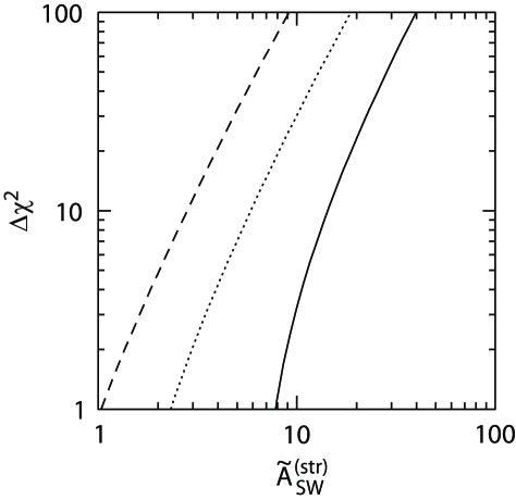
The $\Delta\chi^{2}$ variable for several cases are plotted in Fig. 1. As one can see, $\Delta\chi^{2}_{\rm min}$ drastically increases once $\tilde{A}_{\rm str}$ becomes larger than $O(1-10)$.

From $\Delta\chi^{2}$, we can determine the upper bound on $\tilde{A}^{\rm(str)}_{\rm SW}$. For $\Delta\chi^{2}<4$ ($\Delta\chi^{2}<9$), upper bound on $\tilde{A}^{\rm(str)}_{\rm SW}$ for the flat case (with $l_{\rm max}=300$) and tilted case (with $a_{l<500}=0.2$) is found to be

$$\tilde{A}^{\rm(str)}_{\rm SW}\mathop{}_{\textstyle\sim}^{\textstyle<}\left\{\begin{array}[]{ll}10.6~{}(13.8)&~{}~{}~{}:~{}~{}~{}{\rm flat~{}}(l_{\rm max}=300)\\ 4.0~{}(5.6)&~{}~{}~{}:~{}~{}~{}{\rm tilted~{}}(a_{l<500}=0.2)\end{array}\right..$$ (31)

Since $\Delta\chi^{2}$ drastically increases once $\tilde{A}^{\rm(str)}_{\rm SW}$ becomes larger than $\sim 10$, the above upper bound does not become much larger than $10$ irrespective of the detailed shape of $C_{l}^{\rm(str)}$. For example, for the flat case, $\Delta\chi^{2}<4$ results in $\tilde{A}^{\rm(str)}_{\rm SW}\mathop{}_{\textstyle\sim}^{\textstyle<}7.5$ ($5.1$, $9.1$) for $l_{\rm max}=200$ ($400$, $1000$). Even for $l_{\rm max}=20$, we obtain $\tilde{A}^{\rm(str)}_{\rm SW}\mathop{}_{\textstyle\sim}^{\textstyle<}13.9$. In addition, for the tilted case, we obtain $\tilde{A}^{\rm(str)}_{\rm SW}\mathop{}_{\textstyle\sim}^{\textstyle<}2.6$ and $1.9$ for $a_{l<500}=0.3$ and $0.4$, respectively. Thus, we conclude that $\tilde{A}^{\rm(str)}_{\rm SW}\gg 10$ is highly inconsistent with the observation.

Figure 2: The $\chi^{2}$ variable as a function of $\lambda$ for the flat case with $l_{\rm max}=300$ and $A^{\rm(str)}_{\rm SW}=100$ (solid), $l_{\rm max}=300$ and $A^{\rm(str)}_{\rm SW}=700$ (dotted), and for the tilted case with $a_{l<500}=0.2$ and $A^{\rm(str)}_{\rm SW}=700$ (dashed).

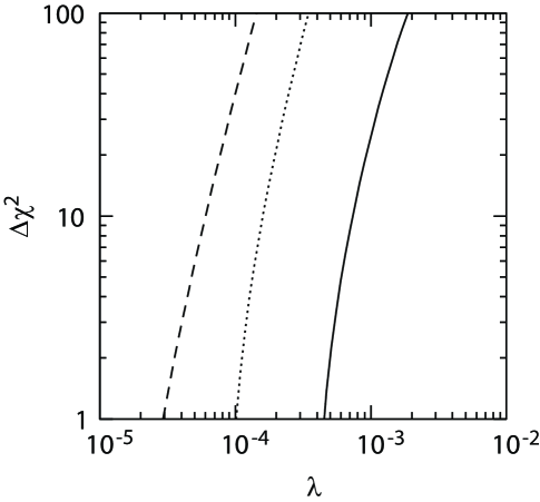
Above upper bounds on $\tilde{A}^{\rm(str)}_{\rm SW}$ are much smaller than the reasonable value of $A^{\rm(str)}_{\rm SW}$ (i.e., $A^{\rm(str)}_{\rm SW}\sim O(100)$). In other words, if we adopt typical value of $A^{\rm(str)}_{\rm SW}$ given in the literatures, $\lambda$ should be sufficiently small to suppress the cosmic-string contribution. In order to derive upper bound on $\lambda$, we calculate the $\chi^{2}$ variable for the flat and tilted cases; we vary $\xi$ to minimize $\chi^{2}$ for fixed value of $\lambda$ and obtain $\chi^{2}_{\rm min}(\lambda)$, the minimum value of $\chi^{2}$ for a fixed value of $\lambda$. In Fig. 2, we plot $\Delta\chi^{2}=\chi^{2}_{\rm min}(\lambda)-\chi^{2}_{\rm min}(\lambda\ll\lambda_{\rm crit})$ as a function of $\lambda$. As one can see, $\lambda$ is required to be smaller than $O(10^{-4}-10^{-5})$. For $\Delta\chi^{2}<4$, the upper bound on $\lambda$ is given by $5.8\times 10^{-4}$ ($1.3\times 10^{-4}$, $4.5\times 10^{-5}$) for the flat case with $l_{\rm max}=300$ and $A^{\rm(str)}_{\rm SW}=100$ (for the flat case with $l_{\rm max}=300$ and $A^{\rm(str)}_{\rm SW}=700$, for the tilted case with $a_{l<500}=0.2$ and $A^{\rm(str)}_{\rm SW}=700$).

If the cosmic-string contribution is negligibly small, the WMAP result can be well described by the $D$-term inflation scenario with ${\cal R}^{\rm(inf)}\simeq 4.5\times 10^{-5}$. Using Eq. (14), we obtain the best-fit value of the $\xi$ as

$$\sqrt{[\xi]_{\rm best}}\simeq 2.6\times 10^{15}\ {\rm GeV}\times\left(\frac{\lambda}{10^{-4}}\right)^{1/3}.$$ (32)

We would like to note here that a consistent scenario of the $D$-term inflation with $\lambda\sim 1$ can be constructed by adopting the curvaton mechanism [10, 11, 12, 13]. In the curvaton scenario, the dominant part of the cosmic density fluctuations are generated from the primordial fluctuation of a late-decaying scalar field $\phi$ (other than inflaton), i.e., so called the curvaton field. The curvaton field $\phi$ has non-vanishing initial amplitude $\phi_{\rm init}$. In addition, the curvaton potential (during inflation) is so flat that $\phi$ acquires quantum fluctuation during inflation:

$$\delta\phi_{\rm init}=\frac{H_{\rm inf}}{2\pi}.$$ (33)

Just after the decay of the inflaton, the curvaton is assumed to be a sub-dominant component of the universe, so the $\delta\phi_{\rm init}$ produces an entropy fluctuation in the curvaton sector. As the universe expands, however, the curvaton dominates the energy density of the universe and then decays to reheat the universe. Important point is that the primordial fluctuation $\delta\phi_{\rm init}$ is converted to purely adiabatic density fluctuations (as far as all the components in the universe, i.e., the baryon, the cold dark matter, and so on as well as the radiation are generated from the decay product of the curvaton). Since $H_{\rm inf}$ does not change much during the $D$-term inflation, (almost) scale-invariant adiabatic cosmic density fluctuations can be realized if the curvaton contribution is large enough. Effect of $\delta\phi_{\rm init}$ on the CMB anisotropy is parameterized by a single parameter, which we choose to be the metric perturbation (in the RD epoch after the decay of the curvaton field) induced by the curvaton fluctuation [11, 12]:

$$\Psi^{\rm(curv)}_{\rm RD}=-\frac{4}{9}\frac{\delta\phi_{\rm init}}{\phi_{\rm init}}=-\frac{2}{9\sqrt{6}\pi}\frac{g\xi}{M_{*}\phi_{\rm init}}.$$ (34)

Since there is no correlation between the primordial fluctuations in the inflaton and curvaton fields, the total CMB angular power spectrum is now given in the form

$$C_{l}=C_{l}^{\rm(inf)}+C_{l}^{\rm(str)}+C_{l}^{\rm(curv)},$$ (35)

where $C_{l}^{\rm(curv)}$ is the curvaton contribution. As we emphasized, the density fluctuations associated with $\delta\phi_{\rm init}$ is purely adiabatic. In addition, $\Psi^{\rm(curv)}$ is almost scale-invariant since the expansion rate during the $D$-term inflation is almost constant. As a result, the total CMB angular power spectrum may become well consistent with the WMAP observation if the curvaton contribution dominates over the inflaton contribution. We can see that such a hierarchy is relatively easily realized; using the fact that $C_{l}^{\rm(inf)}$ and $C_{l}^{\rm(str)}$ are proportional to $[\Psi^{\rm(inf)}]^{2}\propto\mu^{2}$ when $\lambda\sim 1$ while $C_{l}^{\rm(curv)}$ is proportional to $[\Psi^{\rm(curv)}]^{2}$, the curvaton contribution dominates when $\phi_{\rm init}\mathop{}_{\textstyle\sim}^{\textstyle<}gM_{*}$ since $\Psi^{\rm(inf)}\sim O(\xi/M_{*}^{2})$.

To be more quantitative, we calculate the $\chi^{2}$ variable to derive constraints on the parameters in the scenario. Now the total angular power spectrum has the form

$$C_{l}=[C_{l}^{\rm(adi)}]_{\Psi_{\rm RD}=1}\Psi_{\rm RD}^{2}+[C_{l}^{\rm(str)}]_{G\mu=1}(G\mu)^{2},$$ (36)

where

$$\Psi_{\rm RD}^{2}=[\Psi^{\rm(inf)}_{\rm RD}]^{2}+[\Psi^{\rm(curv)}_{\rm RD}]^{2},$$ (37)

and $C_{l}^{\rm(adi)}$ is the CMB angular power spectrum generated from purely adiabatic density fluctuations. Then, as we discussed in the case without the curvaton, the $\chi^{2}$ variable is minimized when the cosmic-string contribution is negligibly small and $\Psi_{\rm RD}\simeq 3.0\times 10^{-5}$. The latter condition can be satisfied by tuning the curvaton contribution (as far as the inflaton contribution to $\Psi_{\rm RD}$ is not too large.) In order to realize hierarchy between the adiabatic and cosmic-string contributions, it is necessary to make $\mu$ small by suppressing $\xi$. Requiring that $\Delta\chi^{2}<4$, we obtain the upper bound on $\mu$ for the case of $\lambda\sim 1$ as

$$A^{\rm(str)}_{\rm SW}\times(G\mu/10^{-6})^{2}\mathop{}_{\textstyle\sim}^{\textstyle<}\left\{\begin{array}[]{ll}80&~{}~{}~{}:~{}~{}~{}{\rm flat~{}}(l_{\rm max}=300)\\ 30&~{}~{}~{}:~{}~{}~{}{\rm tilted~{}}(a_{l<500}=0.2)\end{array}\right.,$$ (40)

and hence, using Eq. (16), the upper bound on $\xi$ is given by

$$\sqrt{\xi}/M_{*}\mathop{}_{\textstyle\sim}^{\textstyle<}(A^{\rm(str)}_{\rm SW}/100)^{-1/4}\times\left\{\begin{array}[]{ll}1.9\times 10^{-3}&~{}~{}~{}:~{}~{}~{}{\rm flat~{}}(l_{\rm max}=300)\\ 1.5\times 10^{-3}&~{}~{}~{}:~{}~{}~{}{\rm tilted~{}}(a_{l<500}=0.2)\end{array}\right..$$ (43)

In addition, using the best-fit value of $\Psi_{\rm RD}$ given above, we can estimate the required value of the initial amplitude of the curvaton field. Importantly, in order to realize the adiabatic-like CMB angular power spectrum, $\Psi^{\rm(curv)}\gg\Psi^{\rm(inf)}$ since $C_{l}^{\rm(str)}$ and $C_{l}^{\rm(inf)}$ are of the same order if $\lambda\sim 1$. Thus, requiring $\Psi^{\rm(curv)}_{\rm RD}\simeq 3.0\times 10^{-5}$, we obtain

$$\phi_{\rm init}/M_{*}\simeq 9.5\times 10^{2}\times g\left(\frac{\sqrt{\xi}}{M_{*}}\right)^{2}.$$ (44)

We should also note here that, in the $D$-term inflation scenario, Hubble-induced mass term of the scalar fields does not exist. This fact has an important implication to the curvaton scenario. The curvaton field should acquire sizable primordial quantum fluctuation. Thus, the curvaton potential should be sufficiently flat during inflation, which is naturally realized in the $D$-term inflation. In models where the vacuum energy during the inflation is from $F$-term interaction, however, it is non-trivial to realize the flatness of the curvaton potential during the inflation. Thus, the $D$-term inflation provides a consistent scenario of the curvaton paradigm.

Finally, we would like to make a brief comment on the cases of hybrid inflation. In many classes of hybrid inflation models, gauged U(1) symmetry exists which is spontaneously broken after the inflation. With such a U(1) symmetry, cosmic string is also formed, which also affects the CMB anisotropy. The dynamics of the hybrid inflation and the mass of the string per unit length are almost the same as the D-term inflation [34]. Therefore, the result obtained in the present work can apply to the hybrid inflation. Of course, for general hybrid inflation models where the cosmic string affects the CMB anisotropy too much to be consistent with the observations, the curvaton mechanism can solve the difficulty as in the $D$-term inflation case.

References

- [1] A.H. Guth, Phys. Rev. D23 (1981) 347.
- [2] K. Sato, MNRAS 195 (1981) 467.
- [3] E. Haylo, Phys. Lett. B387 (1996) 43.
- [4] P. Binetruy and G. Dvali, Phys. Lett. B388 (1996) 241.
- [5] R. Jeannerot, Phys. Rev. D56 (1997) 6205.
- [6] D.H. Lyth and A. Riotto, Phys. Lett. B412 (1997) 28.
- [7] N. Kaiser and A. Stebbins, Nature 310 (1984) 391.
- [8] J.R. Gott, Astrophys. J. 288 (1985) 422.
- [9] G. Hinshaw et al., astro-ph/0302217.
- [10] D.H. Lyth and D. Wands, Phys. Lett. B524 (2002) 5.
- [11] T. Moroi and T. Takahashi, Phys. Lett. B522 (2001) 215.
- [12] T. Moroi and T. Takahashi, Phys. Rev. D66 (2002) 063501.
- [13] D.H. Lyth, C. Ungarelli and D. Wands, Phys. Rev. D67 (2003) 023503.
- [14] G. Veneziano, Phys. Lett. B265 (1991) 287.
- [15] M. Gasperini and G. Veneziano, Astropart. Phys. 1 (1992) 1.
- [16] M. Gasperini and G. Veneziano, Phys. Rev. D50 (1994) 2519.
- [17] J. Khoury, B.A. Ovrut, P.J. Steinhardt and N. Turok, Phys. Rev. D64 (2001) 123522.
- [18] J. Khoury, B.A. Ovrut, N. Seiberg, P.J. Steinhardt and N. Turok, Phys. Rev. D65 (2002) 086007.
- [19] J. Khoury, B.A. Ovrut, P.J. Steinhardt and N. Turok, Phys. Rev. D66 (2002) 046005.
- [20] K. Enqvist and M.S. Sloth, Nucl. Phys. B626 (2002) 395.
- [21] J.M. Bardeen, P.J. Steinhardt and M.S. Turner, Phys. Rev. D28 (1983) 629.
- [22] W. Hu, Ph.D thesis (astro-ph/9508126).
- [23] M. Zaldarriaga and U. Seljak, Astrophys. J. 469 (1996) 437.
- [24] D.N. Spergel et al., astro-ph/0302209.
- [25] See, for example, A. Vilenkin and E.P.S. Shellard, “Cosmic Strings and Other Topological Defects” (Cambridge University Press, 1994).
- [26] B. Allen, R.R. Caldwell, E.P.S. Shellard, A. Stebbins and S.Veeraraghavan, Phys. Rev. Lett. 77 (1996) 3061.
- [27] B. Allen, R.R. Caldwell, S. Dodelson, L. Knox, E.P.S. Shellard and A. Stebbins, Phys. Rev. Lett. 79 (1997) 2624.
- [28] M. Landriau, E.P.S. Shellard, astro-ph/0302166.
- [29] C.R. Contaldi, M. Hindmarsh and J. Magueijo, Phys. Rev. Lett. 82 (1999) 679.
- [30] A. Albrecht, R.A. Battye and J. Robinson, Phys. Rev. D59 (1999) 023508.
- [31] L.Pogosian and T.Vachaspati, Phys. Rev. D60 (1999) 083504.
- [32] E.J. Copeland, J. Magueijo and D.A.Steer, Phys. Rev. D61 (2000) 063505.
- [33] L. Verde et al., astro-ph/0302218.
- [34] T. Asaka, K. Hamaguchi, M. Kawasaki and T. Yanagida, Phys. Rev. D61 (2000) 083512.