Fermions in the vortex background on a sphere

Abstract:

In 5+1 dimensions, we construct a vortex-like solution on a two-dimensional sphere. We study fermionic zero modes in the background of this solution and relate them to the replication of fermion families in the Standard Model. In particular, using a compactified space removes the need for the difficult localisation of gauge fields, while the present procedure (rather than naive compactification on a disk) also removes spurious fermionic modes.

1 Introduction.

Coupling of fermions to background bosonic fields of nontrivial topology may lead to chiral fermionic zero modes. In particular, for the case of the Abrikosov-Nielsen-Olesen vortex this fact is widely known for several decades [1]. The number of the zero modes coincides with the topological number, that is, with the magnetic flux of the vortex. One remarkable application of this feature is to models with Large Extra Dimensions (LED) where chiral fermions of the Standard Model are described by the zero modes of multi-dimensional fermions localized in the (four-dimensional) core of a topological defect [2]. In particular, this approach can explain the origin of the fermionic family replication and the fermionic mass hierarchy. In Refs. [3, 4, 5, 6], we have constructed and studied models in which a single family of fermions in six dimensions with vector-like couplings to the Standard Model (SM) bosons gives rise to three generations of chiral Standard Model fermions in four dimensions. We have also shown that in these models a power-like hierarchy of the fermionic masses and mixings appears in a natural way.

One of the principal issues of models with LED is the localization of the Standard Model gauge fields. One of possible ways to avoid this problem is to consider the transverse extra dimensional space as a compact manifold and to allow gauge fields to propagate freely in the extra dimensions. It is however not a straightforward task to put a vortex and fermionic zero modes in a finite volume space. Indeed, in a flat space with a boundary, ”stray” fermionic zero modes of opposite chirality appear in addition to the chiral zero modes localized in the core. This happens because of the finite volume of the bulk: the modes which would have been killed by the normalization condition in the case of infinite space, survive in a finite volume. Even imposing the physical boundary condition which corresponds to the absence of the fermionic current outside the boundary does not help since the current of the zero modes lack radial components. Another approach to the localization of gauge fields in the vortex background is also possible. In particular, in [7, 8] a vortex-like solution was considered in the presence of gravity. It was shown that the localized zero modes of vector field appear in these models.

In this paper we consider the vortex and the fermions taking a two dimensional sphere as extra dimensions. Keeping in mind the application of this system to the model with LED we will refer to the coordinates on the sphere as to the fourth and the fifth coordinates on this $M^{4}\times S^{2}$ manifold, where $M^{4}$ represents our four-dimensional Minkowski space. Our results, however, do not depend on the number of ordinary dimensions. We will argue also that the main features of the ”flat” models  [3, 4, 5, 6] remain intact in the spherical case.

2 Vortex on a sphere.

In this section we construct the Abrikosov-Nielsen-Olesen vortex solution on a $M^{4}\times S^{2}$ manifold. The metric $g_{AB}$ of this manifold is determined by

$$ds^{2}=g_{AB}dx^{A}dx^{B}=g_{\mu\nu}dx^{\mu}dx^{\nu}-R^{2}(d\theta^{2}+\sin^{2}\theta d\varphi^{2}),$$ (1)

where $g_{\mu\nu}={\rm diag}(+,-,\ldots,-)$ is the four dimensional Minkowski metric, capital Latin indices are $A,B=0,\ldots 5$, Greek indices are $\mu,\nu=0,\ldots,3$. To generate the vortex solution we introduce an Abelian Higgs Lagrangian,

$${\cal L}_{V}=\sqrt{-\det(g_{AB})}\left(-\frac{1}{4}F_{AB}F^{AB}+(D^{A}\Phi)^{\dagger}D_{A}\Phi-\frac{\lambda}{2}(|\Phi|^{2}-v^{2})^{2}\right),$$ (2)

where $F_{AB}=\partial_{A}A_{B}-\partial_{B}A_{A}$, $D_{A}\Phi=(\partial_{A}-ieA_{A})\Phi$, $A_{A}$ and $\Phi$ are a $U(1)$ gauge field and a complex scalar field, respectively.

The vortex solution which we are interested in is a static solution of the field equations depenging only on $\theta$ and $\varphi$, the coordinates on $S^{2}$. Let us introduce the standard ansatz for a vortex with winding number one,

$$A_{\varphi}=\frac{1}{e}A(\theta)\,,\ \ \ A_{\theta}=0\,,\ \ \ \Phi=F(\theta){\rm e}^{i\varphi}.$$ (3)

We obtain the following set of the field equations,

$$\frac{1}{\sin{\theta}}\partial_{\theta}\frac{1}{\sin{\theta}}\partial_{\theta}A-\frac{2R^{2}e^{2}}{\sin^{2}{\theta}}F^{2}(A-1)=0,$$ (4)

$$\frac{1}{\sin{\theta}}\partial_{\theta}\sin{\theta}\partial_{\theta}F-\frac{1}{\sin^{2}{\theta}}F(A-1)^{2}-\lambda R^{2}F(F^{2}-v^{2})=0.$$ (5)

Let us discuss now the boundary conditions to the field equations. To obtain a non-trivial soliton one should impose zero boundary conditions for the fields $A(\theta)$ and $F(\theta)$ on the North pole of the sphere ($\theta=0$) and non-zero boundary conditions on the South pole of the sphere ($\theta=\pi$). However, the ansatz (3) with these boundary conditions is singular on the South pole due to the $\varphi$-dependence. To avoid this difficulty we essentially repeat the discourses by Wu and Yang [9]. We introduce two patches on the sphere and a different ansatz in the Southern patch,

$$A_{\varphi}^{S}=\frac{1}{e}A^{S}(\theta)\,,\ \ \ A_{\theta}^{S}=0\,,\ \ \ \Phi=F^{S}(\theta),$$ (6)

where

$$A^{S}(\pi)=0\,,\ \ \ \partial_{\theta}F(\pi)=0.$$ (7)

In the overlapping region the two ansatzes (3) and (6) are related by a gauge transformation:

$$F(\theta){\rm e}^{i\varphi}={\rm e}^{i\alpha}F^{S}(\theta),$$ (8)

$$A(\theta)=A^{S}(\theta)+\partial_{\varphi}\alpha.$$

Therefore, to satisfy the first of the equations one can choose $\alpha=\varphi$ and, hence,

$$A(\theta)=A^{S}(\theta)+1.$$ (9)

If one introduces now another field $\Psi$ coupled to $A_{A}$ with the charge $q$, thus transforming as

$$\Psi^{\prime}=\Omega\Psi=\exp\left(i\frac{q}{e}\alpha\right)\Psi,$$

then one should require $\Omega$ to be single-valued which brings in turn the famous Dirac’s quantization condition

$$\frac{q}{e}=\mbox{integer}$$ (10)

This situation differs from the flat case where one might introduce fields with the half-integer charge.

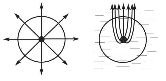
The necessity of the two patches and the appearance of the Dirac’s condition become more transparent if we examine the following relationship between the vortex on $S^{2}$ and a monopole in the three dimensional space. Let us consider a monopole with the magnetic charge $g_{M}$ in three dimensions in vacuum. The field configuration of the monopole is spherically symmetric as it is shown on the left hand side of the Fig. 1. If we now place the monopole in the superconducting medium, then the magnetic field would be pushed out and spherical symmetry would break down as is depicted on the right hand side of the Fig. 1. The region where the magnetic lines cross a sphere surrounding the monopole will be nothing else than a core of a vortex on this sphere. The magnetic flux through the sphere is $4\pi g_{M}$. From the other hand, the magnetic flux calculated on the solutions (3) and (6) is $2\pi/e$. Comparing these two fluxes one finds $e=1/(2g_{M})$, that is $e$ is the minimal quantum of charge in a full agreement with Eq. (10).

Let us note that spontaneous compactification on a monopole configuration is well-known in Kaluza-Klein models (see, for instance, Refs. [10]). There, fermionic zero modes appear which are not localized at any particular point of the sphere. Our approach with a vortex allows one to use a similar mechanism in LED models and to study the hierarchy of the fermion masses.

Figure 1: A monopole in the vacuum (left) and in the superconducting medium (right).

As we have seen, to describe the vortex configuration on $S^{2}$ it is necessary to introduce two patches on the sphere. In practical calculations it is more convenient, however, to deal with the singular ansatz (3). To achieve this, one may send the size of the Southern patch to zero and essentially introduce the Dirac string. In that case one obtains from Eqs. (7), (8), (9) the following boundary conditions:

$$A(\pi)=1\,,\ \ \ \ \partial_{\theta}F(\pi)=0.$$ (11)

Solving the equations (4), (5) with these boundary conditions one finds the behaviour of $A$ and $F$ near the North and the South poles ($\xi=\pi-\theta$):

$$A(\theta)=C_{0A}\theta^{2}\,,\ \ \ \ F(\theta)=C_{0F}\theta\ \ \mbox{at}\ \ \theta\to 0;$$ (12)

$$A(\xi)=1-C_{\pi A}\xi^{2}\,,\ \ \ \ F(\xi)=C_{\pi F}\left(1-\lambda\frac{v^{2}-C_{\pi F}^{2}}{4}\xi^{2}\right)\ \ \mbox{at}\ \ \theta\to\pi,$$ (13)

where $C_{0A}$, $C_{0F}$, $C_{\pi A}$, and $C_{\pi F}$ are unknown constants ($C_{\pi F}<v$). Note that the number of the unknown constants is enough to match the solutions (12), (13) at some interior point. This in turn is a strong argument that the solution to Eqs. (4), (5) with boundary conditions (11) does exist.

To complete this section we note that, in the spirit of the Witten’s work [11], a scalar field can be introduced which has a non-zero value near the North pole and vanishes at the South pole. This Higgs field is required in the LED models [3] to give masses to fermionic zero modes. The lagrangian of this field is

$${\cal L}_{H}=\sqrt{-\det(g_{AB})}\left((D^{A}H)^{\dagger}D_{A}H-\frac{\kappa}{2}(|H|^{2}-\mu^{2})^{2}-h^{2}|H|^{2}|\Phi|^{2}\right),$$

where $D_{A}H=(\partial_{A}+ieA_{A})H$. Making use of the arguments of Ref. [11], one can show that with $h^{2}v^{2}>\kappa\mu^{2}$, there is a stable solution to the field equations $H(\theta)$ which depends only on $\theta$. This solution is non-zero at the North pole, $0<H(0)<\mu$, and is zero at the South pole, $H(\xi)=C_{\pi H}\xi^{2}$ at $\theta\to\pi$. The typical size of the solution is of order of the typical size of the field $\Phi$ (for details, see Ref. [6] where the flat case is discussed).

3 Fermionic zero modes in the vortex background.

In this section we consider fermions and their zero modes in the vortex background on $S^{2}$. As in the previous section, we work on $M^{4}\times S^{2}$ manifold. Fermions on this manifold may be represented by eight-component spinors. We use the chiral representation for the six-dimensional flat Dirac $\Gamma$-matrices (see Ref. [3] for notations). In particular, $\Gamma_{7}={\rm diag}({\bf 1},{\bf-1})$ is a six-dimensional analog of the four-dimensional $\gamma_{5}$.

In the case of the flat space, to obtain fermionic zero modes one usually considers fermions with a half-integer axial charge with respect to the vortex group:

$$\Psi^{\prime}={\rm e}^{i\frac{\Gamma_{7}}{2}\alpha}\Psi.$$ (14)

However, as we have seen in the previous section, in the case of the vortex on a sphere it is inconsistent to introduce fields with the half-integer charge. To avoid this difficulty, we change the representation (14) and consider fermions transforming as

$$\Psi^{\prime}={\rm e}^{i\frac{(1+\Gamma_{7})}{2}k\alpha}\Psi,$$ (15)

where $k$ is a positive integer number. Then, both Weyl spinors which comprise the Dirac spinor $\Psi$, have integer charges in agreement with Eq. (10). In what follows, we will demonstrate that there are exactly $k$ chiral (from the four-dimensional point of view) fermionic zero modes.

To describe fermions on $M^{4}\times S^{2}$ manifold with the metric (1) we introduce the following sechsbein,

$$h^{a}_{A}=(\delta^{a}_{\mu},\,\delta^{a}_{4}R,\,\delta^{a}_{5}R\sin\theta),$$ (16)

where lower case Latin indices $a,b=0,\ldots,5$ correspond to the flat tangent six-dimensional Minkowski space. Then the covariant (with respect to general coordinate transformations) derivative,

$$\nabla_{A}\Psi=\left(\partial_{A}+\frac{1}{4}R_{A}^{ab}\Gamma_{b}\Gamma_{a}\right),$$

where the spin connection is defined as

$$R_{A}^{ab}=(\nabla_{A}h^{Ba})h^{b}_{B},$$

has only one non-trivial component,

$$\nabla_{\varphi}=\partial_{\varphi}+\frac{\cos\theta}{2}\Gamma^{4}\Gamma^{5}.$$

All other components coincide with the usual derivatives.

The lagrangian of the fermions which is invariant under both gauge (15) and general coordinate transformations may be chosen as

$${\cal L}_{\Psi}=\sqrt{-\det(g_{AB})}\left\{i\bar{\Psi}h^{A}_{a}\Gamma^{a}\!\left(\!\nabla_{A}-iek\frac{1+\Gamma_{7}}{2}A_{A}\!\right)\!\Psi-g\Phi^{k}\bar{\Psi}\frac{1-\Gamma_{7}}{2}\Psi-g\Phi^{*k}\bar{\Psi}\frac{1+\Gamma_{7}}{2}\Psi\right\}.$$ (17)

We apply now the standard decomposition procedure. Since the vortex background does not depend on $x_{\mu}$, one can separate variables related to $M^{4}$ and $S^{2}$. To this end let us introduce the transverse Dirac operator in the background (3),

$$D=\frac{\Gamma^{0}}{R}\left\{i\Gamma^{4}\partial_{\theta}+i\frac{\Gamma^{5}}{\sin\theta}\left(\partial_{\varphi}+\frac{\cos\theta}{2}\Gamma^{4}\Gamma^{5}-ik\frac{1+\Gamma_{7}}{2}A\right)-gR\Phi^{k}\frac{1-\Gamma_{7}}{2}-gR\Phi^{*k}\frac{1+\Gamma_{7}}{2}\right\},$$

and expand any spinor in a set of the eigenvectors $\Psi_{m}$ of this operator

$$D\Psi_{m}=m\Psi_{m}$$

There may exist a set of discrete eigenvalues $m$ with the separation of order $gv^{k}$, and the continuous spectrum starting from $m\gtrsim gv^{k}$. All these eigenvalues play a role of the mass of the corresponding four-dimensional excitations (see Ref. [3] for details). In what follows we assume that the energy scales probed by a four-dimensional observer are smaller than $gv^{k}$, and thus even the first non-zero level is not excited. So, we are interested only in the zero modes of $D$:

$$D\Psi=0.$$ (18)

To solve the equation (18), we first of all separate $\phi$ and $\theta$-dependence. The operator of the generalized angular momentum (see, for instance, Ref. [12]) commuting with $D$ is, in our case,

$$J=-i\partial_{\varphi}-k\frac{1+\Gamma_{7}}{2}.$$

The eigenvectors of this operator with the antiperiodic boundary conditions are

$$\Psi_{n}(\theta,\varphi)=\exp\left[i\varphi\left(k\frac{1+\Gamma_{7}}{2}-n+\frac{1}{2}\right)\right]\Psi(\theta,n)=\left(\begin{array}[]{l}{\bf 1}\cdot{\rm e}^{i\varphi\frac{2k-2n+1}{2}}f_{1}(\theta)\\ {\bf 1}\cdot{\rm e}^{i\varphi\frac{2k-2n+1}{2}}f_{2}(\theta)\\ {\bf 1}\cdot{\rm e}^{-i\varphi\frac{2n-1}{2}}f_{3}(\theta)\\ {\bf 1}\cdot{\rm e}^{-i\varphi\frac{2n-1}{2}}f_{4}(\theta)\\ \end{array}\right),$$ (19)

where $n$ is an integer number and ${\bf 1}=(1,1)^{T}$ is a two component spinor.

Substituting Eq. (19) into Eq. (18), one obtains the following two sets of the differential equations,

$$\left\{\begin{array}[]{l}\left[\partial_{\theta}+\displaystyle\frac{\cot\theta}{2}-\frac{1}{\sin\theta}\left(n-\frac{1}{2}-k(1-A)\right)\right]f_{1}-Qf_{4}=0,\\ \\ \left[\partial_{\theta}+\displaystyle\frac{\cot\theta}{2}+\frac{1}{\sin\theta}\left(n-\frac{1}{2}\right)\right]f_{4}-Qf_{1}=0;\end{array}\right.$$ (20)

$$\left\{\begin{array}[]{l}\left[\partial_{\theta}+\displaystyle\frac{\cot\theta}{2}+\frac{1}{\sin\theta}\left(n-\frac{1}{2}-k(1-A)\right)\right]f_{2}+Qf_{3}=0,\\ \\ \left[\partial_{\theta}+\displaystyle\frac{\cot\theta}{2}-\frac{1}{\sin\theta}\left(n-\frac{1}{2}\right)\right]f_{3}+Qf_{2}=0,\end{array}\right.$$ (21)

where

$$Q(\theta)=gRF^{k}(\theta).$$ (22)

Note that the equations (20) can be obtained from the equations (21) by the replacement $n-1\to-n$, $k\to-k$, $Q\to-Q$, $f_{2}\to f_{1}$, $f_{3}\to f_{4}$.

Let us consider the equations (21) for $f_{2,3}$. It is convenient to introduce new functions $g_{2,3}$ defined by

$$f_{2,3}=g_{2,3}\frac{\sin^{(k-n)}\frac{\theta}{2}}{\cos^{(k-n+1)}\frac{\theta}{2}}\exp\left(-k\int\limits^{\theta}\frac{A(x)}{\sin x}dx\right).$$ (23)

Then the equations for $g_{2,3}$ take the following form (the prime denotes a derivative with respect to $\theta$):

$$g^{\prime\prime}_{2}-\left[\frac{Q^{\prime}}{Q}+\frac{1}{\sin\theta}(2n-1-k(1-A))\right]g^{\prime}_{2}-Q^{2}g_{2}=0,$$ (24)

$$g_{3}=-\frac{g^{\prime}_{2}}{Q}.$$ (25)

To proceed further, we will need the following theorem.

Theorem 1

Let $g_{2}$ satisfy the Eq. (24) with $Q$ which is differentiable and has no nodes at the interior points of the interval $0<\theta<\pi$ and $A$ which has no singularities. Assume that at some interior point $\theta_{0}$, $g_{2}$ and $g_{2}^{\prime}$ have the same sign. Then $g_{2}$ and $g_{2}^{\prime}$ have the same sign at all points $\theta_{0}<\theta<\pi$.

Proof. To prove the theorem, one notes that if a function and its derivative at some point have the positive (negative) sign then at this point the function grows (falls). This means that the (continuous) function cannot change its sign before its derivative does it. Let us assume that there is a point $\pi>\theta_{m}>\theta_{0}$ in which the derivative changes its sign. This point is nothing else than a local maximum (minimum) of the function. Since we have supposed that $Q^{\prime}/Q$ and $A$ are regular (which is true for the vortex background), the coefficient before the second term in (24) is non-singular at $\theta_{m}$ and hence this term vanishes at $\theta_{m}$. Due to Eq. (24), this means that the second derivative is strictly positive (negative) at $\theta_{m}$ which is in contradiction with the statement that this point is a maximum (minimum). Thus we have shown the validity of Theorem 1.

It follows trivially from the theorem that if $g_{2}$ and its derivative have different signs at some point $\theta_{0}$, then they have different signs at all points $0<\theta<\theta_{0}$.

Now we are ready to demonstrate that the equations (21) possess exactly $k$ normalizable solutions (at $k>0$) while Eqs. (20) have no normalizable solution. Consider first the case $n>0$.

(i) Let us find the behaviour of $g_{2}$ in the vicinity of the South pole ($\xi=\pi-\theta$, $\xi\to 0$). Near the South pole $Q^{\prime}\to 0$, $A\to 1$. So, Eq. (24) has two linearly independent solutions,

$$g_{2\pi}^{(1)}=a_{\pi}\left(1+\frac{Q_{\pi}}{4n}\xi^{2}+\ldots\right)$$ (26)

and

$$g_{2\pi}^{(2)}=b_{\pi}\xi^{2-2n}(1+\ldots),$$

where $a_{\pi}$ and $b_{\pi}$ are unknown constants, $Q_{\pi}\equiv Q(\pi)$. (For $n=1$, $g_{2\pi}^{(2)}=b_{\pi}\ln\xi$.) The function $g_{2\pi}^{(2)}$ yields the following behaviour of $f_{3}$,

$$f_{3\pi}^{(2)}\sim\frac{b_{\pi}}{\xi^{n}},$$

which is not normalizable at $n>0$. We conclude that $b_{\pi}=0$. Thus,

$$f_{2\pi}\sim a_{\pi}\xi^{n-1}\,,\ \ \ f_{3\pi}\sim a_{\pi}\xi^{n}.$$

(ii) Since only one solution $g_{2\pi}^{(1)}$, Eq. (26), survives at the South pole, we are able to determine the relative sign of the function $g_{2}$ and its derivative. Indeed, it follows from Eq. (26) that $g_{2}$ and $g_{2}^{\prime}$ have different signs near the South pole. Due to Theorem 1 this means that $g_{2}$ and $g_{2}^{\prime}$ have different signs in the whole interval $0<\theta<\pi$.

(iii) Let us investigate now the behaviour of $g_{2}$ in the vicinity of the North pole ($\theta\to 0$). There (see Eqs. (22), (12)), $Q=C_{Q}\theta^{k}$ and $A=C_{0A}\theta^{2}$, where $C_{Q}=gRC_{0F}^{k}$. Two linearly independent solutions of Eq.(24) are

$$g_{20}^{(1)}=a_{0}\left(1+\frac{C_{Q}^{2}}{4(k+1)(k+1-n)}\theta^{2k+2}+\ldots\right)$$ (27)

and

$$g_{20}^{(2)}=b_{0}\theta^{2n}\left(1+{\cal O}(\theta^{2})\right),$$

where $a_{0}$ and $b_{0}$ are some unknown constants.

Note that for $n>0$, $g_{20}^{(2)}$ and its derivative have the same sign at $\theta\to 0$. So, we conclude that in order to satisfy the (ii) condition, $a_{0}$ could not be zero. From the other hand, it follows from Eqs. (27) and (23) that

$$f_{20}^{(1)}\sim a_{0}\theta^{k-n}.$$

Therefore, $f_{2}$ can be normalized iff $k\geq n$. If the latter condition holds, then $g_{20}^{(1)}$ and its derivative have the same sign. Again, to satisfy the (ii) condition, $b_{0}$ should be non-zero. Thus, at $\theta\to 0$ the normalizable solution of (24) is

$$g_{20}=g_{20}^{(1)}+g_{20}^{(2)}$$ (28)

with non-zero $a_{0}$ and $b_{0}$. Using Eqs. (28), (25), and (23) we obtaine the following behaviour of $f_{2,3}$ at small $\theta$:

$$f_{2}\sim a_{0}\theta^{k-n},$$ (29)

$$f_{3}\sim b_{0}\theta^{n-1}$$ (30)

for $0<n\leq k$ which corresponds to exactly $k$ normalizable modes.

The case $n\leq 0$ as well as Eq. (20) can be considered in a similar way. Namely, one should find the behaviour of $g_{2}$ ($g_{1}$) at the South pole and make sure that only one solution survives, then check that this solution and its derivative have different signs near the South pole. Theorem 1 then implies that the solution and its derivative have different signs at all points. Then one finds the behaviour of the solution in the vicinity of the North pole, makes sure that both linearly independent solutions should contribute in order to satisfy the ”different sign condition”, and checks that there is no $n$ at which the solution is not singular at the North pole.

To conclude this section let us give four notes in turn. First, we have obtained exactly $k$ modes with non-vanishing $f_{2}$ and $f_{3}$ and vanishing $f_{1}$ and $f_{4}$. These modes are all left handed from the four-dimensional point of view (for the discussion, see Ref. [3]). The theory with the Lagrangian (17) in the presence of other gauge fields is anomalous however (see also Ref. [8] for a discussion).

. In order to obtain right handed modes and to make the theory anomaly free, one introduces other spinors which rotate under the (vortex) gauge transformations as

$$\Upsilon^{\prime}={\rm e}^{i\frac{1-\Gamma_{7}}{2}k\alpha}\Upsilon.$$ (31)

In that case one finds the following zero modes,

$$\Upsilon_{n}(\theta,\varphi)=\left(\begin{array}[]{l}{\bf 1}\cdot{\rm e}^{-i\varphi\frac{2n-1}{2}}f_{3}(\theta,g_{\Upsilon})\\ 0\\ 0\\ {\bf 1}\cdot{\rm e}^{i\varphi\frac{2k-2n+1}{2}}f_{2}(\theta,g_{\Upsilon})\\ \end{array}\right)$$ (32)

where the functions $f_{2}$ and $f_{3}$ satisfy Eqs. (21) with a new Yukawa coupling $g_{\Upsilon}$.

Second, one can also obtain left- and right-handed modes by introducing spinors with the charges $ke(-1+\Gamma_{7})/2$ and $-ke(1+\Gamma_{7})/2$ (instead of (15) and (31)), respectively. The new zero mode can be obtained from (19) and (32) by means of $CP$-conjugation; for instance, the new right-handed mode is $\Gamma_{0}\Gamma_{2}\Gamma_{4}\Upsilon^{*}$. For the given Yukawa couplings in (34) this choice actually leads to a different mass spectrum which we do not consider here.

Third, to localize $k$ modes we have used the vortex with the winding number one and somewhat unusual Yukawa coupling in Eq. (17). However, nothing changes in this construction if one considers the vortex with the winding number $k$ and fermions with charge $e(1+\Gamma_{7})/2$. Then one would have a usual Yukawa term $\Phi\bar{\Psi}(1-\Gamma_{7})\Psi$.

Fourth, we have found the behaviour of the zero modes (29), (30) up to unknown constants $a_{0}$ and $b_{0}$. These constants are important for the LED models if the Standard Model fermionic mass pattern is to be determined. To find $a_{0}$ and $b_{0}$ one should use the normalization condition which reads as

$$1=2\pi R^{2}\int\limits_{0}^{\pi}\!d\theta\sin\theta(f_{2}^{2}+f_{3}^{2}).$$ (33)

In the next section, we will estimate $a_{0}$ and $b_{0}$ and demonstrate that the mass hierarchy is indeed reproduced in this model.

4 Mass hierarchy.

In the previous section, we have found $k$ chiral fermionic zero modes in the vortex background on a sphere. In the LED models [4] these modes are interpreted as the Standard Model fermions. In particular, at $k=3$ we obtain three generations of the fermions. These fermions get their masses and mixings from the Yukawa interaction,

$$HX\bar{\Psi}\frac{1-\Gamma_{7}}{2}\Upsilon+\epsilon H\Phi\bar{\Psi}\frac{1-\Gamma_{7}}{2}\Upsilon,$$ (34)

where $H$ is the Standard Model Higgs boson which has a non-trivial profile on the sphere (see the end of Section 2), $X$ is an additional scalar which also has a non-trivial profile similar to the one of $H$, and $\epsilon$ is a small constant (see Refs. [4, 6] for details). In this section, we demonstrate that the hierarchical mass pattern inherent to the flat-space construction of Ref. [4] is reproduced in the spherical case. For the sake of example we just discuss the case of the diagonal masses which appear after the integration over the sphere from the first term in Eq. (34) (we assume that $g=g_{\Upsilon}$ for simplicity),

$$m_{nn}\sim\int\limits_{0}^{\pi}\!d\theta\sin\theta H(\theta)X(\theta)f_{2}^{2}(n,\theta).$$ (35)

The mixings appear from the second term and can be easily treated in a similar way.

Let $R\theta_{\Phi}\sim 1/\sqrt{\lambda}v$ be the typical size of $\Phi$. Then, as it has been pointed out in the Section 2, the typical width of $H$ is also of order $R\theta_{\Phi}$. The integral in Eq. (35) saturates in the region $0<\theta<\theta_{\Phi}$. In this region, we can use the leading behavior of $f_{2}$ (29). Substituting (29) into (35) and assuming that $H\sim H(0)$, one finds

$$m_{nn}\sim a_{0}(n)^{2}\theta_{\Phi}^{2(k-n+1)}.$$ (36)

So, to find masses one should know the constant $a_{0}(n)$. The latter in turn requires the knowledge of the explicit solution of (21) but unfortunately there is no analytical solution for the vortex. However, we can estimate $a_{0}$ by using the following rough approximation for the background. Let us approach $F$ and $A$ by:

$$F(\theta)=\left[\begin{array}[]{l}\displaystyle\frac{\theta}{\theta_{\Phi}}C_{\pi F}\ \ \mbox{at}\ \ 0<\theta<\theta_{\Phi},\\ C_{\pi F}\ \ \mbox{at}\ \ \theta_{\Phi}<\theta<\pi\end{array}\right.$$ (37)

and

$$A(\theta)=\left[\begin{array}[]{l}0\ \ \mbox{at}\ \ 0<\theta<\theta_{A},\\ 1\ \ \mbox{at}\ \ \theta_{A}<\theta<\pi,\end{array}\right.$$ (38)

where $R\theta_{A}\sim 1/(ev)$ is the typical size of the gauge core. The typical width of the fermionic wave function is of order of $\theta_{\Psi}=1/Q_{\pi}=1/(gRC_{\pi F}^{k})\simeq 1/(gRv^{k})$. In what follows, we will work in the regime

$$\theta_{\Phi}<\theta_{A}<\theta_{\Psi}\ll 1$$ (39)

and assume that $k$ is odd because $k=3$ in the most interesting case.

One can solve now Eqs. (21) in the background (37), (38). The calculations are straightforward but somewhat tedious. We just sketch them here. In each of the three regions, $0<\theta<\theta_{\Phi}$; $\theta_{\Phi}<\theta<\theta_{A}$; and $\theta_{A}<\theta<\pi$, the most general solution for $g_{2}(\theta)$ is an arbitrary linear combination of two independent solutions. At the intermediate points $\theta=\theta_{\Phi}$ and $\theta=\theta_{A}$, we have to match both $g_{2}$ and $g_{3}=-\partial_{\theta}g_{2}/Q$, hence four matching conditions. One more condition is at $\theta=\pi$ (see Section 3) and selects only one of the two linearly independent solutions at $\theta_{A}<\theta<\pi$. These conditions, together with the definitions (23) and Eqs. (29), (30), allow to express all unknown constants through, say, $a_{0}$. The latter is determined by the normalization condition (33). Technically, one can safely use the perturbative expansion in $\theta$ for $\theta\lesssim\theta_{A}\ll 1$ and assume that $\ln(\theta_{A}/\theta_{\Phi})\sim\ln(\theta_{\Psi}/\theta_{A})\sim 1$. In this way, we arrive at

$$a_{0}(n)\sim\frac{1}{R}\left[\begin{array}[]{l}\displaystyle\frac{1}{\theta_{A}^{k-n+1}}B_{n}\ \ \mbox{at}\ \ k>2n,\\ \\ \displaystyle\frac{1}{\theta_{A}^{\frac{k+1}{2}}}\ \ \mbox{at}\ \ n=\frac{k+1}{2},\\ \\ \displaystyle\frac{1}{\theta_{A}^{k-n+1}}\ \ \mbox{at}\ \ k<2n-1;\end{array}\right.$$ (45)

$$b_{0}(n)\sim\frac{1}{R}\left[\begin{array}[]{l}\displaystyle\frac{Q_{\pi}}{\theta_{A}^{n-1}}\ \ \mbox{at}\ \ k>2n,\\ \\ \displaystyle\frac{Q_{\pi}}{\theta_{A}^{\frac{k-1}{2}}}\ \ \mbox{at}\ \ n=\frac{k+1}{2},\\ \\ \displaystyle\frac{Q_{\pi}\theta_{\Phi}^{k-2n+2}}{\theta_{A}^{k-n+1}}\ \ \mbox{at}\ \ k<2n-1,\end{array}\right.$$ (51)

where

$$B_{n}=\left[1+\alpha\frac{\theta_{A}}{\theta_{\Psi}}\left(\frac{\theta_{A}}{\theta_{\Phi}}\right)^{k-2n}\right]$$

and $\alpha$ is a constant of order one.

Substituting now Eq. (45) into Eq. (36) and taking $k=3$, one finds

$$m_{33}:m_{22}:m_{11}=1:\left(\frac{\theta_{\Phi}}{\theta_{A}}\right)^{2}:B_{1}^{2}\left(\frac{\theta_{\Phi}}{\theta_{A}}\right)^{4}=1:\left(\frac{e^{2}}{\lambda}\right):\left(\frac{e^{2}}{\lambda}\right)^{2}$$

where in the last equality we assume $\theta_{A}^{2}/(\theta_{\Psi}\theta_{\Phi})=(\sqrt{\lambda}gv^{2})/e^{2}<1$ which does not contradict to (39).

This hierarchy is somewhat different from the ”flat” case [6] because in the present case, the hierarchy does not depend on $g$ and is governed by the small parameter $(\theta_{\Phi}/\theta_{A})^{2}$ while in the ”flat” case it depends on $g$: a small parameter is $R_{\Phi}/R_{\Psi}$. This difference is a consequence of different charge assignements.

5 Conclusion.

To conclude, we constructed a vortex-like solution on a two dimensional sphere. We investigated fermionic zero modes in the vortex background and demonstrated that there are exactly $k$ chiral zero modes, where $k$ is the topological number of the effective background. We have also demonstrated that this construction can be used in the Large Extra Dimensions model building. In particular, the hierarchical fermionic mass pattern is reproduced in this model. The compactification does away with the need to confine gauge fields (a difficult enterprise by any account) . The present construction further also avoids spurious fermions. While compactification on a disk, localising left modes on the vortex introduces spurious right fermions at the edge: such states could be exploited to reduce the number of neutrino fields needed [5], but could prove a disaster for other fermions; ordinary quarks for instance could annihilate into a pair of such unwanted modes.

We are indebted to S. Dubovsky and V. Rubakov for numerous helpful discussions and to M. Shaposhnikov who called our attention to this problem. This work is supported in part by the IISN (Belgium), the “Communauté Française de Belgique”(ARC), and the Belgium Federal Government (IUAP). S.T. acknowledges warm hospitality of the Institute for Nuclear Theory, University of Washington (Seattle), at the final stages of the work. The work is also supported in part by RFFI grant 02-02-17398 (M.L., E.N. and S.T.), by the programme SCOPES of the Swiss NSF, project No. 7SUPJ062239, financed by Federal Department of Foreign affairs (M.L. and S.T.), by INTAS grant YSF 2001/2-129 (S.T.) and by a fellowship of the “Dynasty” foundation (awarded by the Scientific Council of ICFPM) (S.T.).

References

- [1] R. Jackiw and P. Rossi, Nucl. Phys. B 190 (1981) 681.
- [2] K. Akama, Lect. Notes Phys. 176 (1982) 267 [hep-th/0001113]; V. A. Rubakov and M. E. Shaposhnikov, Phys. Lett. B 125 (1983) 136; G. W. Gibbons and D. L. Wiltshire, Nucl. Phys. B 287 (1987) 717; I. Antoniadis, Phys. Lett. B 246 (1990) 377; A. Nakamura and K. Shiraishi, Acta Phys. Polon. B21 (1990) 11.
- [3] M. V. Libanov and S. V. Troitsky, Nucl. Phys. B 599 (2001) 319 [hep-ph/0011095].
- [4] J. M. Frere, M. V. Libanov and S. V. Troitsky, Phys. Lett. B 512 (2001) 169 [hep-ph/0012306].
- [5] J. M. Frere, M. V. Libanov and S. V. Troitsky, J. High Energy Phys. 0111 (2001) 025 [hep-ph/0110045].
- [6] M. V. Libanov and E. Y. Nougaev, J. High Energy Phys. 0204 (2002) 055 [hep-ph/0201162].
- [7] M. Giovannini, H. Meyer and M. E. Shaposhnikov, Nucl. Phys. B 619 (2001) 615 hep-th/0104118; M. Giovannini, J. V. Le Be and S. Riederer, Class. and Quant. Grav. 19 (2002) 3357 hep-th/0205222; M. Giovannini, Phys. Rev. D 66 (2002) 044016 hep-th/0205139.
- [8] S. Randjbar-Daemi and M. Shaposhnikov, J. High Energy Phys. 0304 (2003) 016 [hep-th/0303247].
- [9] T. T. Wu and C. N. Yang, Phys. Rev. D 12 (1975) 3845.
- [10] Z. Horvath et.al., Nucl. Phys. B 127 (1977) 57; S. Randjbar-Daemi, A. Salam and J. Strathdee, Nucl. Phys. B 214 (1983) 491.
- [11] E. Witten, Nucl. Phys. B 249 (1985) 557.
- [12] R. Jackiw and C. Rebbi, Phys. Rev. D 13 (1976) 3398.