Abstract

We study the possibilities of spontaneous CP violation in the Next-to-Minimal Supersymmetric Standard Model with an extra singlet tadpole term in the scalar potential. We calculate the Higgs boson masses and couplings with radiative corrections including dominant two loop terms. We show that it is possible to satisfy the LEP constraints on the Higgs boson spectrum with non-trivial spontaneous CP violating phases. We also show that these phases could account for the observed value of $\varepsilon_{K}$.

1 Introduction

The understanding of CP violation, first observed in $K$ decays [1], remains an open and most challenging question in particle physics. In the Standard Model (SM), CP violation arises from the presence of complex Yukawa couplings in the lagrangian. In electroweak interactions, CP violation originates in the misalignment of mass and charged-current interaction eigenstates, and is parametrized by the physical phase of the Cabibbo-Kobayashi-Maskawa (CKM) quark mixing matrix [2], $\delta_{CKM}$. Although SM predictions are in good agreement with experimental observations, including recent measurements at $B$-factories, the SM amount of CP violation fails to account for the observed baryon asymmetry of the Universe [3]. Moreover, one is yet to find an answer for the strong CP problem, or in other words, to understand the smallness of the $\bar{\theta}$ parameter. Bounds from the electric dipole moment (EDM) of the neutron force this flavour-conserving CP violating phase to be as small as $10^{-10}$, and this fine-tuning is most unnatural in the sense of ’t Hooft [4], since the lagrangian does not acquire any new symmetry in the limit where $\bar{\theta}$ vanishes.

In supersymmetric (SUSY) extensions of the SM there are additional sources of explicit CP violation, arising from complex soft SUSY breaking terms as well as from the complex SUSY conserving $\mu$ parameter. As pointed in [5], these phases can account for the values of the $K$ and $B$ meson CP violating observables, even in the absence of $\delta_{CKM}$. However, the supersymmetric phases also generate large contributions to the EDMs of the electron, neutron and mercury atom. The non-observation of the EDMs imposes strong constraints on the SUSY phases, forcing them to be very small. Putting these new phases to zero is also not natural in the sense of ’t Hooft. This is the so-called SUSY CP problem and many are the solutions that have been proposed to overcome it (for a review see Ref. [6]).

An attractive approach to the SUSY CP problem is to impose CP invariance on the lagrangian, and spontaneously break it through complex vacuum expectation values (VEVs) for the Higgs scalar fields [7]. Thus, CP symmetry is restored at high energy and CP violating phases appear as dynamical variables. Spontaneous CP violation (SCPV) is also an appealing solution to the strong CP problem, since in this case one naturally has a vanishing $\bar{\theta}$ at tree level [8]. Further motivation to SCPV stems from string theories, where it has been shown that in string perturbation theory CP exists as a good symmetry that could be spontaneously broken [9].

SCPV requires at least two Higgs doublets. The Minimal Supersymmetric Standard Model (MSSM) is a very appealing example of a two Higgs doublet model. However, it is well known that, at tree level, SCPV does not occur in the MSSM [10]. On the other hand, radiative corrections can generate CP violating operators [11] but then, according to the Georgi-Pais theorem on radiatively broken global symmetries [12], one expects to have light Higgs states in the spectrum [13], which are excluded by LEP [14, 15, 16].

The case of the Next-to-Minimal Supersymmetric Standard Model (NMSSM) [17, 18], where a singlet superfield is added to the Higgs sector, is more involved. In the usual $\mathbb{Z}_{3}$ invariant version of the model, where only dimensionless couplings are allowed in the superpotential, it has been shown that, although CP violating extrema are present at tree level, these are always maxima, not minima of the scalar potential, with negative squared masses for the Higgs states [19]. Hence SCPV is not feasible at tree level in the NMSSM. Furthermore, as in the MSSM case, radiatively induced CP violating minima always bear light Higgs states which are difficult to accommodate with LEP data [20]. The possibility of SCPV has been studied in more general non-minimal models, where no $\mathbb{Z}_{3}$ symmetry is assumed and dimensionful, SUSY conserving terms are present in the superpotential [21, 22, 23]. In this case, it has been shown that SCPV is possible and could account for the observed value of $\varepsilon_{K}$ in the kaon system [21, 23].

The first drawback of the general NMSSM with respect to the $\mathbb{Z}_{3}$ invariant version, is that it no longer provides a solution to the $\mu$ problem of the MSSM, which was one of the original motivations of the NMSSM. The second is that, in the absence of a global symmetry under which the singlet field is charged, divergent singlet tadpoles proportional to $M_{\mathrm{Planck}}$, generated by non-renormalizable higher order interactions, can appear in the effective scalar potential [24, 25]. Such tadpole terms would destabilize the hierarchy between the electroweak (EW) scale and the Planck scale. On the other hand, if $\mathbb{Z}_{3}$, or any other discrete symmetry, is imposed at the lagrangian level, it is spontaneously broken at the EW scale once the Higgs fields get non-vanishing VEVs, giving rise to disastrous cosmological domain walls [26]. It has recently been argued that using global discrete $R$-symmetries for the complete theory - including non-renormalizable interactions - one could construct a $\mathbb{Z}_{3}$ invariant renormalizable superpotential and generate a $\mathbb{Z}_{3}$ breaking non-divergent singlet tadpole term in the scalar potential [27, 28]. These models are free of both stability and domain wall problems, and all the dimensionful parameters, including the singlet tadpole, are generated through the soft SUSY breaking terms.

The aim of this paper is to study the possibility of SCPV in the NMSSM with an extra singlet tadpole term in the effective potential, taking into account the latest experimental constraints on Higgs boson and sparticle masses, as well as the observed value of $\varepsilon_{K}$. In particular, contrary to what was asserted in Ref. [29], we obtain that in the $\mathbb{Z}_{3}$ symmetric limit, SCPV cannot be accommodated with the LEP exclusion limit on a light Higgs boson. On the other hand, we show that if $\mathbb{Z}_{3}$ is broken by a non-zero singlet tadpole, it is possible to spontaneously break CP, satisfy the LEP constraints on the Higgs boson mass and have $\varepsilon_{K}$ compatible with the experimental value. The paper is organized as follows: in section 2 we define the model and derive the Higgs boson mass matrix. The procedure to scan the parameter space and the resulting Higgs boson spectrum are discussed in section 3. Section 4 is devoted to the calculation of $\varepsilon_{K}$. Finally, we present the conclusions in section 5.

2 Overview of the model

2.1 Higgs scalar potential

In addition to the Yukawa couplings for the quarks and leptons (as in the MSSM), the superpotential of the NMSSM is defined by

$$W_{\mathrm{Higgs}}=\lambda\hat{H}_{1}\hat{H}_{2}\hat{N}+\frac{1}{3}\kappa\hat{N}^{3}\;,$$ (2.1)

where $\hat{H}_{1}=(\hat{H}_{1}^{0},\hat{H}_{1}^{-})$ is the Higgs doublet superfield coupled to the down-type fermions, $\hat{H}_{2}=(\hat{H}_{2}^{+},\hat{H}_{2}^{0})$ the one coupled to the up-type ones, and $\hat{N}$ is a singlet. Once EW symmetry is broken, the scalar component of $\hat{N}$ acquires a VEV, $x=|\langle N\rangle|$, thus generating an effective $\mu$ term

$$\mu\equiv\lambda x\;.$$ (2.2)

The superpotential in Eq. (2.1) is scale invariant, and the EW scale appears only through the soft SUSY breaking terms. It is also invariant under a global $\mathbb{Z}_{3}$ symmetry. The possible domain wall problem due to the spontaneous breaking of the $\mathbb{Z}_{3}$ symmetry at the EW scale is assumed to be solved by adding non-renormalizable interactions which break the $\mathbb{Z}_{3}$ symmetry without spoiling the quantum stability with unwanted divergent singlet tadpoles. This can be achieved by replacing the $\mathbb{Z}_{3}$ symmetry by a set of discrete $R$-symmetries, broken by the soft SUSY breaking terms [27, 17]. At low energy, the additional non-renormalizable terms allowed by the $R$-symmetries generate an extra linear term for the singlet in the effective potential, through tadpole loop diagrams

$$V_{\mathrm{tadpole}}=-\xi^{3}N+\mathrm{h.c.}\;,$$ (2.3)

where $\xi$ is of the order of the soft SUSY breaking terms ($<$$\sim$ 1 TeV). Since our approach is phenomenological, we take $\xi$ as a free parameter, without considering the details of the non-renormalizable interactions that generate it. Likewise, we do not discard the singlet self-coupling term in Eq. (2.1) by imposing $\kappa=0$, which is possible once $\xi\neq 0$ [28], but rather assume $\kappa$ to be a free parameter.

In addition to $V_{\mathrm{tadpole}}$, the tree level Higgs potential has the usual $F$ and $D$ terms as well as soft SUSY breaking terms:

$$V_{F} = \lambda^{2}\left(|H_{1}|^{2}|N|^{2}+|H_{2}|^{2}|N|^{2}+|H_{1}|^{2}|H_{2}|^{2}\right)$$

$$-\lambda^{2}\left(H_{1}^{0*}H_{2}^{0*}H_{1}^{-}H_{2}^{+}+\mathrm{h.c.}\right)+\kappa^{2}|N|^{4}\;,$$

$$V_{D} = \frac{g_{1}^{2}+g_{2}^{2}}{8}\left(|H_{1}|^{2}-|H_{2}|^{2}\right)^{2}+\frac{g_{2}^{2}}{2}|H_{1}^{\dagger}H_{2}|^{2}\;,$$ (2.4)

$$V_{\mathrm{soft}} = m_{H_{1}}^{2}|H_{1}|^{2}+m_{H_{2}}^{2}|H_{2}|^{2}+m_{N}^{2}|N|^{2}$$

$$+\left(\lambda A_{\lambda}NH_{1}H_{2}+\frac{1}{3}\kappa A_{\kappa}N^{3}+\mathrm{h.c.}\right)\;,$$

where $g_{1}$ and $g_{2}$ are the $U(1)_{Y}$ and $SU(2)_{L}$ coupling constants, respectively. In what follows, the soft SUSY breaking terms $m_{H_{1}},m_{H_{2}},m_{N},A_{\lambda},A_{\kappa}$ are taken as free parameters at the weak scale and no assumption is made on their value at the GUT scale. We assume that the lagrangian is CP invariant, which means that all the parameters appearing in Eqs. (2.3, 2.1) are real. On the other hand, once the EW symmetry is spontaneously broken, the neutral Higgs fields acquire complex VEVs that spontaneously break CP. By gauge invariance, one can take $\langle H_{1}^{-}\rangle=0$. The condition for a local minimum with $\langle H_{2}^{+}\rangle=0$ is equivalent to a positive square mass for the charged Higgs boson. The VEVs of the neutral Higgs fields have the general form

$$\langle H_{1}^{0}\rangle=v_{1}e^{i\varphi_{1}}\;,\quad\langle H_{2}^{0}\rangle=v_{2}e^{i\varphi_{2}}\;,\quad\langle N\rangle=xe^{i\varphi_{3}}\;,$$ (2.5)

where $v_{1},v_{2},x$ are positive and $\varphi_{1},\varphi_{2},\varphi_{3}$ are CP violating phases. However, only two of these phases are physical. They can be chosen as

$$\theta=\varphi_{1}+\varphi_{2}+\varphi_{3}\quad\mathrm{and}\quad\delta=3\varphi_{3}\;.$$ (2.6)

2.2 Minimization of the tree level potential

From the tree level scalar potential in Eqs. (2.3, 2.1), one can derive the five minimization equations for the VEVs and phases $v_{1},v_{2},x,\theta,\delta$. They can be used to express the soft parameters $m_{H_{1}},m_{H_{2}}$, $m_{N},A_{\lambda},A_{\kappa}$ in terms of $v_{1},v_{2},x,\theta,\delta$:

$$\frac{\partial V_{\mathrm{tree}}}{\partial v_{1}}=0\quad\Rightarrow\quad m_{H_{1}}^{2} = -\lambda^{2}\left(x^{2}+v^{2}\sin^{2}\beta\right)-\frac{1}{2}M_{Z}^{2}\cos 2\beta$$

$$-\lambda x\tan\beta\left(\kappa x\cos(\theta-\delta)+A_{\lambda}\cos\theta\right)\;,$$

$$\frac{\partial V_{\mathrm{tree}}}{\partial v_{2}}=0\quad\Rightarrow\quad m_{H_{2}}^{2} = -\lambda^{2}\left(x^{2}+v^{2}\cos^{2}\beta\right)+\frac{1}{2}M_{Z}^{2}\cos 2\beta$$

$$-\lambda x\cot\beta\left(\kappa x\cos(\theta-\delta)+A_{\lambda}\cos\theta\right)\;,$$

$$\frac{\partial V_{\mathrm{tree}}}{\partial x}=0\quad\Rightarrow\quad m_{N}^{2} = -\lambda^{2}v^{2}-2\kappa^{2}x^{2}-\lambda\kappa v^{2}\sin 2\beta\cos(\theta-\delta)$$

$$-\frac{\lambda A_{\lambda}v^{2}}{2x}\sin 2\beta\cos\theta-\kappa A_{\kappa}x\cos\delta+\frac{\xi^{3}}{x}\cos(\delta/3)\;,$$

$$\frac{\partial V_{\mathrm{tree}}}{\partial\theta}=0\quad\Rightarrow\quad A_{\lambda} = -\frac{\kappa x\sin(\theta-\delta)}{\sin\theta}\;,$$

$$\frac{\partial V_{\mathrm{tree}}}{\partial\delta}=0\quad\Rightarrow\quad A_{\kappa} = \frac{3\lambda\kappa xv^{2}\sin 2\beta\sin(\theta-\delta)+2\xi^{3}\sin(\delta/3)}{2\kappa x^{2}\sin\delta}\;,$$

with $\tan\beta=v_{2}/v_{1}$, $v=\sqrt{v_{1}^{2}+v_{2}^{2}}=174~{}{\rm GeV}$ and $M_{Z}$ the $Z$ boson mass. The above relations allow us to use $\tan\beta,x,\theta$ and $\delta$ instead of $m_{H_{1}},m_{H_{2}},m_{N},A_{\lambda},A_{\kappa}$ as free parameters.

Once EW symmetry is spontaneously broken, we are left with five neutral Higgs states and a pair of charged Higgs states. The neutral Higgs fields can be rewritten in terms of CP eigenstates

$$H_{1}^{0} = e^{i\varphi_{1}}\left\{v_{1}+\frac{1}{\sqrt{2}}(S_{1}+i\sin\beta P)\right\}\;,$$

$$H_{2}^{0} = e^{i\varphi_{2}}\left\{v_{2}+\frac{1}{\sqrt{2}}(S_{2}+i\cos\beta P)\right\}\;,$$ (2.8)

$$N = e^{i\varphi_{3}}\left\{x+\frac{1}{\sqrt{2}}(X+iY)\right\}\;,$$

where $S_{1},S_{2},X$ are the CP-even components, and $P,Y$ are the CP-odd components. Note that we have rotated away the CP-odd would-be Goldstone boson associated with the EW symmetry breaking. The mass matrix for the neutral Higgs bosons in the basis $(S_{1},S_{2},X,P,Y)$ can be easily obtained:

$$M_{11}^{2} = M_{Z}^{2}\cos^{2}\beta-\frac{\lambda\kappa x^{2}\tan\beta\sin\delta}{\sin\theta}$$

$$M_{22}^{2} = M_{Z}^{2}\sin^{2}\beta-\frac{\lambda\kappa x^{2}\cot\beta\sin\delta}{\sin\theta}$$

$$M_{33}^{2} = 4\kappa^{2}x^{2}+\frac{1}{2}\lambda\kappa v^{2}\sin 2\beta\sin(\theta-\delta)\left(\cot\theta+3\cot\delta\right)+\frac{\xi^{3}}{x}\left(\sin(\delta/3)\cot\delta+\cos(\delta/3)\right)$$

$$M_{44}^{2} = -\frac{2\lambda\kappa x^{2}\sin\delta}{\sin 2\beta\sin\theta}$$

$$M_{55}^{2} = \frac{1}{2}\lambda\kappa v^{2}\sin 2\beta\left(6\cos(\theta-\delta)-9\frac{\sin\theta}{\sin\delta}-\frac{\sin\delta}{\sin\theta}\right)+\frac{\xi^{3}}{x}\left(\cos(\delta/3)-3\sin(\delta/3)\cot\delta\right)$$

$$M_{12}^{2} = \left(\lambda^{2}v^{2}-\frac{M_{Z}^{2}}{2}\right)\sin 2\beta+\frac{\lambda\kappa x^{2}\sin\delta}{\sin\theta}$$

$$M_{13}^{2} = 2\lambda^{2}xv\cos\beta+\lambda\kappa xv\sin\beta\left(\cos(\theta-\delta)+\frac{\sin\delta}{\sin\theta}\right)$$ (2.9)

$$M_{14}^{2} = 0$$

$$M_{15}^{2} = 3\lambda\kappa xv\sin\beta\sin(\theta-\delta)$$

$$M_{23}^{2} = 2\lambda^{2}xv\sin\beta+\lambda\kappa xv\cos\beta\left(\cos(\theta-\delta)+\frac{\sin\delta}{\sin\theta}\right)$$

$$M_{24}^{2} = 0$$

$$M_{25}^{2} = 3\lambda\kappa xv\cos\beta\sin(\theta-\delta)$$

$$M_{34}^{2} = -\lambda\kappa xv\sin(\theta-\delta)$$

$$M_{35}^{2} = -2\lambda\kappa v^{2}\sin 2\beta\sin(\theta-\delta)$$

$$M_{45}^{2} = \lambda\kappa xv\left(\cos(\theta-\delta)+\frac{\sin\delta}{\sin\theta}\right)$$

where we made use of the minimization conditions in Eq. (2.2) to eliminate the soft terms and simplify the expressions. One can note that $M_{14}^{2}=M_{24}^{2}=0$, which means that there is no CP violation in the Higgs doublet sector. On the other hand, CP violating mixings between the singlet and the doublets can appear, as long as $\theta\neq\delta$. It is easy to see from Eq. (2.2) that, if $\xi\neq 0$, one can evade the NMSSM no-go theorem for SCPV: it was shown in [19] that the tree level mass matrix for the neutral Higgs bosons always had one negative eigenvalue in the case of non-trivial phases of the VEVs. However, in our case the negative eigenvalue can be lifted up to a positive value provided $\xi$ is large enough, due to the additional diagonal terms proportional to $\xi^{3}$ in $M_{33}^{2}$ and $M_{55}^{2}$. Hence, SCPV is possible already at tree level for $\xi\neq 0$. We will check this numerically in section 3, taking into account radiative corrections as well as experimental constraints on the Higgs boson masses.

2.3 Radiative corrections

It is well known that one loop radiative corrections can give large contributions to the Higgs boson masses in the MSSM [30] as well as in the NMSSM [31]. Furthermore, they play a crucial role in the SCPV mechanism [11, 20], as they generate CP violating operators. In what follows, we shall only consider radiative corrections due to top-stop loops. The one loop effective potential reads

$$V_{\mathrm{1-loop}}=\frac{3}{32\pi^{2}}\left\{{\cal M}_{\tilde{t}_{i}}^{4}\left(\log\frac{{\cal M}_{\tilde{t}_{i}}^{2}}{Q^{2}}-\frac{3}{2}\right)-2{\cal M}_{t}^{4}\left(\log\frac{{\cal M}_{t}^{2}}{Q^{2}}-\frac{3}{2}\right)\right\}\;.$$ (2.10)

${\cal M}_{t}^{2}$ and ${\cal M}_{\tilde{t}_{i}}^{2},(i=1,2)$ are the field dependent top and stop squared masses respectively, and $Q$ is the renormalization scale, at which all the parameters are evaluated. $Q$ has to be of the order of the soft SUSY breaking parameters so that the tree level scalar potential has the supersymmetric form of Eq. (2.1). The field dependent stop mass matrix, in the basis $(T_{L},T_{R}^{c*})$, is given by

$${\cal M}_{\tilde{t}}^{2}=\left[\begin{array}[]{cc}m_{Q}^{2}+h_{t}^{2}|H_{2}^{0}|^{2}&h_{t}(A_{t}H_{2}^{0*}+\lambda H_{1}^{0}N)\\ h_{t}(A_{t}H_{2}^{0}+\lambda H_{1}^{0*}N^{*})&m_{T}^{2}+h_{t}^{2}|H_{2}^{0}|^{2}\end{array}\right]\;,$$ (2.11)

with $h_{t}$ the top Yukawa coupling and $m_{Q},m_{T},A_{t}$ the soft terms for the stop sector. In the following, we assume $m_{Q}=m_{T}\equiv M_{\rm SUSY}$, as this choice maximizes the radiative corrections to the lightest Higgs boson mass. $D$ terms are not taken into account since we do not consider radiative corrections proportional to the gauge couplings. At the minimum of the potential, the top-stop masses are given by

$$m_{t}^{2} = h_{t}^{2}v^{2}\sin^{2}\beta\;,$$

$$m_{\tilde{t}_{1},\tilde{t}_{2}}^{2} = M_{\rm SUSY}+m_{t}^{2}\mp m_{t}X_{t}\;,$$ (2.12)

where

$$X_{t}=\sqrt{A_{t}^{2}+\lambda^{2}x^{2}\cot^{2}\beta+2A_{t}\lambda x\cot\beta\cos\theta}$$ (2.13)

is the usual stop mixing parameter. This is not different from the CP conserving case, up to the phase $\theta$ appearing in $X_{t}$. One can show that radiative corrections to the Higgs boson masses are minimized for $X_{t}=0$ (minimal mixing scenario) and maximized for $X_{t}=\sqrt{6}M_{\rm SUSY}$ (maximal mixing scenario). However, in our case it is not possible to take $X_{t}=0$. In fact, the minimum of $X_{t}$ is $X_{t}=\lambda x\cot\beta|\sin\theta|$ for $A_{t}=-\lambda x\cot\beta\cos\theta$. On the other hand, $X_{t}=\sqrt{6}M_{\rm SUSY}$ is only possible if $\lambda x\cot\beta|\sin\theta|<\sqrt{6}M_{\rm SUSY}$. If this is not the case, then the maximal mixing scenario is obtained for $X_{t}=\lambda x\cot\beta|\sin\theta|$ and $A_{t}=-\lambda x\cot\beta\cos\theta$ as in the minimum mixing case.

The one loop terms give additional contributions to the minimization conditions of Eq. (2.2). In particular, since $m_{\tilde{t}_{i}}^{2}$ depends on the CP violating phase $\theta$, the relation that gives $A_{\lambda}$ as a function of the VEVs and phases of the Higgs fields is no longer valid. Moreover, as noted before, the tree level minimization equations were used to simplify the Higgs boson mass matrix elements at tree level. Nevertheless, it is possible to keep the tree level mass matrix elements as in Eq. (2.2) and write all the one loop contributions as additional terms in the Higgs boson mass matrix

$$M_{ij}^{2}\rightarrow M_{ij}^{2}+\frac{3h_{t}^{2}m_{t}^{2}}{8\pi^{2}}\;\delta M_{ij}^{2}\;.$$ (2.14)

One then obtains

$$\delta M_{11}^{2} = -\lambda^{2}x^{2}\Delta_{1}^{2}\;f(m_{\tilde{t}_{1}},m_{\tilde{t}_{2}})$$

$$\delta M_{22}^{2} = -A_{t}^{2}\Delta_{2}^{2}\;f(m_{\tilde{t}_{1}},m_{\tilde{t}_{2}})+2A_{t}\Delta_{2}\;g(m_{\tilde{t}_{1}},m_{\tilde{t}_{2}})+\log\frac{m_{\tilde{t}_{1}}^{2}m_{\tilde{t}_{2}}^{2}}{m_{t}^{4}}$$

$$\delta M_{33}^{2} = -\lambda^{2}v^{2}\cos^{2}\beta\Delta_{1}^{2}\;f(m_{\tilde{t}_{1}},m_{\tilde{t}_{2}})$$

$$\delta M_{44}^{2} = -\frac{\lambda^{2}x^{2}A_{t}^{2}\sin^{2}\theta}{\sin^{2}\beta}\;f(m_{\tilde{t}_{1}},m_{\tilde{t}_{2}})$$

$$\delta M_{55}^{2} = -\lambda^{2}v^{2}\cos^{2}\beta A_{t}^{2}\sin^{2}\theta\;f(m_{\tilde{t}_{1}},m_{\tilde{t}_{2}})$$

$$\delta M_{12}^{2} = -\lambda xA_{t}\Delta_{1}\Delta_{2}\;f(m_{\tilde{t}_{1}},m_{\tilde{t}_{2}})+\lambda x\Delta_{1}\;g(m_{\tilde{t}_{1}},m_{\tilde{t}_{2}})$$

$$\delta M_{13}^{2} = -\lambda^{2}xv\cos\beta\Delta_{1}^{2}\;f(m_{\tilde{t}_{1}},m_{\tilde{t}_{2}})+\frac{\lambda^{2}xv\cos\beta}{m_{t}^{2}}\;h(m_{\tilde{t}_{1}},m_{\tilde{t}_{2}})$$ (2.15)

$$\delta M_{14}^{2} = \frac{\lambda^{2}x^{2}A_{t}\sin\theta\Delta_{1}}{\sin\beta}\;f(m_{\tilde{t}_{1}},m_{\tilde{t}_{2}})$$

$$\delta M_{15}^{2} = \lambda^{2}xv\cos\beta A_{t}\sin\theta\Delta_{1}\;f(m_{\tilde{t}_{1}},m_{\tilde{t}_{2}})$$

$$\delta M_{23}^{2} = -\lambda v\cos\beta A_{t}\Delta_{1}\Delta_{2}\;f(m_{\tilde{t}_{1}},m_{\tilde{t}_{2}})+\lambda v\cos\beta\Delta_{1}\;g(m_{\tilde{t}_{1}},m_{\tilde{t}_{2}})$$

$$\delta M_{24}^{2} = \frac{\lambda xA_{t}^{2}\sin\theta\Delta_{2}}{\sin\beta}\;f(m_{\tilde{t}_{1}},m_{\tilde{t}_{2}})-\frac{\lambda xA_{t}\sin\theta}{\sin\beta}\;g(m_{\tilde{t}_{1}},m_{\tilde{t}_{2}})$$

$$\delta M_{25}^{2} = \lambda v\cos\beta A_{t}^{2}\sin\theta\Delta_{2}\;f(m_{\tilde{t}_{1}},m_{\tilde{t}_{2}})-\lambda v\cos\beta A_{t}\sin\theta\;g(m_{\tilde{t}_{1}},m_{\tilde{t}_{2}})$$

$$\delta M_{34}^{2} = \frac{\lambda^{2}xv\cos\beta A_{t}\sin\theta\Delta_{1}}{\sin\beta}\;f(m_{\tilde{t}_{1}},m_{\tilde{t}_{2}})$$

$$\delta M_{35}^{2} = \lambda^{2}v^{2}\cos^{2}\beta A_{t}\sin\theta\Delta_{1}\;f(m_{\tilde{t}_{1}},m_{\tilde{t}_{2}})$$

$$\delta M_{45}^{2} = -\frac{\lambda^{2}xv\cos\beta A_{t}^{2}\sin^{2}\theta}{\sin\beta}\;f(m_{\tilde{t}_{1}},m_{\tilde{t}_{2}})$$

where

$$f(m_{1},m_{2}) = \frac{1}{(m_{2}^{2}-m_{1}^{2})^{2}}\left(\frac{m_{1}^{2}+m_{2}^{2}}{m_{2}^{2}-m_{1}^{2}}\;\log\frac{m_{2}^{2}}{m_{1}^{2}}-2\right)\;,$$

$$g(m_{1},m_{2}) = \frac{1}{m_{2}^{2}-m_{1}^{2}}\;\log\frac{m_{2}^{2}}{m_{1}^{2}}\;,$$ (2.16)

$$h(m_{1},m_{2}) = \frac{1}{m_{2}^{2}-m_{1}^{2}}\left[m_{2}^{2}\;\log\frac{m_{2}^{2}}{Q^{2}}-m_{1}^{2}\;\log\frac{m_{1}^{2}}{Q^{2}}\right]-1\;,$$

and

$$\Delta_{1}=A_{t}\cos\theta+\lambda x\cot\beta\;,\qquad\Delta_{2}=A_{t}\cos\theta+\lambda x\cot\beta\cos\theta\;.$$ (2.17)

One can notice that, apart from a sub-leading term in $\delta M_{13}^{2}$, all the scale dependence is hidden in the parameters scale dependence. The one loop terms of the neutral Higgs boson mass matrix in Eq.(2.3) differ from those given in Ref. [29], where one loop minimization conditions were not used to simplify the expressions.

Two loop corrections can also give substantial contributions to the Higgs boson masses [32, 33]. Our analysis follows closely the results of [33], to which we refer the reader for more details. Here, we consider the dominant two loop corrections which are proportional to $\alpha_{s}h_{t}^{4}$ and $h_{t}^{6}$, taking only the leading logarithms (LLs) into account. In this approximation, the two loop effective potential reads

$$V^{\mathrm{LL}}_{\mathrm{2-loops}}=3\left(\frac{h_{t}^{2}}{16\pi^{2}}\right)^{2}\left(32\pi\alpha_{s}-\frac{3}{2}\,h_{t}^{2}\right)v^{4}\sin^{4}\beta\;\log^{2}\frac{m_{t}^{2}}{Q^{2}}\;.$$ (2.18)

One loop corrections to the tree level relations between bare parameters and physical observables, once reinserted in the one loop potential of Eq. (2.10), also appear as two loop effects. The dominant contributions are:

(ı) corrections to the kinetic terms of the Higgs bosons, which lead to a wave function renormalization factor $Z_{H_{2}^{0}}$ given by

$$Z_{H_{2}^{0}}=1-3\frac{h_{t}^{2}}{16\pi^{2}}\;\log\frac{m_{t}^{2}}{Q^{2}}\;.$$ (2.19)

(ıı) Corrections to the top quark Yukawa coupling

$$h_{t}(m_{t})=h_{t}(Q)\left(1+\frac{1}{32\pi^{2}}\left(\frac{9}{2}\,h_{t}^{2}-32\pi\alpha_{s}\right)\;\log\frac{m_{t}^{2}}{Q^{2}}\right)\;.$$ (2.20)

The top quark running mass is then given by $m_{t}(m_{t})=h_{t}(m_{t})Z_{H_{2}^{0}}^{1/2}v\sin\beta$ and the relation between the pole and running masses is, up to order $\alpha_{s}$, $m_{t}^{\rm pole}=(1+\frac{4\alpha_{s}}{3\pi})m_{t}(m_{t})$. Similarly, the relation between the stop pole and running masses is given by $m_{\tilde{t}_{i}}^{\rm pole}=(1+\frac{8\alpha_{s}}{3\pi})m_{\tilde{t}_{i}}(m_{\tilde{t}_{i}})$.

Once all these contributions are taken into account, one obtains a rather complicated $5\times 5$ mass matrix for the neutral Higgs fields, which can only be numerically diagonalized (cf. section 3).

2.4 Charged Higgs boson mass

Finally, we give the expression for the charged Higgs boson mass, which at tree level is given by

$$m_{H^{\pm}}^{2}=M_{W}^{2}-\lambda^{2}v^{2}-\frac{2\lambda\kappa x^{2}\sin\delta}{\sin 2\beta\sin\theta}\;.$$ (2.21)

The radiative corrections due to top-bottom and stop-sbottom loops read

$$\delta m_{H^{\pm}}^{2}=-\frac{3h_{t}^{2}}{8\pi^{2}}\frac{\lambda xA_{t}\cos\theta}{\sin 2\beta}\;h(m_{\tilde{t}_{1}},m_{\tilde{t}_{2}})+\delta_{r}\;,$$ (2.22)

where $h(m_{1},m_{2})$ has been defined in Eq. (2.3) and $\delta_{r}$ contains the scale independent terms

$$\delta_{r} = \frac{3h_{t}^{2}m_{t}^{2}}{32\pi^{2}}\frac{\lambda^{2}x^{2}}{\sin^{2}\beta}\left[\frac{m_{\tilde{b}_{L}}^{2}}{(m_{\tilde{t}_{1}}^{2}-m_{\tilde{b}_{L}}^{2})(m_{\tilde{t}_{2}}^{2}-m_{\tilde{b}_{L}}^{2})}\;\log\frac{m_{\tilde{t}_{1}}^{2}m_{\tilde{t}_{2}}^{2}}{m_{\tilde{b}_{L}}^{4}}\right.$$ (2.23)

$$\left.-\frac{1}{m_{\tilde{t}_{2}}^{2}-m_{\tilde{t}_{1}}^{2}}\left(\frac{m_{\tilde{t}_{1}}^{2}}{m_{\tilde{t}_{1}}^{2}-m_{\tilde{b}_{L}}^{2}}+\frac{m_{\tilde{t}_{2}}^{2}}{m_{\tilde{t}_{2}}^{2}-m_{\tilde{b}_{L}}^{2}}\right)\;\log\frac{m_{\tilde{t}_{2}}^{2}}{m_{\tilde{t}_{1}}^{2}}\right]$$

$$\simeq -\frac{3h_{t}^{2}}{16\pi^{2}}\frac{\lambda^{2}x^{2}v^{2}}{m_{\tilde{t}_{1}}^{2}+m_{\tilde{t}_{2}}^{2}}\;.$$

In the above, we have assumed that the bottom Yukawa coupling is small enough to be neglected, as justified by our choice of parameters, namely a low $\tan\beta$ regime. Therefore bottom squarks $\tilde{b}_{L}$ and $\tilde{b}_{R}$ do not mix and $m_{\tilde{b}_{L}}=m_{Q}\equiv M_{\rm SUSY}$. It is interesting to note that the term proportional to $h(m_{\tilde{t}_{1}},m_{\tilde{t}_{2}})$ in Eq. (2.22) exactly cancels the one loop correction to $A_{\lambda}$ due to the minimization equation of $V_{\mathrm{1-loop}}$ as a function of $\theta$. Hence, if one replaces $A_{\lambda}$ by a function of the VEVs and phases of the Higgs fields, one can simply rewrite the charged Higgs boson mass as

$$m_{H^{\pm}}^{2}\simeq M_{W}^{2}-\lambda^{2}v^{2}-\frac{2\lambda\kappa x^{2}\sin\delta}{\sin 2\beta\sin\theta}-\frac{3h_{t}^{2}}{16\pi^{2}}\frac{\lambda^{2}x^{2}v^{2}}{m_{\tilde{t}_{1}}^{2}+m_{\tilde{t}_{2}}^{2}}\;.$$ (2.24)

3 Mass spectrum

In this section we investigate whether it is possible to have SCPV in the NMSSM with the extra tadpole term for the singlet, given the exclusion limits on the Higgs boson spectrum from LEP [14, 15, 16]. In order to do so, we perform a numerical scanning of the parameter space of the model. The parameters appearing in the tree level Higgs boson mass matrix are $\lambda,\kappa,A_{\lambda},A_{k},m_{H_{1}},m_{H_{2}},m_{N},\xi$. As seen in the previous section, we can use the minimization conditions of Eq. (2.2) to replace the soft SUSY breaking terms by the VEVs and phases of the Higgs fields. In the following, we will use the effective $\mu$ term defined in Eq. (2.2) as a free parameter instead of the singlet VEV $x$, so that the free parameters of the tree level Higgs boson mass matrix are now given by

$$\lambda\;,\;\kappa\;,\;\tan\beta\;,\;\mu\;,\;\xi\;,\;\theta\;,\;\delta\;.$$ (3.1)

Requiring the absence of Landau singularities for $\lambda$ and $\kappa$ below the GUT scale ($M_{\mathrm{G}UT}\sim 2\times 10^{16}~{}{\rm GeV}$) imposes upper bounds on these couplings at the weak scale, which depend on the value of $h_{t}$, i.e. of $\tan\beta$ and the top mass [18]. For $\tan\beta\leq 10$ and $m_{t}^{\rm pole}=175~{}{\rm GeV}$, one finds $\lambda_{\rm max}\sim 0.65$ and $\kappa_{\rm max}\sim 0.6$. This also yields a lower bound for $\tan\beta$, namely $\tan\beta\raise 1.29167pt\hbox{$>$\kern-7.5pt\raise-4.73611pt\hbox{$\sim$}}2.2$. Regarding the radiative corrections, we take $M_{\rm SUSY}=350~{}{\rm GeV}$ and assume the maximal mixing scenario for the stops, i.e. $X_{t}=\max(\sqrt{6}M_{\rm SUSY},\mu\cot\beta|\sin\theta|)$. The relatively small value for $M_{\rm SUSY}$ will be justified in the following section when we address the computation of $\varepsilon_{K}$.

We have performed a numerical scanning on the free parameters, which were randomly chosen in the following intervals:

$$0.01<\lambda<0.65\;,\qquad 0.01<\kappa<0.6\;,\qquad 2.2<\tan\beta<10\;,$$

$$100~{}{\rm GeV}<\mu<500~{}{\rm GeV}\;,\qquad 0<\xi<1~{}{\rm TeV}\;,$$ (3.2)

$$-\pi<\theta<\pi\;,\qquad-\pi<\delta<\pi\;.$$

For each point, we computed the Higgs boson masses and couplings by diagonalizing the $5\times 5$ Higgs boson mass matrix, which was calculated taking into account radiative corrections up to the dominant two loop terms, as described in the previous section. The five mass eigenstates are denoted by $h_{i},i=1..5$ with masses $m_{i}$ in increasing order. We also computed the charged Higgs boson mass, the stop and the chargino masses, and applied all the available experimental constraints on these particles from LEP [14, 15, 16, 34, 35], as discussed below.

Figure 1: Mass of the lightest Higgs state as a function of $\xi$, for a $m_{t}^{\rm pole}=175~{}{\rm GeV}$, $M_{\rm SUSY}=350~{}{\rm GeV}$ and maximal stop mixing. The other parameters are randomly chosen as in Eq. (3).

The first important result is that we have succeeded in obtaining a large number of points that complied with all the imposed constraints for any values of the CP violating phases $\theta$ and $\delta$, i.e. it is possible to have SCPV in the NMSSM. For this result to be valid, the presence of the extra tadpole term $\xi$ is crucial. This is easily understood from the fact that in the limit where $\xi$ goes to zero, SCPV is no longer possible at tree level [19], and although viable when radiative corrections are included, the Georgi-Pais theorem [12] predicts the appearance of light Higgs states in the spectrum, already excluded by LEP. However, when $\xi\neq 0$, CP can be spontaneously broken at tree level, as noted in the previous section. In Fig. 1 we display the mass of the lightest Higgs boson, $m_{1}$, as a function of the tadpole parameter $\xi$, with the other parameters randomly chosen as in Eq. (3), for a set of approximately $10^{4}$ points. We can see that small values of $\xi$ are associated with a very light mass for the $h_{1}$ state. Such light Higgs states are not excluded by current experimental bounds as long as their reduced coupling to the gauge bosons is small enough. Indeed, the LEP exclusion limits on Higgs boson production gives an upper bound on the reduced coupling of a Higgs boson to the gauge bosons as a function of its mass. The reduced coupling $R_{i}$ is defined as the coupling $ZZh_{i}$, divided by the corresponding Standard Model coupling:

$$R_{i}=h_{i1}\cos\beta+h_{i2}\sin\beta\;,$$ (3.3)

where $h_{i1},h_{i2}$ are the $S_{1},S_{2}$ components of the Higgs state $h_{i}$, respectively. One has $0<|R_{1}|<1$ and unitarity implies

$$\sum_{i=1}^{5}R_{i}^{2}=1\;.$$ (3.4)

Figure 2: Reduced coupling of the lightest Higgs state to the SM gauge bosons as a function of its mass for the same points as in Fig. 1. The solid line indicates the LEP exclusion limit [14].

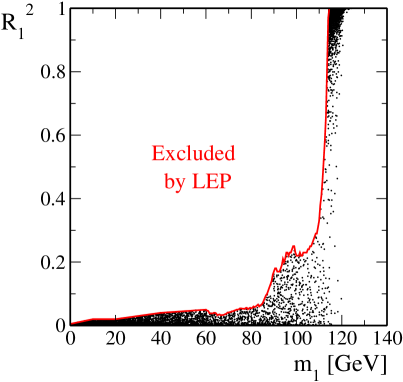
In Fig. 2 we plot the square of the reduced coupling of the lightest Higgs state, $R_{1}^{2}$, versus $m_{1}$ for the same set of points as in Fig. 1. We also display the LEP exclusion curve [14], from which one can see that the light $h_{1}$ states are indeed not excluded. The presence of a light Higgs state with a small reduced coupling to the SM gauge bosons might prove difficult to detect at future colliders. However, it is worth stressing that in our results we always have at least one light visible Higgs state with a large reduced coupling to the gauge bosons ($R_{i}^{2}\raise 1.29167pt\hbox{$>$\kern-7.5pt\raise-4.73611pt\hbox{$\sim$}}0.5$) and a mass in the interval $112~{}{\rm GeV}\raise 1.29167pt\hbox{$<$\kern-7.5pt\raise-4.73611pt\hbox{$\sim$}}m_{i}\raise 1.29167pt\hbox{$<$\kern-7.5pt\raise-4.73611pt\hbox{$\sim$}}150~{}{\rm GeV}$. The lower bound is fixed by the LEP limit as shown in Fig. 2. The upper bound can be understood from the following relation

$$\sum_{i=1}^{5}R_{i}^{2}m_{i}^{2}=\cos^{2}\beta M_{11}^{2}+2\cos\beta\sin\beta M_{12}^{2}+\sin^{2}\beta M_{22}^{2}\;,$$ (3.5)

where $M_{11}^{2},M_{12}^{2},M_{22}^{2}$ are the Higgs boson mass matrix elements as given in the previous section. The right hand side of Eq. (3.5) gives the usual NMSSM upper bound on the lightest Higgs boson mass [33], with the only difference being that the stop mixing parameter $X_{t}$ now depends on the CP violating phase $\theta$, as seen in Eq. (2.13).

Assuming $m_{t}^{\mathrm{p}ole}=175~{}{\rm GeV}$, $M_{\mathrm{S}USY}=350~{}{\rm GeV}$ and maximal stop mixing, one obtains $m_{1}\raise 1.29167pt\hbox{$<$\kern-7.5pt\raise-4.73611pt\hbox{$\sim$}}125~{}{\rm GeV}$ with this upper bound being saturated for small $\tan\beta$, namely $\tan\beta\simeq 2.7$ [33]. One can check from Figs. 1 and 2 that this upper bound is only reached by a few points in our set. The dense band of points in Fig. 1 corresponds to cases where $h_{1}$ is a SM-like Higgs state with $R_{1}\simeq 1$. In this case, the lower bound from LEP is $m_{1}\raise 1.29167pt\hbox{$>$\kern-7.5pt\raise-4.73611pt\hbox{$\sim$}}114~{}{\rm GeV}$ and the upper bound, from Eq. (3.5), is $m_{1}\raise 1.29167pt\hbox{$<$\kern-7.5pt\raise-4.73611pt\hbox{$\sim$}}125~{}{\rm GeV}$ as explained above.

We have also applied the exclusion limit from LEP on Higgs bosons associated production ($e^{+}e^{-}\rightarrow hA$ in the MSSM). This provides an upper bound on the $Zh_{i}h_{j}$ reduced coupling as a function of $m_{i}+m_{j}$ for $m_{i}\simeq m_{j}$ [15]. The $Zh_{i}h_{j}$ reduced coupling is the equivalent of $\cos(\beta-\alpha)$ in the MSSM and is here defined as

$$R^{\prime}_{ij}=h_{i4}(h_{j2}\cos\beta-h_{j1}\sin\beta)-(i\leftrightarrow j)\;,$$ (3.6)

with $h_{i4}$ the CP-odd doublet $P$ component of $h_{i}$. We have also taken into account the LEP limit on the charged Higgs boson mass [16], which here simply reads $m_{H^{\pm}}>89.6~{}{\rm GeV}$. By inspection of Eq. (2.24), this limit translates into having opposite signs for the phases $\theta$ and $\delta$.

As we will see in the next section, charginos play an important role in the computation of $\varepsilon_{K}$. The tree level chargino mass matrix in the $(\tilde{W},\tilde{H})$ basis reads

$${\cal M}_{\tilde{\chi}^{\pm}}=\left(\begin{array}[]{cc}M_{2}&\sqrt{2}M_{W}\sin\beta e^{-i\theta}\\ \sqrt{2}M_{W}\cos\beta&-\lambda x\end{array}\right)\;,$$ (3.7)

where $M_{2}$ is the soft wino mass. We randomly scanned in the following interval for $M_{2}$

$$100~{}{\rm GeV}<M_{2}<250~{}{\rm GeV}$$ (3.8)

and applied the LEP bound on the chargino mass, $m_{\tilde{\chi}^{\pm}_{1,2}}>103.5~{}{\rm GeV}$ [34]. Finally, we checked that for each point the stop masses also satisfied the associated LEP limit $m_{\tilde{t}_{1,2}}>100~{}{\rm GeV}$ [35].

4 Indirect CP violation in $K^{0}-\bar{K}^{0}$ mixing

In the framework of the NMSSM with SCPV, all the SUSY parameters are real. Even so, the physical phases of the Higgs doublets and singlet appear in the scalar fermion, chargino and neutralino mass matrices, as well as in several interaction vertices. In this section we will explore whether or not these physical phases can account for the experimental value of $\varepsilon_{K}$, $\varepsilon_{K}=(2.271\pm 0.017)\times 10^{-3}$ [36].

It is worth stressing that in this scenario the SM does not provide any contribution to the CP violating observables, since the CKM matrix is real. This can be clarified by noting that since $N$ is a singlet field, it does not couple to the quarks, and although both Higgs doublets do couple, the phase associated with these couplings can be rotated away by means of a redefinition of the right-handed quark fields. Since charged currents are purely left-handed, these phases do not show up in the $V_{\mathrm{CKM}}$, which is thus real.

Let us now proceed to compute the contributions to the indirect CP violation parameter of the kaon sector, which is defined as

$$\varepsilon_{K}\simeq\frac{e^{i\pi/4}}{\sqrt{2}}\frac{\operatorname{Im}\mathcal{M}_{12}}{\Delta m_{K}}\;.$$ (4.1)

In the latter $\Delta m_{K}$ is the long- and short-lived kaon mass difference, and $\mathcal{M}_{12}$ is the off-diagonal element of the neutral kaon mass matrix, which is related to the effective hamiltonian that governs $\Delta S=2$ transitions as

$$\mathcal{M}_{12}=\frac{\langle K^{0}|\mathcal{H}_{\text{eff}}^{\Delta S=2}|\bar{K}^{0}\rangle}{2m_{K}}\;,\quad\text{with}\qquad\mathcal{H}_{\text{eff}}^{\Delta S=2}=\sum_{i}c_{i}{\mathcal{O}}_{i}\;.$$ (4.2)

Here $c_{i}$ are the Wilson coefficients and ${\mathcal{O}}_{i}$ the local operators. In the presence of SUSY contributions, the Wilson coefficients can be decomposed as $c_{i}=c_{i}^{W}+c_{i}^{H^{\pm}}+c_{i}^{\tilde{\chi}^{\pm}}+c_{i}^{\tilde{g}}+c_{i}^{\tilde{\chi}^{0}}$. As discussed in [23], in the present class of models where there are no contributions from the SM, the chargino mediated box diagrams give the leading supersymmetric contribution, and the $\Delta S=2$ transition is largely dominated by the $(V-A)$ four fermion operator $\mathcal{O}_{1}$. Working in the weak basis for the $\tilde{W}-\tilde{H}$, rather than in the physical chargino basis, and using the mass insertion approximation for the internal squarks, we have verified that the $\varepsilon_{K}$ receives the leading contribution from the box diagrams depicted in Fig. 3. In the limit of degenerate masses for the left-handed up-squarks, $\operatorname{Im}\mathcal{M}_{12}$ is given by [23]

Figure 3: Box diagrams associated with the leading chargino contribution to $\varepsilon_{K}$.

$$\operatorname{Im}\mathcal{M}_{12} = \frac{2G_{F}^{2}f^{2}_{K}m_{K}m_{W}^{4}}{3\pi^{2}\langle m_{\tilde{q}}\rangle^{8}}(V_{td}^{*}V_{ts})m_{t}^{2}\left|e^{i\theta}\;m_{\tilde{W}}-\cot\beta\;m_{\tilde{H}}\right|$$ (4.3)

$$\times\left\{\Delta A_{U}\sin[\varphi_{\chi}-\theta]\;{(M^{2}_{\tilde{Q}})}_{12}\;I(r_{\tilde{W}},r_{\tilde{H}},r_{\tilde{u}_{L}},r_{\tilde{t}_{R}})\right\}\;.$$

In the above equation, $f_{K}$ is the kaon decay constant and $m_{K}$ the kaon mass [36]; $V_{ij}$ are the $V_{\mathrm{CKM}}$ elements, whose numerical values ($V_{td}=0.0066$ and $V_{ts}=-0.04$) reflect the fact that we are dealing with a flat unitarity triangle; $\langle m_{\tilde{q}}\rangle$ is the average squark mass, which we take equal to $M_{\rm SUSY}$; $m_{\tilde{W}}=M_{2}$ is the wino mass, $m_{\tilde{H}}=\mu$ is the higgsino mass and $\varphi_{\chi}=\arg(e^{i\theta}m_{{\tilde{W}}}-\cot\beta\;m_{{\tilde{H}}})$. The non-universality in the $LL$ soft breaking masses is parametrized by ${(M^{2}_{\tilde{Q}})}_{12}$, which we choose taking into account the bounds from the analysis in Ref. [37]. As discussed in Ref. [23], a sizable non-universality in the soft trilinear terms is crucial, and is here parametrized by $\Delta A_{U}\equiv A_{U}^{13}-A_{U}^{23}$. In the following, we assume $\Delta A_{U}=500~{}{\rm GeV}$. Finally, $I$ is the loop function, with $r_{i}=m_{i}^{2}/\langle m_{\tilde{q}}\rangle^{2}$ [23].

By scanning the parameter space of the model, we have verified that one can find sets of parameters that satisfy the minimization conditions of the Higgs potential, have an associated Higgs boson spectrum compatible with LEP searches and still succeed in generating the observed value of $\varepsilon_{K}$. From Eq. (4.3), it appears that $\varepsilon_{K}$ depends on $1/M_{\rm SUSY}^{8}$. It is therefore difficult to saturate the experimental value of $\varepsilon_{K}$ for large values of $M_{\rm SUSY}$. On the other hand, too small values of $M_{\rm SUSY}$ might generate a light Higgs boson spectrum, already excluded by LEP. In order to accommodate both constraints, we took $M_{\rm SUSY}=350~{}{\rm GeV}$, as already referred to in section 3. All other parameters are as in Eqs. (3, 3.8) and we assumed $m_{t}^{\rm pole}=175~{}{\rm GeV}$ and maximal stop mixing, as in the previous section.

Figure 4: Values of $\varepsilon_{K}$ as function of $\tan\beta$ (shaded area) for $m_{t}^{\rm pole}=175~{}{\rm GeV}$, $M_{\rm SUSY}=350~{}{\rm GeV}$ and maximal stop mixing. The other parameters are randomly chosen as in Eqs. (3, 3.8).

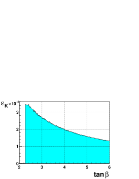
In Fig. 4, we plot the possible values of $\varepsilon_{K}$ as a function of $\tan\beta$. The maximal values of $\varepsilon_{K}$ are obtained for the low $\tan\beta$ regime, and the experimental bounds on $\varepsilon_{K}$ require $\tan\beta\raise 1.29167pt\hbox{$<$\kern-7.5pt\raise-4.73611pt\hbox{$\sim$}}3.8$. Recall that the lower bound for $\tan\beta$ is consistent with the analysis conducted in section 3. Apart from the explicit dependence of Eq. (4.3) on $\tan\beta$, one should bear in mind that there are also implicit dependences associated with the other parameters as well as with the various experimental bounds imposed on the mass spectrum. It is therefore difficult to reproduce analytically the observed upper bound on $\varepsilon_{K}$ as a function of $\tan\beta$.

Figure 5: Contours for the maximum value of $\varepsilon_{K}$ in the $\lambda$–$\kappa$ plane for $m_{t}^{\rm pole}=175~{}{\rm GeV}$, $M_{\rm SUSY}=350~{}{\rm GeV}$, maximal stop mixing and the other parameters as in Eqs. (3, 3.8).

Figure 6: Contours for the maximum value of $\varepsilon_{K}$ in the $\theta$–$\delta$ plane. All parameters as in Fig. 5.

Figure 7: Values of $\varepsilon_{K}$ as function of the singlet phase $\varphi_{3}=\delta/3$ (grey area). All parameters as in Fig. 5.

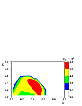
In Fig. 5, we plot the maximal value of $\varepsilon_{K}$ in distinct regions of the $\lambda-\kappa$ plane. The remaining parameters are chosen in order to maximize $\varepsilon_{K}$ and still comply with the experimental bounds. As one can see from this figure, having $\varepsilon_{K}\sim 2\times 10^{-3}$ is associated with values of $\kappa$ and $\lambda$ in the range $[0,0.6]$. In other words, one can easily saturate $\varepsilon_{K}$ in a vast region of the parameter space.

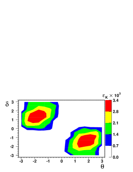
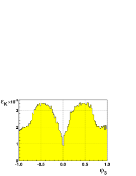
As expected from the inspection of Eq. (4.3), there is a strong dependence of $\varepsilon_{K}$ on the phases associated with the Higgs fields. In Fig. 6, we display contour plots for the maximal values of $\varepsilon_{K}$ in the plane generated by the phases $\theta$ and $\delta$. Although, a priori, all the values for the phases $\theta$ and $\delta$ in $[-\pi,\pi]$ are allowed, it is clear from Fig. 6 that the saturation of the experimental value of $\varepsilon_{K}$ can only be achieved for significant values of the singlet and doublet phases. This feature becomes more evident in Fig. 7, where we show the values of $\varepsilon_{K}$ as a function of the singlet phase, $\varphi_{3}=\delta/3$. The saturation of the experimental value of $\varepsilon_{K}$ requires the singlet phase to be $|\varphi_{3}|\gtrsim 0.15$. We will discuss in the conclusions the implications of such large CP violating phases.

5 Conclusions and discussion

We have shown that in the framework of the NMSSM with an extra tadpole term for the singlet in the scalar potential, it is possible to have spontaneous CP violation while complying with the LEP constraints on the Higgs boson mass. Although in this scenario $V_{\mathrm{CKM}}$ is real, the experimental value of $\varepsilon_{K}$ can be saturated in large parts of the parameter space of the model, without requiring any fine tuning. This may be of special interest for electroweak baryogenesis, as it has been shown that a strong first order electroweak phase transition is possible in the NMSSM, as opposed to the MSSM, due to the additional trilinear Higgs boson couplings in the lagrangian [39].

The presence of the extra tadpole term $\xi$ is crucial to conciliate spontaneous CP violation with the LEP constraints on the Higgs boson mass. Moreover, the $\xi$ term also solves the domain wall problem associated with the spontaneous breaking of the $\mathbb{Z}_{3}$ symmetry, which is present if $\xi=0$. On the other hand, since CP is spontaneously broken at the electroweak scale, CP domain walls may appear, which are cosmologically excluded. An elegant solution to this problem, along the lines of the $\mathbb{Z}_{3}$ domain walls solution, is to assume that gravitational interactions also explicitly break CP. In the low energy scalar potential, one then obtains an explicit CP violating tadpole term, i.e. a complex $\xi$ term. A phase in the $\xi$ term would not change the results derived here, since its only effect is to generate a shift in the singlet phase $\delta$.

Regarding the large phase regime favoured by the saturation of $\varepsilon_{K}$, one should recall that $\theta$ and $\delta$ are flavour-conserving phases, and might generate sizable contributions to the electron, neutron and mercury atom EDMs. Although we will not address the EDM problem here, a few remarks are in order: first, let us notice that in the presence of a small singlet coupling $\lambda$, as allowed in our results (see Fig. 5), the EDM constraints on $\delta$ become less stringent [38]. In addition, there are several possible ways to evade the EDM problem, namely reinforcing the non-universality on the trilinear terms (i.e. requiring the diagonal terms to be much smaller than the off-diagonal ones or having matrix-factorizable $A$ terms), the existence of cancellations between the several SUSY contributions, and the suppression of the EDMs by a heavy SUSY spectrum [6]. In view of the considerably large parameter space allowed in our results, none of these possibilities should be disregarded.

Concerning the other CP-violating observables, namely $\varepsilon^{\prime}/\varepsilon$ and the CP asymmetry of the $B_{d}$ meson decay ($a_{J/\psi K_{S}}$), it has been pointed out that this class of models can generate sizable contributions, although saturating the experimental values generally favours a regime of large phases and maximal $LR$ squark mixing [21, 40]. A complete analysis of these issues, as well as of the EDM problem in our model has yet to be done.

In this work, we pointed out that the NMSSM with an extra tadpole term in the scalar potential appears to be an excellent candidate for a scenario of SCPV. Having a $\mathbb{Z}_{3}$ invariant superpotential preserves the original motivation of the NMSSM to solve the $\mu$ problem of supersymmetry. The extra tadpole term for the singlet cures the domain wall problem of the $\mathbb{Z}_{3}$ invariant model and allows the spontaneous breaking of CP. In this model, one can simultaneously saturate $\varepsilon_{K}$ and obtain a particle spectrum compatible with the current experimental bounds.

The presently available experimental data on CP violation does not allow to distinguish whether the CP symmetry is spontaneously or explicitly broken. With the advent of the LHC and eventually of the Linear Collider, direct searches of the Higgs bosons, and the measurement the associated couplings to the SM gauge bosons, will allow to disentangle this model from the MSSM.

Acknowledgments

This work was supported by the Spanish grant BFM2002-00345 and by the European Commission RTN grant HPRN-CT-2000-00148. A. T. was supported by Fundação para a Ciência e Tecnologia under the grant SFRH/BPD/11509/2002. J.C.R. was partly supported by the Marie Curie fellowship HPMF-CT-2002-01902.

References

• [1] J.H. Christenson, J.W. Cronin, V.L. Fitch, R. Turlay, Phys. Rev. Lett. 13 (1964) 138.
• [2] N. Cabibbo, Phys. Rev. Lett. 10 (1963) 531;
M. Kobayashi, K. Maskawa, Prog. Theor. Phys. 49 (1973) 652.
• [3] M.B. Gavela, P. Hernandez, J. Orloff, O. Pene, C. Quimbay, Nucl. Phys. B 430 (1994) 382.
• [4] G. ’t Hooft et al (Eds.), Recent Developments in Gauge Theories, Proceedings of the Nato Advanced Summer Institute (Cargèse, 1979), Plenum, New York, 1980.
• [5] S. Khalil, T. Kobayashi, A. Masiero, Phys. Rev. D 60 (1999) 075003;
S. Khalil, T. Kobayashi, Phys. Lett. B 460 (1999) 341;
G. C. Branco et al, arXiv:hep-ph/0204136, to appear in Nucl. Phys. B.
• [6] S. Khalil, arXiv:hep-ph/0212050.
• [7] T.D. Lee, Phys. Rev. D 8 (1973) 1226;
S. Weinberg, Phys. Rev. Lett. 37 (1976) 657.
• [8] R.N. Mohapatra, G. Senjanovic, Phys. Lett. B 79 (1978) 283;
S.M. Barr, P. Langacker, Phys. Rev. Lett. 42 (1979) 1654;
H. Georgi, Hadronic Journal 1 (1981) 155;
A.E. Nelson, Phys. Lett. B 136 (1984) 387, Phys. Lett. B 143 (1984) 165;
S.M. Barr, Phys. Rev. Lett. 53 (1984) 329.
• [9] A. Strominger, E. Witten, Commun. Math. Phys. 101 (1985) 341.
• [10] for a review, see J.F. Gunion, G.L. Kane, H.E. Haber, S. Dawson, The Higgs Hunter’s Guide Addison Wesley (1990).
• [11] N. Maekawa, Phys. Lett. B 282 (1992) 387.
• [12] H. Georgi, A. Pais, Phys. Rev. D 10 (1974) 1246.
• [13] A. Pomarol, Phys. Lett. B 287 (1992) 331.
• [14] LEP Higgs Working Group, Note 2002/01.
• [15] LEP Higgs Working Group, Note 2001/04.
• [16] LEP Higgs working group, Note 2001/05.
• [17] H.-P. Nilles, M. Srednicki, D. Wyler, Phys. Lett. B 120 (1983) 346.
• [18] J. Ellis, J.F. Gunion, H.E. Haber, L. Roszkowski, F. Zwirner, Phys. Rev. D 39 (1989) 844.
• [19] J. C. Romão, Phys. Lett. B 173 (1986) 309.
• [20] K.S. Babu, S.M. Barr, Phys. Rev. D 49 (1994) 2156.
• [21] A. Pomarol, Phys. Rev. D 47 (1993) 273.
• [22] A.T. Davies, C.D. Frogatt, A. Usai, Phys. Lett. B 517 (2001) 375.
• [23] G. C. Branco, F. Krüger, J. C. Romão, A. M. Teixeira, JHEP 0107 (2001) 027.
• [24] U. Ellwanger, Phys. Lett. B 133 (1983) 187.
• [25] S.A. Abel, Nucl. Phys. B 480 (1996) 55.
• [26] S.A. Abel, S. Sarkar, P.L. White, Nucl. Phys. B 454 (1995) 663.
• [27] K. Tamvakis, C. Panagiotakopoulos, Phys. Lett. B 446 (1999) 224.
• [28] K. Tamvakis, C. Panagiotakopoulos, Phys. Lett. B 469 (1999) 145;
A. Dedes, C. Hugonie, S. Moretti, K. Tamvakis, Phys. Rev. D 63 (2001) 055009;
C. Panagiotakopoulos, A. Pilaftsis, Phys. Rev. D 63 (2001) 055003, Phys. Lett. B 505 (2001) 184.
• [29] N. Haba, M. Matsuda, M. Tanimoto, Phys. Rev. D 54 (1996) 6928;
S.W. Ham, S.K. Oh, H.S. Song, Phys. Rev. D 61 (2000) 055010.
• [30] Y. Okada, M. Yamaguchi, T. Yanagida, Prog. Theor. Phys. 85 (1991) 1, Phys. Lett. B 262 (1991) 54;
A. Yamada, Phys. Lett. B 263 (1991) 233;
J. Ellis, G. Ridolfi, F. Zwirner, Phys. Lett. B 257 (1991) 83, Phys. Lett. B 262 (1991) 477;
A. Brignole, J. Ellis, G. Ridolfi, F. Zwirner, Phys. Lett. B 271 (1991) 167;
R. Barbieri, M. Frigeni, F. Caravaglios, Phys. Lett. B 258 (1991) 167;
H. Haber, R. Hempfling, Phys. Rev. Lett. 66 (1991) 1815.
• [31] U. Ellwanger, Phys. Lett. B 303 (1993) 271;
T. Elliott, S.F. King, P.L. White, Phys. Lett. B 305 (1993) 71, Phys. Lett. B 314 (1993) 56, Phys. Rev. D 49 (1994) 2435.
• [32] M. Carena, H.E. Haber, S. Heinemeyer, W. Hollik, C.E.M. Wagner, G. Weiglein, Nucl. Phys. B 580 (2000) 29;
J. R. Espinosa, R.-J. Zhang, Nucl. Phys. B 586 (2000) 3;
A. Brignole, G. Degrassi, P. Slavich, F. Zwirner, Nucl. Phys. B 631 (2002) 195.
• [33] U. Ellwanger, C. Hugonie, Eur. Phys. J. C 25 (2002) 297.
• [34] LEP SUSY Working Group, Note 01-03.1.
• [35] LEP SUSY Working Group, Note 02-02.1.
• [36] K. Hagiwara et al. [Particle Data Group Collaboration], Phys. Rev. D 66 (2002) 010001.
• [37] M. Ciuchini et al., JHEP 10 (1998) 008.
• [38] M. Matsuda, M. Tanimoto, Phys. Rev. D 52 (1995) 3100.
• [39] M. Pietroni, Nucl. Phys. B 402 (1993) 27;
A.T. Davies, C.D. Froggatt, R.G. Moorhouse, Phys. Lett. B 372 (1996) 88;
S.J. Huber, M.G. Schmidt, Eur. Phys. J. C 10 (1999) 473;
M. Bastero-Gil, C. Hugonie, S. F. King, D. P. Roy, S. Vempati, Phys. Lett. B 489 (2000) 359.
• [40] O. Lebedev, Int. J. Mod. Phys. A15 (2000) 2987.