CERN-TH/2003-084

hep-ph/0304027

New Strategies to Obtain Insights into CP Violation Through
$B_{s}\to D_{s}^{\pm}K^{\mp},D_{s}^{\ast\pm}K^{\mp},...$ and $B_{d}\to D^{\pm}\pi^{\mp},D^{\ast\pm}\pi^{\mp},...$ Decays

Robert Fleischer

Theory Division, CERN, CH-1211 Geneva 23, Switzerland

Decays of the kind $B_{s}\to D_{s}^{\pm}K^{\mp},D_{s}^{\ast\pm}K^{\mp},...$ and $B_{d}\to D^{\pm}\pi^{\mp},D^{\ast\pm}\pi^{\mp},...$ allow us to probe $\phi_{s}+\gamma$ and $\phi_{d}+\gamma$, respectively, involving the angle $\gamma$ of the unitarity triangle and the $B^{0}_{q}$–$\overline{B^{0}_{q}}$ mixing phases $\phi_{q}$ ($q\in\{d,s\}$). Analysing these modes in a phase-convention-independent way, we find that their mixing-induced observables are affected by a subtle $(-1)^{L}$ factor, where $L$ denotes the angular momentum of the $B_{q}$ decay products, and derive bounds on $\phi_{q}+\gamma$. Moreover, we emphasize that “untagged” rates are an important ingredient for efficient determinations of weak phases, not only in the presence of a sizeable width difference $\Delta\Gamma_{q}$; should $\Delta\Gamma_{s}$ be sizeable, the combination of “untagged” with “tagged” $B_{s}\to D_{s}^{\pm}K^{\mp},D_{s}^{\ast\pm}K^{\mp},...$ observables provides an elegant and unambiguous extraction of $\tan(\phi_{s}+\gamma)$, whereas the “conventional” determination of $\phi_{s}+\gamma$ is affected by an eightfold discrete ambiguity. Finally, we propose a combined analysis of $B_{s}\to D_{s}^{\pm}K^{\mp},D_{s}^{\ast\pm}K^{\mp},...$ and $B_{d}\to D^{\pm}\pi^{\mp},D^{\ast\pm}\pi^{\mp},...$ modes, which has important advantages, offering various interesting new strategies to extract $\gamma$ in an essentially unambiguous manner.

CERN-TH/2003-084
April 2003

1 Introduction

The exploration of CP violation through studies of $B$-meson decays is one of the most exciting topics of present particle physics phenomenology, the main goal being to perform stringent tests of the Kobayashi–Maskawa mechanism [1]. Here the central target is the unitarity triangle of the Cabibbo–Kobayashi–Maskawa (CKM) matrix, with its angles $\alpha$, $\beta$ and $\gamma$ (for a detailed review, see [2]). Thanks to the efforts of the BaBar (SLAC) and Belle (KEK) collaborations, CP violation could recently be established in the neutral $B_{d}$-meson system with the help of $B_{d}\to J/\psi K_{\rm S}$ and similar decays [3]. These modes allow us to determine $\sin\phi_{d}$, where the present world average is given by $\sin\phi_{d}=0.734\pm 0.054$ [4], implying the twofold solution $\phi_{d}=(47^{+5}_{-4})^{\circ}\lor(133^{+4}_{-5})^{\circ}$ for the $B^{0}_{d}$–$\overline{B^{0}_{d}}$ mixing phase $\phi_{d}$, which equals $2\beta$ in the Standard Model. Here the former solution would be in perfect agreement with the “indirect” range following from the Standard-Model “CKM fits”, $40^{\circ}\mathrel{\hbox to0.0pt{\lower 3.0pt\hbox{$\mathchar 536\relax$}\hss}\raise 2.0pt\hbox{$\mathchar 316\relax$}}\phi_{d}\mathrel{\hbox to0.0pt{\lower 3.0pt\hbox{$\mathchar 536\relax$}\hss}\raise 2.0pt\hbox{$\mathchar 316\relax$}}60^{\circ}$ [5], whereas the latter would correspond to new physics [6]. Measuring the sign of $\cos\phi_{d}$, the two solutions can be distinguished. Several strategies to accomplish this important task were proposed [7]; an analysis using the time-dependent angular distribution of the decay products of $B_{d}\to J/\psi[\to\ell^{+}\ell^{-}]K^{\ast}[\to\pi^{0}K_{\rm S}]$ [8, 9] is already in progress at the $B$ factories [10].

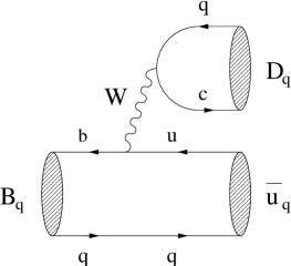
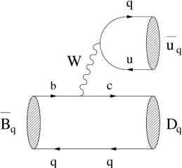
Figure 1: Feynman diagrams contributing to $B_{q}^{0}\to D_{q}\overline{u}_{q}$ and $\overline{B_{q}^{0}}\to D_{q}\overline{u}_{q}$.

An important ingredient for the testing of the Kobayashi–Maskawa picture is provided by transitions of the kind $B_{s}\to D_{s}^{\pm}K^{\mp},D_{s}^{\ast\pm}K^{\mp},...$ [11] and $B_{d}\to D^{\pm}\pi^{\mp},D^{\ast\pm}\pi^{\mp},...$ [12], allowing theoretically clean determinations of the weak phases $\phi_{s}+\gamma$ and $\phi_{d}+\gamma$, respectively, where $\phi_{s}$ is the $B_{s}$-meson counterpart of $\phi_{d}$, which is negligibly small in the Standard Model. It is convenient to write these decays generically as $B^{0}_{q}\to D_{q}\overline{u}_{q}$, so that we may easily distinguish between the following cases:

• $q=s$: $D_{s}\in\{D_{s}^{+},D_{s}^{\ast+},...\}$, $u_{s}\in\{K^{+},K^{\ast+},...\}$,

• $q=d$: $D_{d}\in\{D^{+},D^{\ast+},...\}$, $u_{d}\in\{\pi^{+},\rho^{+},...\}$.

In the discussion given below, we shall only consider $B^{0}_{q}\to D_{q}\overline{u}_{q}$ decays, where at least one of the $D_{q}$, $\overline{u}_{q}$ states is a pseudoscalar meson. In the opposite case, for example the $B^{0}_{s}\to D_{s}^{\ast+}K^{\ast-}$ decay, the extraction of weak phases would require a complicated angular analysis [13]–[15]. If we look at Fig. 1, we observe that $B^{0}_{q}\to D_{q}\overline{u}_{q}$ originates from colour-allowed tree-diagram-like topologies, and that also a $\overline{B^{0}_{q}}$ meson may decay into the same final state $D_{q}\overline{u}_{q}$. The latter feature leads to interference effects between $B^{0}_{q}$–$\overline{B^{0}_{q}}$ mixing and decay processes, allowing the extraction of $\phi_{q}+\gamma$ with an eightfold discrete ambiguity. Since $\phi_{q}$ can be straightforwardly fixed separately [2], we may determine the angle $\gamma$ of the unitarity triangle from this CP-violating weak phase.

In Section 2, we focus on the $B_{q}\to D_{q}\overline{u}_{q}$ decay amplitudes and rate asymmetries, and investigate the relevant hadronic parameters with the help of “factorization”. In this section, we shall also point out that a subtle factor $(-1)^{L}$ arises in the expressions for the mixing-induced observables, where $L$ denotes the angular momentum of the $D_{q}\overline{u}_{q}$ system, and show explicitly the cancellation of phase-convention-dependent parameters within the factorization approach. After discussing the “conventional” extraction of $\phi_{q}+\gamma$ and the associated multiple discrete ambiguities in Section 3, we emphasize the usefulness of “untagged” rate measurements for efficient determinations of weak phases from $B_{q}\to D_{q}\overline{u}_{q}$ decays in Section 4, and suggest several novel strategies. In Section 5, we then derive bounds on $\phi_{q}+\gamma$, and illustrate their potential power with the help of a few numerical examples. In Section 6, we propose a combined analysis of $B_{s}\to D_{s}\overline{u}_{s}$ and $B_{d}\to D_{d}\overline{u}_{d}$ modes, which has important advantages with respect to the conventional separate determinations of $\phi_{s}+\gamma$ and $\phi_{d}+\gamma$, offering various attractive new avenues to extract $\gamma$ in an essentially unambiguous manner and to obtain valuable insights into hadron dynamics. Finally, we conclude in Section 7.

2 Amplitudes, Rate Asymmetries and Factorization

2.1 Amplitudes

The $B_{q}\to D_{q}\overline{u}_{q}$ decays are the colour-allowed counterparts of the $B_{s}\to D\eta^{(^{\prime})},D\phi,...$ and $B_{d}\to D\pi^{0},D\rho^{0},...$ channels, which were recently analysed in detail in [16, 17]. If we follow the same avenue, and take also the Feynman diagrams shown in Fig. 1 into account, we may write

$$A(\overline{B^{0}_{q}}\to D_{q}\overline{u}_{q})=\langle\overline{u}_{q}D_{q}|{\cal H}_{\rm eff}(\overline{B^{0}_{q}}\to D_{q}\overline{u}_{q})|\overline{B^{0}_{q}}\rangle=\frac{G_{\rm F}}{\sqrt{2}}\overline{v}_{q}\overline{M}_{q},$$ (2.1)

where the hadronic matrix element

$$\overline{M}_{q}\equiv\langle\overline{u}_{q}D_{q}|\overline{{\cal O}}_{1}^{\,q}\,{C}_{1}(\mu)+\overline{{\cal O}}_{2}^{\,q}\,{C}_{2}(\mu)|\overline{B^{0}_{q}}\rangle$$ (2.2)

involves the current–current operators

$$\overline{{\cal O}}_{1}^{\,q}\equiv(\overline{q}_{\alpha}u_{\beta})_{\mbox{{\scriptsize V--A}}}\left(\overline{c}_{\beta}b_{\alpha}\right)_{\mbox{{\scriptsize V--A}}},\quad\overline{{\cal O}}_{2}^{\,q}\equiv(\overline{q}_{\alpha}u_{\alpha})_{\mbox{{\scriptsize V--A}}}\left(\overline{c}_{\beta}b_{\beta}\right)_{\mbox{{\scriptsize V--A}}}.$$ (2.3)

The CKM factors $\overline{v}_{q}$ are given by

$$\overline{v}_{s}\equiv V_{us}^{\ast}V_{cb}=A\lambda^{3},\quad\overline{v}_{d}\equiv V_{ud}^{\ast}V_{cb}=A\lambda^{2}(1-\lambda^{2}/2),$$ (2.4)

with (for the numerical value, see [18])

$$A\equiv\frac{1}{\lambda^{2}}|V_{cb}|=0.83\pm 0.02,$$ (2.5)

and $\lambda\equiv|V_{us}|=0.22$ is the usual Wolfenstein parameter [19].

On the other hand, the $B^{0}_{q}\to D_{q}\overline{u}_{q}$ decay amplitude takes the following form:

$$A(B^{0}_{q}\to D_{q}\overline{u}_{q})=\langle\overline{u}_{q}D_{q}|{\cal H}_{\rm eff}(B^{0}_{q}\to D_{q}\overline{u}_{q})|B^{0}_{q}\rangle$$ (2.6)

$$=\frac{G_{\rm F}}{\sqrt{2}}v_{q}^{\ast}\langle\overline{u}_{q}D_{q}|{\cal O}_{1}^{q\dagger}\,{C}_{1}(\mu)+{\cal O}_{2}^{q\dagger}\,{C}_{2}(\mu)|B^{0}_{q}\rangle,$$

where we have to deal with the current–current operators

$${\cal O}_{1}^{q}\equiv(\overline{q}_{\alpha}c_{\beta})_{\mbox{{\scriptsize V--A}}}\left(\overline{u}_{\beta}b_{\alpha}\right)_{\mbox{{\scriptsize V--A}}},\quad{\cal O}_{2}^{q}\equiv(\overline{q}_{\alpha}c_{\alpha})_{\mbox{{\scriptsize V--A}}}\left(\overline{u}_{\beta}b_{\beta}\right)_{\mbox{{\scriptsize V--A}}},$$ (2.7)

and the CKM factors $v_{q}$ are given by

$$v_{s}\equiv V_{cs}^{\ast}V_{ub}=A\lambda^{3}R_{b}e^{-i\gamma},\quad v_{d}\equiv V_{cd}^{\ast}V_{ub}=-\left(\frac{A\lambda^{4}R_{b}}{1-\lambda^{2}/2}\right)e^{-i\gamma},$$ (2.8)

with (for the numerical value, see [18])

$$R_{b}\equiv\left(1-\frac{\lambda^{2}}{2}\right)\frac{1}{\lambda}\left|\frac{V_{ub}}{V_{cb}}\right|=\sqrt{\overline{\rho}^{2}+\overline{\eta}^{2}}=0.39\pm 0.04.$$ (2.9)

If we introduce convention-dependent CP phases through

$$({\cal CP})|F\rangle=e^{i\phi_{\rm CP}(F)}|\overline{F}\rangle,\quad({\cal CP})|\overline{F}\rangle=e^{-i\phi_{\rm CP}(F)}|F\rangle$$ (2.10)

for $F\in\{B_{q},D_{q},u_{q}\}$, we obtain

$$({\cal CP})|D_{q}\overline{u}_{q}\rangle=(-1)^{L}e^{i[\phi_{\rm CP}(D_{q})-\phi_{\rm CP}(u_{q})]}|\overline{D}_{q}u_{q}\rangle,$$ (2.11)

where $L$ denotes the angular momentum of the $D_{q}\overline{u}_{q}$ state. As we shall see below, the subtle $(-1)^{L}$ factor enters in mixing-induced observables, and plays an important rôle for the extraction of weak phases from these quantities in the presence of non-trivial angular momenta, for instance in the case of $B^{0}_{d}\to D^{\ast+}\pi^{-}$. In the literature, this factor does not show up explicitly in the context of $B^{0}_{q}\to D_{q}\overline{u}_{q}$ modes, but it was recently pointed out in the analysis of their colour-suppressed counterparts in [16, 17]. If we now employ, as in these papers, the operator relations

$$({\cal CP})^{\dagger}({\cal CP})=\hat{1},$$ (2.12)

$$({\cal CP}){\cal O}_{k}^{q\dagger}({\cal CP})^{\dagger}={\cal O}_{k}^{q},$$ (2.13)

we may rewrite (2.6) as

$$A(B^{0}_{q}\to D_{q}\overline{u}_{q})=(-1)^{L}e^{i[\phi_{\rm CP}(B_{q})-\phi_{\rm CP}(D_{q})+\phi_{\rm CP}(u_{q})]}\frac{G_{\rm F}}{\sqrt{2}}v_{q}^{\ast}M_{q},$$ (2.14)

where

$$M_{q}\equiv\langle u_{q}\overline{D}_{q}|{\cal O}_{1}^{q}\,{C}_{1}(\mu)+{\cal O}_{2}^{q}\,{C}_{2}(\mu)|\overline{B^{0}_{q}}\rangle.$$ (2.15)

It should be noted that also certain exchange topologies contribute to $B^{0}_{q}\to D_{q}\overline{u}_{q}$, $\overline{B^{0}_{q}}\to D_{q}\overline{u}_{q}$ transitions, which were – for simplicity – not shown in Fig. 1. However, these additional diagrams do not affect the phase structure of the amplitudes in (2.1) and (2.14), and manifest themselves only through tiny contributions to the hadronic matrix elements $\overline{M}_{q}$ and $M_{q}$ given in (2.2) and (2.15), respectively. We shall come back to these topologies in Subsection 4.2, noting also how they may be probed experimentally.

An analogous calculation for the $\overline{B^{0}_{q}}\to\overline{D}_{q}u_{q}$ and $B^{0}_{q}\to\overline{D}_{q}u_{q}$ processes yields

$$A(\overline{B^{0}_{q}}\to\overline{D}_{q}u_{q})=\frac{G_{\rm F}}{\sqrt{2}}v_{q}M_{q}$$ (2.16)

$$A(B^{0}_{q}\to\overline{D}_{q}u_{q})=(-1)^{L}e^{i[\phi_{\rm CP}(B_{q})+\phi_{\rm CP}(D_{q})-\phi_{\rm CP}(u_{q})]}\frac{G_{\rm F}}{\sqrt{2}}\overline{v}_{q}^{\ast}\overline{M}_{q},$$ (2.17)

where the same hadronic matrix elements as in the $B^{0}_{q}\to D_{q}\overline{u}_{q}$, $\overline{B^{0}_{q}}\to D_{q}\overline{u}_{q}$ modes arise.

2.2 Rate Asymmetries

Let us first consider $B_{q}$ decays into $D_{q}\overline{u}_{q}$. Since both a $B^{0}_{q}$ and a $\overline{B^{0}_{q}}$ meson may decay into this state, we obtain a time-dependent rate asymmetry of the following form [2]:

$$\frac{\Gamma(B^{0}_{q}(t)\to D_{q}\overline{u}_{q})-\Gamma(\overline{B^{0}_{q}}(t)\to D_{q}\overline{u}_{q})}{\Gamma(B^{0}_{q}(t)\to D_{q}\overline{u}_{q})+\Gamma(\overline{B^{0}_{q}}(t)\to D_{q}\overline{u}_{q})}$$ (2.18)

$$=\left[\frac{C(B_{q}\to D_{q}\overline{u}_{q})\cos(\Delta M_{q}t)+S(B_{q}\to D_{q}\overline{u}_{q})\sin(\Delta M_{q}t)}{\cosh(\Delta\Gamma_{q}t/2)-{\cal A}_{\rm\Delta\Gamma}(B_{q}\to D_{q}\overline{u}_{q})\sinh(\Delta\Gamma_{q}t/2)}\right],$$

where $\Delta M_{q}\equiv M_{\rm H}^{(q)}-M_{\rm L}^{(q)}>0$ is the mass difference of the $B_{q}$ mass eigenstates $B_{q}^{\rm H}$ (“heavy”) and $B_{q}^{\rm L}$ (“light”), and $\Delta\Gamma_{q}\equiv\Gamma_{\rm H}^{(q)}-\Gamma_{\rm L}^{(q)}$ denotes their decay width difference, providing the observable ${\cal A}_{\rm\Delta\Gamma}(B_{q}\to D_{q}\overline{u}_{q})$. Before we turn to this quantity in the context of the “untagged” rates discussed in Subsection 4.1, let us first focus on $C(B_{q}\to D_{q}\overline{u}_{q})$ and $S(B_{q}\to D_{q}\overline{u}_{q})$. These observables are given by

$$C(B_{q}\to D_{q}\overline{u}_{q})\equiv C_{q}=\frac{1-\bigl{|}\xi_{q}\bigr{|}^{2}}{1+\bigl{|}\xi_{q}\bigr{|}^{2}},\quad S(B_{q}\to D_{q}\overline{u}_{q})\equiv S_{q}=\frac{2\,\mbox{Im}\,\xi_{q}}{1+\bigl{|}\xi_{q}\bigr{|}^{2}},$$ (2.19)

where

$$\xi_{q}\equiv-e^{-i\phi_{q}}\left[e^{i\phi_{\rm CP}(B_{q})}\frac{A(\overline{B_{q}^{0}}\to D_{q}\overline{u}_{q})}{A(B_{q}^{0}\to D_{q}\overline{u}_{q})}\right]$$ (2.20)

measures the strength of the interference effects between the $B^{0}_{q}$–$\overline{B^{0}_{q}}$ mixing and decay processes, involving the CP-violating weak $B^{0}_{q}$–$\overline{B^{0}_{q}}$ mixing phase

$$\phi_{q}\equiv 2\,\mbox{arg}(V_{tq}^{\ast}V_{tb})\stackrel{{\scriptstyle\rm SM}}{{=}}\left\{\begin{array}[]{cl}+2\beta={\cal O}(50^{\circ})&~{}~{}\mbox{($q=d$)}\\ -2\lambda^{2}\eta={\cal O}(-2^{\circ})&~{}~{}\mbox{($q=s$).}\end{array}\right.$$ (2.21)

If we now insert (2.1) and (2.14) into (2.20), we observe that the convention-dependent phase $\phi_{\rm CP}(B_{q})$ is cancelled through the amplitude ratio, and arrive at

$$\xi_{q}=-(-1)^{L}e^{-i(\phi_{q}+\gamma)}\left[\frac{1}{x_{q}e^{i\delta_{q}}}\right],$$ (2.22)

where

$$x_{s}\equiv R_{b}a_{s},\quad x_{d}\equiv-\left(\frac{\lambda^{2}R_{b}}{1-\lambda^{2}}\right)a_{d},$$ (2.23)

with

$$a_{q}e^{i\delta_{q}}\equiv e^{-i[\phi_{\rm CP}(D_{q})-\phi_{\rm CP}(u_{q})]}\frac{M_{q}}{\overline{M}_{q}}.$$ (2.24)

The convention-dependent phases $\phi_{\rm CP}(D_{q})$ and $\phi_{\rm CP}(u_{q})$ in (2.24) are cancelled through the ratio of hadronic matrix elements, so that $a_{q}e^{i\delta_{q}}$ is actually a physical observable. Employing the factorization approach to deal with the hadronic matrix elements, we shall demonstrate this explicitly in Subsection 2.3. We may now apply (2.19), yielding

$$C_{q}=-\left[\frac{1-x_{q}^{2}}{1+x_{q}^{2}}\right],\quad S_{q}=(-1)^{L}\left[\frac{2\,x_{q}\sin(\phi_{q}+\gamma+\delta_{q})}{1+x_{q}^{2}}\right].$$ (2.25)

If we perform an analogous calculation for the decays into the CP-conjugate final state $\overline{D}_{q}u_{q}$, we obtain

$$\overline{\xi}_{q}=-e^{-i\phi_{q}}\left[e^{i\phi_{\rm CP}(B_{q})}\frac{A(\overline{B_{q}^{0}}\to\overline{D}_{q}u_{q})}{A(B_{q}^{0}\to\overline{D}_{q}u_{q})}\right]=-(-1)^{L}e^{-i(\phi_{q}+\gamma)}\left[x_{q}e^{i\delta_{q}}\right],$$ (2.26)

which implies

$$\overline{C}_{q}=+\left[\frac{1-x_{q}^{2}}{1+x_{q}^{2}}\right],\quad\overline{S}_{q}=(-1)^{L}\left[\frac{2\,x_{q}\sin(\phi_{q}+\gamma-\delta_{q})}{1+x_{q}^{2}}\right],$$ (2.27)

where $\overline{C}_{q}\equiv C(B_{q}\to\overline{D}_{q}u_{q})$ and $\overline{S}_{q}\equiv S(B_{q}\to\overline{D}_{q}u_{q})$.

It should be noted that $\overline{\xi}_{q}$ and $\xi_{q}$ satisfy the relation

$$\overline{\xi}_{q}\times\xi_{q}=e^{-i2(\phi_{q}+\gamma)},$$ (2.28)

where the hadronic parameter $x_{q}e^{i\delta_{q}}$ cancels. Consequently, we may extract $\phi_{q}+\gamma$ in a theoretically clean way from the corresponding observables. For our purposes, it will be convenient to introduce the following quantities:

$$\langle C_{q}\rangle_{+}\equiv\frac{\overline{C}_{q}+C_{q}}{2}=0$$ (2.29)

$$\langle C_{q}\rangle_{-}\equiv\frac{\overline{C}_{q}-C_{q}}{2}=\frac{1-x_{q}^{2}}{1+x_{q}^{2}}$$ (2.30)

$$\langle S_{q}\rangle_{+}\equiv\frac{\overline{S}_{q}+S_{q}}{2}=+(-1)^{L}\left[\frac{2\,x_{q}\cos\delta_{q}}{1+x_{q}^{2}}\right]\sin(\phi_{q}+\gamma)$$ (2.31)

$$\langle S_{q}\rangle_{-}\equiv\frac{\overline{S}_{q}-S_{q}}{2}=-(-1)^{L}\left[\frac{2\,x_{q}\sin\delta_{q}}{1+x_{q}^{2}}\right]\cos(\phi_{q}+\gamma).$$ (2.32)

We observe that the factor $(-1)^{L}$ is crucial for the correctness of the sign of the mixing-induced observable combinations $\langle S_{q}\rangle_{+}$ and $\langle S_{q}\rangle_{-}$. In particular, if we fix the sign of $\cos\delta_{q}$ through factorization arguments, we may determine the sign of $\sin(\phi_{q}+\gamma)$ from the measured sign of $\langle S_{q}\rangle_{+}$, providing valuable information. If we consider, for example, $B_{s}\to D_{s}^{\ast\pm}K^{\mp}$ or $B_{d}\to D^{\ast\pm}\pi^{\mp}$ modes, we have $L=1$, and obtain a non-trivial factor of $(-1)^{1}=-1$. On the other hand, we have $(-1)^{0}=+1$ in the case of $B_{s}\to D_{s}^{\pm}K^{\mp}$ or $B_{d}\to D^{\pm}\pi^{\mp}$ channels. Let us next analyse the hadronic parameter $a_{q}e^{i\delta_{q}}$ with the help of the factorization approach.

2.3 Factorization

Because of “colour-transparency” arguments [20, 21], the factorization of the hadronic matrix elements of four-quark operators into the product of hadronic matrix elements of two quark currents can be nicely motivated for the decay $\overline{B^{0}_{q}}\to D_{q}\overline{u}_{q}$, involving the matrix element $\overline{M}_{q}$. Recently, this picture could be put on a much more solid theoretical basis [22]. On the other hand, these arguments do not apply to the $\overline{B^{0}_{q}}\to\overline{D}_{q}u_{q}$ channel entering $M_{q}$, since there the spectator quark $q$ ends up in the $u_{q}$ meson, which is not “heavy” (see Fig. 1). In order to analyse the hadronic parameter $a_{q}e^{i\delta_{q}}$ introduced in (2.24), it is nevertheless instructive to apply “naïve” factorization not only to (2.2), but also to (2.15), yielding

$$\left.\overline{M}_{q}\right|_{\rm fact}=a_{1}\langle\overline{u}_{q}|(\overline{q}_{\alpha}u_{\alpha})_{\mbox{{\scriptsize V--A}}}|0\rangle\langle D_{q}|(\overline{c}_{\beta}b_{\beta})_{\mbox{{\scriptsize V--A}}}|\overline{B^{0}_{q}}\rangle$$ (2.33)

$$\left.M_{q}\right|_{\rm fact}=a_{1}\langle\overline{D}_{q}|(\overline{q}_{\alpha}c_{\alpha})_{\mbox{{\scriptsize V--A}}}|0\rangle\langle u_{q}|(\overline{u}_{\beta}b_{\beta})_{\mbox{{\scriptsize V--A}}}|\overline{B^{0}_{q}}\rangle,$$ (2.34)

where

$$a_{1}=\frac{C_{1}(\mu_{\rm F})}{N_{\rm C}}+C_{2}(\mu_{\rm F})\approx 1$$ (2.35)

is the well-known phenomenological colour factor for colour-allowed decays [21], with a factorization scale $\mu_{\rm F}$ and a number $N_{\rm C}$ of quark colours.

To be specific, let us consider the decays $\overline{B_{s}^{0}}\to D_{s}^{(\ast)+}K^{-}$ and $\overline{B_{d}^{0}}\to D^{(\ast)+}\pi^{-}$, i.e. $u_{s}=K^{+}$, $u_{d}=\pi^{+}$ and $D_{s}=D_{s}^{(\ast)+}$, $D_{d}=D^{(\ast)+}$. Using (2.10) and (2.12), as well as

$$({\cal CP})\left[\overline{q}\gamma^{\mu}(1-\gamma_{5})u\right]({\cal CP})^{\dagger}=-\left[\overline{u}\gamma_{\mu}(1-\gamma_{5})q\right],$$ (2.36)

we obtain

$$\langle\overline{u}_{q}|(\overline{q}_{\alpha}u_{\alpha})_{\mbox{{\scriptsize V--A}}}|0\rangle = -e^{i\phi_{\rm CP}(u_{q})}\langle u_{q}|(\overline{u}_{\alpha}q_{\alpha})_{\mbox{{\scriptsize V--A}}}|0\rangle$$ (2.37)

$$\langle\overline{D}_{q}|(\overline{q}_{\alpha}c_{\alpha})_{\mbox{{\scriptsize V--A}}}|0\rangle = -e^{i\phi_{\rm CP}(D_{q})}\langle D_{q}|(\overline{c}_{\alpha}q_{\alpha})_{\mbox{{\scriptsize V--A}}}|0\rangle$$ (2.38)

for the pseudoscalar mesons, and

$$\langle\overline{D}_{q}|(\overline{q}_{\alpha}c_{\alpha})_{\mbox{{\scriptsize V--A}}}|0\rangle=+e^{i\phi_{\rm CP}(D_{q})}\langle D_{q}|(\overline{c}_{\alpha}q_{\alpha})_{\mbox{{\scriptsize V--A}}}|0\rangle$$ (2.39)

for the vector mesons $D_{s}=D_{s}^{\ast+}$ and $D_{d}=D^{\ast+}$. If we now use these expressions in (2.33) and (2.34), we see explicitly that the phase-convention-dependent factor in (2.24) is cancelled through the ratio of hadronic matrix elements, thereby yielding a convention-independent result. In the case of the decays $B_{s}\to D_{s}^{\pm}K^{\mp}$ and $B_{d}\to D^{\pm}\pi^{\mp}$, we obtain

$$\left.a_{s}e^{i\delta_{s}}\right|_{\rm fact}=\frac{f_{D_{s}}F^{(0)}_{B_{s}K^{\pm}}(M_{D_{s}}^{2})(M_{B_{s}}^{2}-M_{K^{\pm}}^{2})}{f_{K^{\pm}}F^{(0)}_{B_{s}D_{s}}(M_{K^{\pm}}^{2})(M_{B_{s}}^{2}-M_{D_{s}}^{2})}$$ (2.40)

and

$$\left.a_{d}e^{i\delta_{d}}\right|_{\rm fact}=\frac{f_{D_{d}}F^{(0)}_{B_{d}\pi^{\pm}}(M_{D_{d}}^{2})(M_{B_{d}}^{2}-M_{\pi^{\pm}}^{2})}{f_{\pi^{\pm}}F^{(0)}_{B_{d}D_{d}}(M_{\pi^{\pm}}^{2})(M_{B_{d}}^{2}-M_{D_{d}}^{2})},$$ (2.41)

respectively. If we apply heavy-quark arguments to the $\overline{B^{0}_{s}}\to D_{s}^{+}K^{-}$ and $\overline{B^{0}_{d}}\to D^{+}\pi^{-}$ modes [21, 23], we arrive at

$$\left.a_{s}e^{i\delta_{s}}\right|_{\rm fact}=\frac{2f_{D_{s}}F^{(0)}_{B_{s}K^{\pm}}(M_{D_{s}}^{2})(M_{B_{s}}^{2}-M_{K^{\pm}}^{2})\sqrt{M_{B_{s}}M_{D_{s}}}}{f_{K^{\pm}}\xi_{s}(w_{s})(M_{B_{s}}-M_{D_{s}})[(M_{B_{s}}+M_{D_{s}})^{2}-M_{K^{\pm}}^{2}]}$$ (2.42)

$$\left.a_{d}e^{i\delta_{d}}\right|_{\rm fact}=\frac{2f_{D_{d}}F^{(0)}_{B_{d}\pi^{\pm}}(M_{D_{d}}^{2})(M_{B_{d}}^{2}-M_{\pi^{\pm}}^{2})\sqrt{M_{B_{d}}M_{D_{d}}}}{f_{\pi^{\pm}}\xi_{d}(w_{d})(M_{B_{d}}-M_{D_{d}})[(M_{B_{d}}+M_{D_{d}})^{2}-M_{\pi^{\pm}}^{2}]},$$ (2.43)

where the $\xi_{q}(w_{q})$ are the Isgur–Wise functions describing $\overline{B^{0}_{q}}\to D_{q}$ transitions, and

$$w_{s}=\frac{M_{B_{s}}^{2}+M_{D_{s}}^{2}-M_{K^{\pm}}^{2}}{2M_{B_{s}}M_{D_{s}}},\quad w_{d}=\frac{M_{B_{d}}^{2}+M_{D_{d}}^{2}-M_{\pi^{\pm}}^{2}}{2M_{B_{d}}M_{D_{d}}}.$$ (2.44)

In the case of $B_{s}\to D_{s}^{\ast\pm}K^{\mp}$ and $B_{d}\to D^{\ast\pm}\pi^{\mp}$, we obtain accordingly

$$\left.a_{s\ast}e^{i\delta_{s\ast}}\right|_{\rm fact}=-\frac{f_{D_{s}^{\ast}}F^{(1)}_{B_{s}K^{\pm}}(M_{D_{s}^{\ast}}^{2})}{f_{K^{\pm}}A^{(0)}_{B_{s}D_{s}^{\ast}}(M_{K^{\pm}}^{2})}=-\frac{2f_{D_{s}^{\ast}}F^{(1)}_{B_{s}K^{\pm}}(M_{D_{s}^{\ast}}^{2})\sqrt{M_{B_{s}}M_{D_{s}^{\ast}}}}{f_{K^{\pm}}\xi_{s}(w_{s}^{\ast})(M_{B_{s}}+M_{D_{s}^{\ast}})}$$ (2.45)

and

$$\left.a_{d\ast}e^{i\delta_{d\ast}}\right|_{\rm fact}=-\frac{f_{D_{d}^{\ast}}F^{(1)}_{B_{d}\pi^{\pm}}(M_{D_{d}^{\ast}}^{2})}{f_{\pi^{\pm}}A^{(0)}_{B_{d}D_{d}^{\ast}}(M_{\pi^{\pm}}^{2})}=-\frac{2f_{D_{d}^{\ast}}F^{(1)}_{B_{d}\pi^{\pm}}(M_{D_{d}^{\ast}}^{2})\sqrt{M_{B_{d}}M_{D_{d}^{\ast}}}}{f_{\pi^{\pm}}\xi_{d}(w_{d}^{\ast})(M_{B_{d}}+M_{D_{d}^{\ast}})},$$ (2.46)

respectively, where we have taken the relative minus sign between (2.37) and (2.39) into account, and

$$w_{s}^{\ast}=\frac{M_{B_{s}}^{2}+M_{D_{s}^{\ast}}^{2}-M_{K^{\pm}}^{2}}{2M_{B_{s}}M_{D_{s}^{\ast}}},\quad w_{d}^{\ast}=\frac{M_{B_{d}}^{2}+M_{D_{d}^{\ast}}^{2}-M_{\pi^{\pm}}^{2}}{2M_{B_{d}}M_{D_{d}^{\ast}}}.$$ (2.47)

An important result of this exercise is

$$\left.\delta_{q}\right|_{\rm fact}=0^{\circ},\quad\left.\delta_{q\ast}\right|_{\rm fact}=180^{\circ}.$$ (2.48)

Since factorization is expected to work well for $\overline{B^{0}_{q}}\to D_{q}\overline{u}_{q}$, in contrast to $\overline{B^{0}_{q}}\to\overline{D}_{q}u_{q}$, (2.48) may in principle receive large corrections, yielding sizeable CP-conserving strong phases. However, we may argue that we still have

$$\cos\delta_{q}>0,\quad\cos\delta_{q\ast}<0,$$ (2.49)

in accordance with the factorization prediction. This valuable information allows us to fix the sign of $\sin(\phi_{q}+\gamma)$ from (2.31), where the $(-1)^{L}$ factor plays an important rôle, as we already noted: it is $+1$ and $-1$ for $B_{s}\to D_{s}^{\pm}K^{\mp}$, $B_{d}\to D^{\pm}\pi^{\mp}$ and $B_{s}\to D_{s}^{\ast\pm}K^{\mp}$, $B_{d}\to D^{\ast\pm}\pi^{\mp}$, respectively. Moreover, it should not be forgotten in this context that $x_{s}$ is positive, whereas $x_{d}$ is negative because of a factor of $-1$ originating from the ratio of CKM factors $v_{d}/\overline{v}_{d}^{\ast}$ (see (2.23)).

Using, for instance, the Bauer–Stech–Wirbel form factors [24], we obtain $a_{d}=0.8$ and $a_{d\ast}=1.0$; if we take also (2.9) and (2.23) into account, these values can be converted into $x_{d(\ast)}={\cal O}(-0.02)$, whereas $x_{s(\ast)}={\cal O}(0.4)$. In Section 6, we shall have a closer look at the flavour-symmetry-breaking effects, which arise in the ratios $a_{s}/a_{d}$ and $a_{s\ast}/a_{d\ast}$.

It is useful to briefly compare these results with the situation of the colour-suppressed counterparts of the $B_{q}\to D_{q}\overline{u}_{q}$ decays, the $B_{s}\to D\eta^{(^{\prime})},D\phi,...$ and $B_{d}\to D\pi^{0},D\rho^{0},...$ modes discussed in [16, 17]. Here factorization may receive sizeable corrections for each of the $B^{0}_{q}\to D^{0}f_{q}$ and $\overline{B^{0}_{q}}\to D^{0}f_{q}$ amplitudes. However, the corresponding hadronic matrix elements are actually very similar to one another, so that the factorized matrix elements cancel in the counterpart of $a_{q}e^{i\delta_{q}}$. Consequently, the thus obtained information on the sign of the cosine of the corresponding strong phase difference $\delta_{f_{q}}$ appears to be a bit more robust than (2.49).

3 Conventional Extraction of $\phi_{q}+\gamma$

We are now well prepared to discuss the “conventional” extraction of the CP-violating phase $\phi_{q}+\gamma$ from $B_{q}\to D_{q}\overline{u}_{q}$ decays [11, 12]. As we have already noted, because of (2.28), it is obvious that these modes and their CP conjugates provide a theoretically clean extraction of this phase. Using (2.30), we may – in principle – determine $x_{q}$ through

$$x_{q}=\eta_{q}\sqrt{\frac{1-\langle C_{q}\rangle_{-}}{1+\langle C_{q}\rangle_{-}}},$$ (3.1)

where

$$\eta_{q}=\left\{\begin{array}[]{ll}+1&~{}~{}\mbox{($q=s$)}\\ -1&~{}~{}\mbox{($q=d$)}\end{array}\right.$$ (3.2)

takes into account the minus sign appearing in (2.23) for $q=d$. Using the knowledge of $x_{q}$, we may extract the following quantities from the combinations of the mixing-induced observables introduced in (2.31) and (2.32):

$$s_{+}\equiv(-1)^{L}\left[\frac{1+x_{q}^{2}}{2\,x_{q}}\right]\langle S_{q}\rangle_{+}=+\cos\delta_{q}\sin(\phi_{q}+\gamma)$$ (3.3)

$$s_{-}\equiv(-1)^{L}\left[\frac{1+x_{q}^{2}}{2\,x_{q}}\right]\langle S_{q}\rangle_{-}=-\sin\delta_{q}\cos(\phi_{q}+\gamma),$$ (3.4)

which allow us to determine $\sin^{2}(\phi_{q}+\gamma)$ with the help of

$$\sin^{2}(\phi_{q}+\gamma)=\frac{1}{2}\left[(1+s_{+}^{2}-s_{-}^{2})\pm\sqrt{(1+s_{+}^{2}-s_{-}^{2})^{2}-4s_{+}^{2}}\right].$$ (3.5)

This relation implies a fourfold solution for $\sin(\phi_{q}+\gamma)$. Since each value of this quantity corresponds to a twofold solution for $\phi_{q}+\gamma$, the extraction of this phase suffers, in general, from an eightfold discrete ambiguity. If we employ (2.49) and (3.3), the measured sign of $s_{+}$ allows us to fix the sign of $\sin(\phi_{q}+\gamma)$, thereby reducing the discrete ambiguity for the value of $\phi_{q}+\gamma$ to a fourfold one. Needless to note that these unpleasant ambiguities significantly reduce the power to search for possible signals of new physics.

Another disadvantage is that the determination of the hadronic parameter $x_{q}$ through (3.1) requires the experimental resolution of small $x_{q}^{2}$ terms in (2.30). In the $q=s$ case, we naïvely expect $x_{s}^{2}={\cal O}(0.16)$, so that this may actually be possible, though challenging. On the other hand, it is practically impossible to resolve the $x_{d}^{2}={\cal O}(0.0004)$ terms, i.e. (2.30) is not effective in the $q=d$ case. However, it may well be possible to measure the observable combinations $\langle S_{d}\rangle_{+}$ and $\langle S_{d}\rangle_{-}$, since these quantities are proportional to $x_{d}={\cal O}(-0.02)$. In this respect, $B_{d}\to D^{\ast\pm}\pi^{\mp}$ channels are particularly promising, since they exhibit large branching ratios at the $10^{-3}$ level and offer a good reconstruction of the $D^{\ast\pm}\pi^{\mp}$ states with a high efficiency and modest backgrounds [25, 26]. In order to solve the problem of the extraction of $x_{d}$, which was also addressed in [12], we shall propose the use of “untagged” decay rates, where we do not distinguish between initially, i.e. at time $t=0$, present $B^{0}_{d}$ or $\overline{B^{0}_{d}}$ mesons. Also in the case of $q=s$, alternatives to (3.1) for an efficient determination of $x_{s}$ are obviously desirable.

4 Closer Look at “Untagged” Rates

4.1 New Strategy Employing $\Delta\Gamma_{q}$

As we have seen in (2.18), the width difference $\Delta\Gamma_{q}$ of the $B_{q}$ mass eigenstates provides another observable, ${\cal A}_{\rm\Delta\Gamma}(B_{q}\to D_{q}\overline{u}_{q})$, which is given by

$${\cal A}_{\rm\Delta\Gamma}(B_{q}\to D_{q}\overline{u}_{q})=\frac{2\,\mbox{Re}\,\xi_{q}}{1+\bigl{|}\xi_{q}\bigr{|}^{2}}.$$ (4.1)

This quantity is, however, not independent from $C(B_{q}\to D_{q}\overline{u}_{q})$ and $S(B_{q}\to D_{q}\overline{u}_{q})$, satisfying the relation

$$\Bigl{[}C(B_{q}\to D_{q}\overline{u}_{q})\Bigr{]}^{2}+\Bigl{[}S(B_{q}\to D_{q}\overline{u}_{q})\Bigr{]}^{2}+\Bigl{[}{\cal A}_{\Delta\Gamma}(B_{q}\to D_{q}\overline{u}_{q})\Bigr{]}^{2}=1.$$ (4.2)

Interestingly, ${\cal A}_{\rm\Delta\Gamma}(B_{q}\to D_{q}\overline{u}_{q})$ could be determined from the “untagged” rate

$$\langle\Gamma(B_{q}(t)\to D_{q}\overline{u}_{q})\rangle\equiv\Gamma(B^{0}_{q}(t)\to D_{q}\overline{u}_{q})+\Gamma(\overline{B^{0}_{q}}(t)\to D_{q}\overline{u}_{q})$$ (4.3)

$$=\left[\Gamma(B^{0}_{q}\to D_{q}\overline{u}_{q})+\Gamma(\overline{B^{0}_{q}}\to D_{q}\overline{u}_{q})\right]$$

$$\times\left[\cosh(\Delta\Gamma_{q}t/2)-{\cal A}_{\rm\Delta\Gamma}(B_{q}\to D_{q}\overline{u}_{q})\,\sinh(\Delta\Gamma_{q}t/2)\right]e^{-\Gamma_{q}t},$$

where the oscillatory $\cos(\Delta M_{q}t)$ and $\sin(\Delta M_{q}t)$ terms cancel, and $\Gamma_{q}\equiv(\Gamma_{\rm H}^{(q)}+\Gamma_{\rm L}^{(q)})/2$ denotes the average decay width [27]. In the case of the $B_{d}$-meson system, the width difference is negligibly small, so that the time evolution of (4.3) is essentially given by the well-known exponential $e^{-\Gamma_{d}t}$. On the other hand, the width difference $\Delta\Gamma_{s}$ of the $B_{s}$-meson system may be as large as ${\cal O}(-10\%)$ (for a recent review, see [28]), and may hence allow us to extract ${\cal A}_{\rm\Delta\Gamma}(B_{s}\to D_{s}\overline{u}_{s})$.

Inserting (2.22) into (4.1), we obtain

$${\cal A}_{\rm\Delta\Gamma}(B_{s}\to D_{s}\overline{u}_{s})\equiv{\cal A}_{\rm\Delta\Gamma_{s}}=-(-1)^{L}\left[\frac{2\,x_{s}\cos(\phi_{s}+\gamma+\delta_{s})}{1+x_{s}^{2}}\right],$$ (4.4)

and correspondingly

$${\cal A}_{\rm\Delta\Gamma}(B_{s}\to\overline{D}_{s}u_{s})\equiv\overline{{\cal A}}_{\rm\Delta\Gamma_{s}}=-(-1)^{L}\left[\frac{2\,x_{s}\cos(\phi_{s}+\gamma-\delta_{s})}{1+x_{s}^{2}}\right],$$ (4.5)

which yields

$$\langle{\cal A}_{\rm\Delta\Gamma_{s}}\rangle_{+}\equiv\frac{\overline{{\cal A}}_{\rm\Delta\Gamma_{s}}+{\cal A}_{\rm\Delta\Gamma_{s}}}{2}=-(-1)^{L}\left[\frac{2\,x_{s}\cos\delta_{s}}{1+x_{s}^{2}}\right]\cos(\phi_{s}+\gamma)$$ (4.6)

$$\langle{\cal A}_{\rm\Delta\Gamma_{s}}\rangle_{-}\equiv\frac{\overline{{\cal A}}_{\rm\Delta\Gamma_{s}}-{\cal A}_{\rm\Delta\Gamma_{s}}}{2}=-(-1)^{L}\left[\frac{2\,x_{s}\sin\delta_{s}}{1+x_{s}^{2}}\right]\sin(\phi_{s}+\gamma).$$ (4.7)

If we compare now (4.6) and (4.7) with (2.31) and (2.32), respectively, we observe that the same hadronic factors enter in these mixing-induced observables, and obtain

$$\frac{\langle S_{s}\rangle_{+}}{\langle{\cal A}_{\rm\Delta\Gamma_{s}}\rangle_{+}}=-\tan(\phi_{s}+\gamma)$$ (4.8)

$$\frac{\langle{\cal A}_{\rm\Delta\Gamma_{s}}\rangle_{-}}{\langle S_{s}\rangle_{-}}=+\tan(\phi_{s}+\gamma),$$ (4.9)

implying the consistency relation

$$\langle{\cal A}_{\rm\Delta\Gamma_{s}}\rangle_{+}\langle{\cal A}_{\rm\Delta\Gamma_{s}}\rangle_{-}=-\langle S_{s}\rangle_{+}\langle S_{s}\rangle_{-}.$$ (4.10)

Should $\delta_{s}$ take values around $0^{\circ}$ or $180^{\circ}$, as in factorization (see (2.48)), we may extract $\tan(\phi_{s}+\gamma)$ from (4.8), whereas we could use (4.9) in the opposite case of $\delta_{s}$ being close to $+90^{\circ}$ or $-90^{\circ}$. The strong phase itself can be determined from

$$\tan\delta_{s}=\frac{\langle S_{s}\rangle_{-}}{\langle{\cal A}_{\rm\Delta\Gamma_{s}}\rangle_{+}}=-\frac{\langle{\cal A}_{\rm\Delta\Gamma_{s}}\rangle_{-}}{\langle S_{s}\rangle_{+}}.$$ (4.11)

The values of $\tan(\phi_{s}+\gamma)$ and $\tan\delta_{s}$ thus extracted imply twofold solutions for $\phi_{s}+\gamma$ and $\delta_{s}$, respectively, which should be compared with the eightfold solution for $\phi_{s}+\gamma$ following from (3.5). Using (2.49), we may immediately fix $\delta_{s}$ unambiguously, and may determine the sign of $\sin(\phi_{s}+\gamma)$ with the help of the measured sign of $\langle S_{s}\rangle_{+}$ from (2.31), thereby resolving the twofold ambiguity for the value of $\phi_{s}+\gamma$. On the other hand, the “conventional” approach discussed in Section 3 would still leave a fourfold ambiguity for this phase, as we shall illustrate in Section 5. Finally, we may of course also determine $x_{s}$ from one of the $\langle S_{s}\rangle_{\pm}$ or $\langle{\cal A}_{\rm\Delta\Gamma_{s}}\rangle_{\pm}$ observables.

We observe that the combination of the “tagged” mixing-induced observables $\langle S_{s}\rangle_{\pm}$ with their “untagged” counterparts $\langle{\cal A}_{\rm\Delta\Gamma_{s}}\rangle_{\pm}$ provides an elegant determination of $\phi_{s}+\gamma$ in an essentially unambiguous manner. In [13], strategies to determine this phase from untagged $B_{s}$ data samples only were proposed, which employ angular distributions of decays of the kind $B_{s}\to D_{s}^{\ast\pm}K^{\ast\mp}$ and are hence considerably more involved. Another important advantage of our new strategy is that both $\langle S_{s}\rangle_{\pm}$ and $\langle{\cal A}_{\rm\Delta\Gamma_{s}}\rangle_{\pm}$ are proportional to $x_{s}$. Consequently, the extraction of $\phi_{s}+\gamma$ does not require the resolution of $x_{s}^{2}$ terms. On the other hand, we have to rely on a sizeable width difference $\Delta\Gamma_{s}$, which may be too small to make an extraction of $\langle{\cal A}_{\rm\Delta\Gamma_{s}}\rangle_{\pm}$ experimentally feasible. In the presence of CP-violating new-physics contributions to $B^{0}_{s}$–$\overline{B^{0}_{s}}$ mixing, manifesting themselves through a sizeable value of $\phi_{s}$, $\Delta\Gamma_{s}$ would be further reduced, as follows [29]:

$$\Delta\Gamma_{s}=\Delta\Gamma_{s}^{\rm SM}\cos\phi_{s},$$ (4.12)

where $\Delta\Gamma_{s}^{\rm SM}$ is negative [28]. As is well known, $\phi_{s}$ can be determined through $B_{s}\to J/\psi\phi$, which is very accessible at hadronic $B$-decay experiments [25, 30]. Strategies to determine $\phi_{s}$ unambiguously were proposed in [9, 16].

In the case of the $B_{s}\to D\eta^{(^{\prime})},D\phi,...$ modes – the colour-suppressed counterparts of the $B_{s}\to D_{s}\overline{u}_{s}$ channels, untagged rates for processes where the neutral $D$ mesons are observed through their decays into CP eigenstates $f_{\pm}$ provide a very useful “untagged” rate asymmetry $\Gamma_{\pm}$, allowing efficient and essentially unambiguous determinations of $\gamma$ from mixing-induced observables [16, 17]. These strategies, which can also be implemented for $B_{d}\to DK_{\rm S(L)}$ modes, have certain similarities with those provided by (4.8) and (4.9). However, they do not rely on a sizeable value of $\Delta\Gamma_{q}$, as $\Gamma_{\pm}$ is extracted from “unevolved” untagged rates, which are also very useful for the analysis of $B_{q}\to D_{q}\overline{u}_{q}$ modes, as we shall see below. Since these decays involve charged $D_{q}$ mesons, the $\Gamma_{\pm}$ observable has unfortunately no counterpart for the colour-allowed transitions.

4.2 Employing Untagged Rates in the Case of Negligible $\Delta\Gamma_{q}$

Even for a vanishingly small width difference $\Delta\Gamma_{q}$, the untagged rate (4.3) provides valuable information, as it still allows us to determine the “unevolved”, untagged rate

$$\langle\Gamma(B_{q}\to D_{q}\overline{u}_{q})\rangle\equiv\Gamma(B^{0}_{q}\to D_{q}\overline{u}_{q})+\Gamma(\overline{B^{0}_{q}}\to D_{q}\overline{u}_{q}).$$ (4.13)

Using (2.1) and (2.14), as well as (2.16) and (2.17), we obtain

$$\frac{\langle\Gamma(B_{q}\to D_{q}\overline{u}_{q})\rangle}{\Gamma(B^{0}_{q}\to D_{q}\overline{u}_{q})}=1+\frac{1}{x_{q}^{2}}=\frac{\langle\Gamma(B_{q}\to\overline{D}_{q}u_{q})\rangle}{\Gamma(\overline{B^{0}_{q}}\to\overline{D}_{q}u_{q})}.$$ (4.14)

If we now employ

$$\Gamma(B^{0}_{q}\to D_{q}\overline{u}_{q})=\Gamma(\overline{B^{0}_{q}}\to\overline{D}_{q}u_{q}),$$ (4.15)

which follows from (2.14) and (2.16), we may write

$$x_{q}=\eta_{q}\left[\frac{\langle\Gamma(B_{q}\to D_{q}\overline{u}_{q})\rangle+\langle\Gamma(B_{q}\to\overline{D}_{q}u_{q})\rangle}{\Gamma(B^{0}_{q}\to D_{q}\overline{u}_{q})+\Gamma(\overline{B^{0}_{q}}\to\overline{D}_{q}u_{q})}-1\right]^{-\frac{1}{2}},$$ (4.16)

offering a very attractive “untagged” alternative to (3.1), provided we fix the sum of the $B^{0}_{q}\to D_{q}\overline{u}_{q}$ rate and its CP conjugate in an efficient manner. To this end, we may replace the spectator quark $q$ by an up quark, which will allow us to determine this quantity from the CP-averaged rate of a charged $B$-meson decay as follows:

$$\Gamma(B^{0}_{q}\to D_{q}\overline{u}_{q})+\Gamma(\overline{B^{0}_{q}}\to\overline{D}_{q}u_{q})=2\,{\cal C}_{q}^{2}\left[\Gamma(B^{+}\to D_{q}\overline{u}_{u})+\Gamma(B^{-}\to\overline{D}_{q}u_{u})\right],$$ (4.17)

where $u_{u}\in\{\pi^{0},\rho^{0},...\}$ depends on the choice of $u_{q}$. For example, we have $u_{u}=\pi^{0}$ for $u_{d}=\pi^{+}$ or $u_{s}=K^{+}$, whereas $u_{u}=\rho^{0}$ for $u_{d}=\rho^{+}$ or $u_{s}=K^{\ast+}$. The factor of 2 takes into account the $1/\sqrt{2}$ factor of the $u_{u}$ wave function, and the deviation of ${\cal C}_{q}$ from 1 is governed by flavour-symmetry-breaking effects, which originate from the replacement of the spectator quark $q$ through an up quark.

Since $B^{+}\to D_{d}\overline{u}_{u}$ is related to $B^{0}_{d}\to D_{d}\overline{u}_{d}$ through $SU(2)$ isospin arguments, we obtain to a good approximation

$${\cal C}_{d}=1.$$ (4.18)

In addition to the “conventional” isospin-breaking effects, exchange topologies, which contribute to $B^{0}_{d}\to D_{d}\overline{u}_{d}$ but have no counterpart in $B^{+}\to D_{d}\overline{u}_{u}$, and annihilation topologies, which arise only in $B^{+}\to D_{d}\overline{u}_{u}$ but not in $B^{0}_{d}\to D_{d}\overline{u}_{d}$, are another limiting factor of the theoretical accuracy of (4.18). Although these contributions are naïvely expected to be very small, they may – in principle – be enhanced through rescattering processes. Fortunately, we may probe their importance experimentally. In the case of $B_{d}\to D^{(\ast)\pm}\pi^{\mp}$ and $B^{+}\to D^{(\ast)+}\pi^{0}$ this can be done with the help of $B_{d}\to D_{s}^{(\ast)\pm}K^{\mp}$ and $B^{+}\to D^{(\ast)+}K^{0}$ processes, respectively.

Applying (4.17) to the $q=s$ case, we have to employ the $SU(3)$ flavour symmetry. If we neglect non-factorizable $SU(3)$-breaking effects, the ${\cal C}_{s}$ are simply given by appropriate form-factor ratios; important examples are the following ones:

$$B_{s}\to D_{s}^{\pm}K^{\mp}:\frac{F^{(0)}_{B_{s}K^{\pm}}(M_{D_{s}}^{2})(M_{B_{s}}^{2}-M_{K^{\pm}}^{2})}{F^{(0)}_{B^{\pm}\pi^{0}}(M_{D_{s}}^{2})(M_{B_{u}}^{2}-M_{\pi^{\pm}}^{2})},\quad B_{s}\to D_{s}^{\ast\pm}K^{\mp}:\frac{F^{(1)}_{B_{s}K^{\pm}}(M_{D_{s}^{\ast}}^{2})}{F^{(1)}_{B^{\pm}\pi^{0}}(M_{D_{s}^{\ast}}^{2})}.$$ (4.19)

Also here, we have to deal with exchange topologies, which contribute to $B^{0}_{s}\to D_{s}^{(\ast)+}K^{-}$ but have no counterpart in $B^{+}\to D_{s}^{(\ast)+}\pi^{0}$. Experimental probes for these topologies are provided by $B_{s}\to D^{(\ast)\pm}\pi^{\mp}$ processes.

As an alternative to (4.17), we may use

$$\Gamma(B^{0}_{d}\to D^{(\ast)+}\pi^{-})+\Gamma(\overline{B^{0}_{d}}\to D^{(\ast)-}\pi^{+})=\zeta\left[\Gamma(B^{0}_{d}\to D_{s}^{(\ast)+}\pi^{-})+\Gamma(\overline{B^{0}_{d}}\to D_{s}^{(\ast)-}\pi^{+})\right]$$ (4.20)

and

$$\Gamma(B^{0}_{s}\to D_{s}^{(\ast)+}K^{-})+\Gamma(\overline{B^{0}_{s}}\to D_{s}^{(\ast)-}K^{+})=\frac{1}{\zeta}\left[\Gamma(B^{0}_{s}\to D^{(\ast)+}K^{-})+\Gamma(\overline{B^{0}_{s}}\to D^{(\ast)-}K^{+})\right],$$ (4.21)

where

$$\zeta\equiv\left(\frac{\lambda^{2}}{1-\lambda^{2}}\right)\left[\frac{f_{D_{d}^{(\ast)}}}{f_{D_{s}^{(\ast)}}}\right]^{2}$$ (4.22)

takes into account factorizable $SU(3)$-breaking corrections through the ratio of the $D_{d}^{(\ast)}$ and $D_{s}^{(\ast)}$ decay constants. The decays on the right-hand sides of (4.20) and (4.21) have the advantage of involving “flavour-specific” final states $f$, satisfying $A(B^{0}_{q}\to f)\not=0$ and $A(\overline{B^{0}_{q}}\to f)=0$. In this important special case, the time-dependent untagged rates take the following simple forms:

$$\langle\Gamma(B_{q}(t)\to f)\rangle\equiv\Gamma(B^{0}_{q}(t)\to f)+\Gamma(\overline{B^{0}_{q}}(t)\to f)=\Gamma(B^{0}_{q}\to f)\cosh(\Delta\Gamma_{q}t/2)e^{-\Gamma_{q}t}$$ (4.23)

$$\langle\Gamma(B_{q}(t)\to\overline{f})\rangle\equiv\Gamma(B^{0}_{q}(t)\to\overline{f})+\Gamma(\overline{B^{0}_{q}}(t)\to\overline{f})=\Gamma(\overline{B^{0}_{q}}\to\overline{f})\cosh(\Delta\Gamma_{q}t/2)e^{-\Gamma_{q}t},$$ (4.24)

and allow an efficient extraction of the CP-averaged rate $\Gamma(B^{0}_{q}\to f)+\Gamma(\overline{B^{0}_{q}}\to\overline{f})$ with the help of

$$\langle\Gamma(B_{q}(t)\to f)\rangle+\langle\Gamma(B_{q}(t)\to\overline{f})\rangle=\left[\Gamma(B^{0}_{q}\to f)+\Gamma(\overline{B^{0}_{q}}\to\overline{f})\right]\cosh(\Delta\Gamma_{q}t/2)e^{-\Gamma_{q}t}.$$ (4.25)

Obviously, in the case of $q=d$, (4.17) is theoretically cleaner than (4.20), providing – in combination with (4.16) – a very interesting avenue to determine $x_{d}$. On the other hand, the modes on the right-hand side of (4.20) are more accessible from an experimental point of view, and were already observed at the $B$ factories [31].

Since simple colour-transparency arguments do not apply to $B^{0}_{q}\to D_{q}\overline{u}_{q}$, $B^{+}\to D_{q}\overline{u}_{u}$ modes, as we noted in Subsection 2.3, expressions (4.19), (4.20) and (4.21) may receive sizeable non-factorizable $SU(3)$-breaking corrections. However, there is yet another possibility to exploit (4.13). To this end, we factor out the $B^{0}_{q}\to\overline{D}_{q}u_{q}$ rate, where factorization is expected to work well [22], yielding

$$\frac{\langle\Gamma(B_{q}\to D_{q}\overline{u}_{q})\rangle}{\Gamma(\overline{B^{0}_{q}}\to D_{q}\overline{u}_{q})}=1+x_{q}^{2}=\frac{\langle\Gamma(B_{q}\to\overline{D}_{q}u_{q})\rangle}{\Gamma(B^{0}_{q}\to\overline{D}_{q}u_{q})},$$ (4.26)

which implies

$$x_{q}=\eta_{q}\sqrt{\frac{\langle\Gamma(B_{q}\to D_{q}\overline{u}_{q})\rangle+\langle\Gamma(B_{q}\to\overline{D}_{q}u_{q})\rangle}{\Gamma(\overline{B^{0}_{q}}\to D_{q}\overline{u}_{q})+\Gamma(B^{0}_{q}\to\overline{D}_{q}u_{q})}-1}.$$ (4.27)

In the $q=d$ case, it will – in analogy to (2.30) – be impossible to resolve the vanishingly small $x_{q}^{2}$ term in (4.26). On the other hand, this may well be possible in the $q=s$ case. If we use

$$\Gamma(\overline{B^{0}_{s}}\to D_{s}^{(\ast)+}K^{-})+\Gamma(B^{0}_{s}\to D_{s}^{(\ast)-}K^{+})$$ (4.28)

$$=\left(\frac{\lambda^{2}}{1-\lambda^{2}}\right)\left(\frac{f_{K}}{f_{\pi}}\right)^{2}\left[\Gamma(\overline{B^{0}_{s}}\to D_{s}^{(\ast)+}\pi^{-})+\Gamma(B^{0}_{s}\to D_{s}^{(\ast)-}\pi^{+})\right],$$

expression (4.27) offers a very attractive possibility to determine the values of $x_{s(\ast)}$, where $(f_{K}/f_{\pi})^{2}$ describes factorizable $SU(3)$-breaking effects. Additional corrections are due to exchange topologies, which arise in $\overline{B^{0}_{s}}\to D_{s}^{(\ast)+}K^{-}$, but are not present in $\overline{B^{0}_{s}}\to D_{s}^{(\ast)+}\pi^{-}$. However, as we already noted, their contributions are expected to be very small, and can be probed experimentally through $B_{s}\to D^{(\ast)\pm}\pi^{\mp}$ processes. Since the $\overline{B^{0}_{s}}\to D_{s}^{(\ast)+}\pi^{-}$ and $B^{0}_{s}\to D_{s}^{(\ast)-}\pi^{+}$ rates involve flavour-specific final states, we may efficiently determine their sum from untagged $B_{s}$ data samples, with the help of (4.25). In this context, it should also be noted that these rates are enhanced by a factor of $(1-\lambda^{2})/\lambda^{2}\approx 20$ with respect to the $B_{s}\to D_{s}^{(\ast)\pm}K^{\mp}$ rates. Moreover, non-factorizable effects are expected to play a minor rôle in (4.28) because of colour-transparency arguments, in contrast to (4.19) and (4.21). Further calculations along [22] should provide an even more accurate treatment of the $SU(3)$-breaking corrections. In comparison with (3.1), the advantage of the strategy offered by (4.27) and (4.28) is the use of untagged rates, which are particularly promising in terms of efficiency, acceptance and purity, and do not require the measurement of the time-dependent $\cos(\Delta M_{s}t)$ terms in (2.18). Interestingly, the quantity $1+x_{s}^{2}$, which can nicely be determined through the combination of (4.27) and (4.28), will play an important rôle in Section 6.

As we have seen above, the untagged rates introduced in (4.3) provide various strategies to determine the hadronic parameters $x_{q}$, some of which are particularly favourable. In order to implement these approaches, we must not rely on a sizeable width difference $\Delta\Gamma_{q}$. It will be interesting to see whether they will eventually yield a consistent picture of the $x_{q}$. Following these lines, we may also obtain valuable insights into hadron dynamics.

5 Bounds on $\phi_{q}+\gamma$

If we keep $x_{q}$ and $\delta_{q}$ as “unknown”, i.e. free parameters in (2.31) and (2.32), we may derive the following bounds:

$$|\sin(\phi_{q}+\gamma)|\geq|\langle S_{q}\rangle_{+}|$$ (5.1)

$$|\cos(\phi_{q}+\gamma)|\geq|\langle S_{q}\rangle_{-}|.$$ (5.2)

On the other hand, if we assume that $x_{q}$ has been determined with the help of the “untagged” strategies proposed in Subsection 4.2, we may fix the quantities $s_{+}$ and $s_{-}$ introduced in (3.3) and (3.4), respectively, providing more stringent constraints:

$$|\sin(\phi_{q}+\gamma)|\geq|s_{+}|$$ (5.3)

$$|\cos(\phi_{q}+\gamma)|\geq|s_{-}|.$$ (5.4)

Interestingly, (5.1) and (5.3) allow us to exclude a certain range of values of $\phi_{q}+\gamma$ around $0^{\circ}$ and $180^{\circ}$, whereas (5.2) and (5.4) provide complementary information, excluding a certain range around $90^{\circ}$ and $270^{\circ}$. The constraints in (5.1) and (5.2) have the advantage of not requiring knowledge of $x_{q}$. On the other hand, because of the small value of $x_{d}$, we may only expect useful information from them in the case of $q=s$. Once $s_{+}$ and $s_{-}$ have been extracted, it is of course also possible to determine $\sin^{2}(\phi_{q}+\gamma)$ through the complicated expression in (3.5), as discussed in Section 3. However, since the resulting values for $\phi_{q}+\gamma$ suffer from multiple discrete ambiguities, the information they are expected to provide about this phase is – in general – not significantly better than the constraints following from the very simple relations in (5.3) and (5.4).

$q$	$S_{q}$	$\overline{S}_{q}$	$\langle S_{q}\rangle_{+}$	$\langle S_{q}\rangle_{-}$	$s_{+}$	$s_{-}$
$d$	$-3.89\%$	$-3.89\%$	$-3.89\%$	$+0.00\%$	$+95.6\%$	$+0.00\%$
$s$	$+59.7\%$	$+59.7\%$	$+59.7\%$	$+0.00\%$	$+86.6\%$	$+0.00\%$
$d$	$-2.22\%$	$-3.74\%$	$-2.98\%$	$-0.76\%$	$+73.3\%$	$+18.8\%$
$s$	$+67.9\%$	$+23.6\%$	$+45.8\%$	$-22.2\%$	$+66.3\%$	$-32.1\%$

Table 1: The mixing-induced observables in the case of $L=0$, $\gamma=60^{\circ}$, $\phi_{d}=47^{\circ}$, $\phi_{s}=0^{\circ}$, $R_{b}=0.4$ and $a_{q}=1$: the upper half corresponds to factorization, i.e. $\delta_{q}=0^{\circ}$, whereas the lower half illustrates a non-factorization scenario with $\delta_{q}=40^{\circ}$. Note that we have $\langle C_{s}\rangle_{-}=0.724$, while the deviation of $\langle C_{d}\rangle_{-}$ from 1 is negligibly small.

It is instructive to illustrate this feature with the help of a few numerical examples. To this end, we assume $\gamma=60^{\circ}$, $\phi_{d}=47^{\circ}$ and $\phi_{s}=0^{\circ}$, which would be in perfect agreement with the Standard Model, as well as $R_{b}=0.4$ and $a_{q}=1$. Let us consider the decays $B_{d}\to D^{\pm}\pi^{\mp}$ and $B_{s}\to D_{s}^{\pm}K^{\mp}$, which have $L=0$. As far as $\delta_{q}$ is concerned, we may then distinguish between a “factorization” scenario with $\delta_{q}=0^{\circ}$ (see (2.48)), and a “non-factorization” scenario, corresponding to $\delta_{q}=40^{\circ}$. For simplicity, we shall use the same hadronic parameters $a_{q}e^{i\delta_{q}}$ for the $q=d$ and $q=s$ cases. The corresponding mixing-induced observables are listed in Table 1. Let us also assume that $\phi_{d}$ and $\phi_{s}$ will be unambiguously known by the time these observables can be measured. As we have already noted, because of the small value of $x_{d}$, (5.1) and (5.2) do not provide non-trivial constraints on $\phi_{d}+\gamma$, in contrast to their application to the $q=s$ case.

Let us first focus on the factorization scenario, corresponding to the upper half of Table 1. Since $\langle S_{q}\rangle_{-}$ and $s_{-}$ vanish in this case, as these observable combinations are proportional to $\sin\delta_{q}$, (5.2) and (5.4) imply only trivial constraints on $\phi_{q}+\gamma$. However, we may nevertheless obtain interesting bounds in this case. For the $q=d$ example, the situation is as follows: if we employ (2.49) and take into account that $x_{d}$ is negative, the negative sign of $\langle S_{d}\rangle_{+}$ implies a positive value of $\sin(\phi_{d}+\gamma)$, i.e. $0^{\circ}\leq\phi_{d}+\gamma\leq 180^{\circ}$. Applying now (5.3), we obtain $73^{\circ}\leq\phi_{d}+\gamma\leq 107^{\circ}$ from $s_{+}$, which corresponds to $26^{\circ}\leq\gamma\leq 60^{\circ}$, providing valuable information about $\gamma$. On the other hand, if we use again that $\sin(\phi_{d}+\gamma)$ is positive, the complicated expression (3.5) implies the threefold solution $\gamma=26^{\circ}\lor 43^{\circ}\lor 60^{\circ}$, which covers essentially the whole range following from the simple relation in (5.3). It is very interesting to complement the information on $\gamma$ thus obtained from $B_{d}\to D^{\pm}\pi^{\mp}$ with the one provided by its $B_{s}\to D_{s}^{\pm}K^{\mp}$ counterpart. Using again (2.49), the positive sign of $\langle S_{s}\rangle_{+}$ implies that $\sin(\phi_{s}+\gamma)$ is positive, i.e. $0^{\circ}\leq\phi_{s}+\gamma\leq 180^{\circ}$. We may now apply (5.1) to obtain the bound $37^{\circ}\leq\phi_{s}+\gamma\leq 143^{\circ}$ from $\langle S_{s}\rangle_{+}$; a narrower range follows from $s_{+}$ through (5.3), and is given by $60^{\circ}\leq\phi_{s}+\gamma\leq 120^{\circ}$. Since $\phi_{s}=0^{\circ}$, we may identify these ranges directly with bounds on $\gamma$. On the other hand, the complicated expression (3.5) implies the threefold solution $\gamma=60^{\circ}\lor 90^{\circ}\lor 120^{\circ}$, which falls perfectly into the range provided by $s_{+}$, which can be obtained in a much simpler manner. We now make the very interesting observation that the $q=s$ range of $60^{\circ}\leq\gamma\leq 120^{\circ}$ is highly complementary to its $q=d$ counterpart of $26^{\circ}\leq\gamma\leq 60^{\circ}$, leaving $60^{\circ}$ as the only overlap. Consequently, in this example, the combination of our simple bounds on $\phi_{d}+\gamma$ and $\phi_{s}+\gamma$ yields the single solution of $\gamma=60^{\circ}$, which corresponds to our input value, thereby nicely demonstrating the potential power of these constraints.

Let us now perform the same exercise for the non-factorization scenario, represented by the lower half of Table 1. In the case of $q=d$, $s_{+}$ and $s_{-}$ imply $47^{\circ}\leq\phi_{d}+\gamma\leq 133^{\circ}$ and $(0^{\circ}\leq\phi_{d}+\gamma\leq 79^{\circ})\lor(101^{\circ}\leq\phi_{d}+\gamma\leq 180^{\circ})$, respectively, which can be combined with each other, taking also $\phi_{d}=47^{\circ}$ into account, to obtain $(0^{\circ}\leq\gamma\leq 32^{\circ})\lor(54^{\circ}\leq\gamma\leq 86^{\circ})$. On the other hand, if we apply (3.5) and use that $\sin(\phi_{d}+\gamma)$ is positive, we obtain the fourfold solution $\gamma=3^{\circ}\lor 26^{\circ}\lor 60^{\circ}\lor 83^{\circ}$. Let us now consider the $q=s$ case. Here $\langle S_{s}\rangle_{+}$ and $\langle S_{s}\rangle_{-}$ imply $27^{\circ}\leq\phi_{s}+\gamma\leq 153^{\circ}$ and $(0^{\circ}\leq\phi_{s}+\gamma\leq 77^{\circ})\lor(103^{\circ}\leq\phi_{s}+\gamma\leq 180^{\circ})$, respectively, yielding the combined range $(27^{\circ}\leq\phi_{s}+\gamma\leq 77^{\circ})\lor(103^{\circ}\leq\phi_{s}+\gamma\leq 153^{\circ})$. Using $s_{+}$ and $s_{-}$, and taking into account that $\phi_{s}=0^{\circ}$, we obtain the more stringent constraint $(42^{\circ}\leq\gamma\leq 71^{\circ})\lor(109^{\circ}\leq\gamma\leq 138^{\circ})$, whereas (3.5) would imply the fourfold solution $\gamma=50^{\circ}\lor 60^{\circ}\lor 120^{\circ}\lor 130^{\circ}$, providing essentially the same information. We observe again that the bounds on $\gamma$ arising in the $q=d$ and $q=s$ cases are highly complementary to each other, having a small overlap of $54^{\circ}\leq\gamma\leq 71^{\circ}$. Although the constraint on $\gamma$ following from the bounds on $\phi_{q}+\gamma$ would now not be as sharp as in the factorization scenario discussed above, this approach would still provide very non-trivial information about this particularly important angle of the unitarity triangle.

In Table 1, we have considered a Standard-Model-like scenario for the weak phases. However, as argued in [6], the present data are also perfectly consistent with the picture of $(\phi_{d},\gamma)=(133^{\circ},120^{\circ})$, corresponding to new-physics contributions to $B^{0}_{d}$–$\overline{B^{0}_{d}}$ mixing. Since we have $\sin(\phi_{d}+\gamma)\to-\sin(\phi_{d}+\gamma)$ for $\phi_{d}\to 180^{\circ}-\phi_{d}$, $\gamma\to 180^{\circ}-\gamma$, the sign of the $(-1)^{L}\langle S_{d}\rangle_{+}$ observable combination allows us to distinguish between the $(\phi_{d},\gamma)=(47^{\circ},60^{\circ})$ and $(133^{\circ},120^{\circ})$ scenarios, corresponding to $\sin(\phi_{d}+\gamma)=+0.956$ and $-0.956$, respectively. Practically, this can be done with the help of $B_{d}\to D^{(\ast)\pm}\pi^{\mp}$ modes. If we take into account that the $x_{d(\ast)}$ are negative, include properly the $(-1)^{L}$ factors and fix the signs of $\cos\delta_{d(\ast)}$ through (2.49), we find that a positive value of the $\langle S_{d(\ast)}\rangle_{+}$ observables would be in favour of the “unconventional” $(\phi_{d},\gamma)=(133^{\circ},120^{\circ})$ scenario, whereas a negative value would point towards the Standard-Model picture of $(\phi_{d},\gamma)=(47^{\circ},60^{\circ})$. A first preliminary analysis of $B_{d}\to D^{\ast\pm}\pi^{\mp}$ by the BaBar collaboration [32] gives

$$\langle S_{d\ast}\rangle_{+}=-0.063\pm 0.024\,(\mbox{stat.})\pm 0.017\,(\mbox{syst.}),$$ (5.5)

thereby favouring the latter case.

6 Combined Analysis of $B_{s,d}\to D_{s,d}\overline{u}_{s,d}$ Modes

As we have seen in the previous section, it is very useful to make a simultaneous analysis of $B_{s}\to D_{s}\overline{u}_{s}$ and $B_{d}\to D_{d}\overline{u}_{d}$ decays. Let us now further explore this observation. Using (2.31) and (2.32), we may write

$$\left[\frac{a_{s}\cos\delta_{s}}{a_{d}\cos\delta_{d}}\right]R=-(-1)^{L_{s}-L_{d}}\left[\frac{\sin(\phi_{d}+\gamma)}{\sin(\phi_{s}+\gamma)}\right]\left[\frac{\langle S_{s}\rangle_{+}}{\langle S_{d}\rangle_{+}}\right]$$ (6.1)

and

$$\left[\frac{a_{s}\sin\delta_{s}}{a_{d}\sin\delta_{d}}\right]R=-(-1)^{L_{s}-L_{d}}\left[\frac{\cos(\phi_{d}+\gamma)}{\cos(\phi_{s}+\gamma)}\right]\left[\frac{\langle S_{s}\rangle_{-}}{\langle S_{d}\rangle_{-}}\right],$$ (6.2)

respectively, where

$$R\equiv\left(\frac{1-\lambda^{2}}{\lambda^{2}}\right)\left[\frac{1+x_{d}^{2}}{1+x_{s}^{2}}\right].$$ (6.3)

Using the results derived in Subsection 4.2, we may easily determine the parameter $R$, where the $x_{d}^{2}$ term is negligibly small, and $x_{s}$ enters only through $1+x_{s}^{2}$, i.e. a moderate correction. To be specific, let us consider the $B_{s}\to D_{s}^{(\ast)\pm}K^{\mp}$ channels. If we insert (4.28) into (4.27), we arrive at

$$R_{(\ast)}=\left(\frac{f_{K}}{f_{\pi}}\right)^{2}\left[\frac{\Gamma(\overline{B^{0}_{s}}\to D_{s}^{(\ast)+}\pi^{-})+\Gamma(B^{0}_{s}\to D_{s}^{(\ast)-}\pi^{+})}{\langle\Gamma(B_{s}\to D_{s}^{(\ast)+}K^{-})\rangle+\langle\Gamma(B_{s}\to D_{s}^{(\ast)-}K^{+})\rangle}\right],$$ (6.4)

where the decay rates can be straightforwardly extracted from untagged $B_{s}$ data samples with the help of (4.3) and (4.25). As we have emphasized in Subsection 4.2, non-factorizable $SU(3)$-breaking corrections to this relation are expected to be very small.

If we look at Fig. 1, we see that each $B_{s}\to D_{s}\overline{u}_{s}$ mode has a counterpart $B_{d}\to D_{d}\overline{u}_{d}$, which can be obtained from the $B_{s}$ transition by simply replacing all strange quarks through down quarks; an important example is the $B_{s}^{0}\to D_{s}^{(\ast)+}K^{-}$, $B_{d}^{0}\to D^{(\ast)+}\pi^{-}$ system. For such decay pairs, we have $L_{s}=L_{d}$, and the $U$-spin flavour symmetry of strong interactions, which relates strange and down quarks in the same manner as ordinary isospin relates up and down quarks, implies the following relations for the corresponding hadronic parameters:

$$a_{s}=a_{d},\quad\delta_{s}=\delta_{d},$$ (6.5)

which we may apply in a variety of ways.

Let us first consider a factorization-like scenario, where $\cos\delta_{s}\approx\pm 1\approx\cos\delta_{d}$ and $\langle S_{s}\rangle_{-}\approx 0\approx\langle S_{d}\rangle_{-}$ (see Table 1). In this case, (6.2) would not be applicable. However, we may use (6.1) to determine $\tan\gamma$ through

$$\tan\gamma=-\left[\frac{\sin\phi_{d}-S\sin\phi_{s}}{\cos\phi_{d}-S\cos\phi_{s}}\right]\stackrel{{\scriptstyle\phi_{s}=0^{\circ}}}{{=}}-\left[\frac{\sin\phi_{d}}{\cos\phi_{d}-S}\right],$$ (6.6)

where

$$\left.S\right|_{U{\rm\,spin}}=-R\left[\frac{\langle S_{d}\rangle_{+}}{\langle S_{s}\rangle_{+}}\right].$$ (6.7)

If we follow these lines, we obtain a twofold solution $\gamma=\gamma_{1}\lor\gamma_{2}$, where we may choose $\gamma_{1}\in[0^{\circ},180^{\circ}]$ and $\gamma_{2}=\gamma_{1}+180^{\circ}$; the theoretical uncertainty would mainly be limited by $U$-spin-breaking corrections to $a_{s}=a_{d}$, apart from tiny corrections to $\cos\delta_{s}=\cos\delta_{d}$. If we assume – as is usually done – that $\gamma$ lies between $0^{\circ}$ and $180^{\circ}$, as is implied by the Standard-Model interpretation of $\varepsilon_{K}$, which measures the “indirect” CP violation in the neutral kaon system, we may immediately exclude the $\gamma_{2}$ solution. However, since $\varepsilon_{K}$ may well be affected by new physics, it is desirable to check whether $\gamma$ actually falls in the interval $[0^{\circ},180^{\circ}]$. To this end, we may use (2.49) and the signs of the $\langle S_{q}\rangle_{+}$ observables, as we have seen in the examples discussed in Section 5.

Let us now consider a non-factorization-like scenario with sizeable CP-conserving strong phases, so that we may also employ (6.2), as the $\langle S_{q}\rangle_{-}$ observables would no longer vanish. If we assume that $\delta_{s}=\delta_{d}$, we may calculate $(a_{s}/a_{d})R$ both with the help of the $\langle S_{q}\rangle_{+}$ observables through (6.1) and with the help of the $\langle S_{q}\rangle_{-}$ observables through (6.2). The intersection of the corresponding curves then fixes $\gamma$ and $(a_{s}/a_{d})R$. Comparing the value of $(a_{s}/a_{d})R$ thus extracted with (6.4), we could determine $a_{s}/a_{d}$. If we use the observables given in the lower half of Table 1, which were calculated for $\delta_{s}=\delta_{d}=40^{\circ}$ and $a_{s}=a_{d}=1$, we obtain the contours shown in Fig. 2, where we have also taken the bounds implied by (5.1) and (5.2) into account, and have represented the curves originating from (6.1) and (6.2) through the dashed and dotted lines, respectively. We observe that the intersection of these contours gives actually our input value of $\gamma=60^{\circ}$, without any discrete ambiguity. These observations can easily be put on a more formal level, since (6.1) and (6.2) imply the following exact relation:

$$\frac{\tan(\phi_{d}+\gamma)}{\tan(\phi_{s}+\gamma)}=\left[\frac{\tan\delta_{d}}{\tan\delta_{s}}\right]\left[\frac{\langle S_{s}\rangle_{-}}{\langle S_{s}\rangle_{+}}\right]\left[\frac{\langle S_{d}\rangle_{+}}{\langle S_{d}\rangle_{-}}\right]\,\stackrel{{\scriptstyle U{\rm\,spin}}}{{\longrightarrow}}\,\left[\frac{\langle S_{s}\rangle_{-}}{\langle S_{s}\rangle_{+}}\right]\left[\frac{\langle S_{d}\rangle_{+}}{\langle S_{d}\rangle_{-}}\right].$$ (6.8)

Consequently, the theoretical uncertainty of the resulting value of $\gamma$ would only be limited by $U$-spin-breaking corrections to $\tan\delta_{s}=\tan\delta_{d}$; in Fig. 2, they would enter through a systematic relative shift of the dashed and dotted contours.

Figure 2: Extraction of $\gamma$ assuming $\delta_{s}=\delta_{d}$ for the non-factorization scenario in Table 1; the dashed and dotted curves were calculated with the help of (6.1) and (6.2), respectively.

Figure 3: Extraction of $\gamma$ with the help of (6.9), yielding the solid lines, for an example with $\delta_{d}=50^{\circ}$ and $\delta_{s}=30^{\circ}$, as discussed in the text.

Finally, we may also extract $\gamma$ without assuming that $\delta_{s}$ is equal to $\delta_{d}$. To this end, we use the exact relation

$$\left(\frac{a_{s}}{a_{d}}\right)R=\sigma\left|\frac{\sin(2\phi_{d}+2\gamma)}{\sin(2\phi_{s}+2\gamma)}\right|\sqrt{\frac{\langle S_{s}\rangle_{+}^{2}\cos^{2}(\phi_{s}+\gamma)+\langle S_{s}\rangle_{-}^{2}\sin^{2}(\phi_{s}+\gamma)}{\langle S_{d}\rangle_{+}^{2}\cos^{2}(\phi_{d}+\gamma)+\langle S_{d}\rangle_{-}^{2}\sin^{2}(\phi_{d}+\gamma)}},$$ (6.9)

where we have

$$\sigma=-{\rm sgn}\left\{\langle S_{s}\rangle_{+}\langle S_{d}\rangle_{+}\sin(\phi_{d}+\gamma)\sin(\phi_{s}+\gamma)\right\}$$ (6.10)

if we assume that $\cos\delta_{s}$ and $\cos\delta_{d}$ have the same sign, and

$$\sigma=-{\rm sgn}\left\{\langle S_{s}\rangle_{-}\langle S_{d}\rangle_{-}\cos(\phi_{d}+\gamma)\cos(\phi_{s}+\gamma)\right\}$$ (6.11)

if we assume that $\sin\delta_{s}$ and $\sin\delta_{d}$ have the same sign. Using (6.9), we may calculate $(a_{s}/a_{d})R$ in an exact manner as a function of $\gamma$ from the measured values of the mixing-induced observables $\langle S_{s}\rangle_{\pm}$ and $\langle S_{d}\rangle_{\pm}$. On the other hand, we have $a_{s}\approx a_{d}$ because of the $U$-spin flavour symmetry, and may efficiently fix $R$ from untagged $B_{s}$ data samples through (6.4), allowing us to determine $\gamma$. Let us illustrate how this strategy works in practice by considering again an example, corresponding to $a_{s}=a_{d}=1$, $\delta_{d}=50^{\circ}$ and $\delta_{s}=30^{\circ}$. Moreover, as in Table 1, we choose $\gamma=60^{\circ}$, $\phi_{d}=47^{\circ}$, $\phi_{s}=0^{\circ}$ and $R_{b}=0.4$, implying $\langle S_{d}\rangle_{+}=-2.50\%$, $\langle S_{d}\rangle_{-}=-0.91\%$, $\langle S_{s}\rangle_{+}=51.7\%$, $\langle S_{s}\rangle_{-}=-17.2\%$. If we apply (5.1) and (5.2) to the $B_{s}$ observables, we obtain $31^{\circ}\leq\gamma\leq 80^{\circ}\lor 100^{\circ}\leq\gamma\leq 133^{\circ}$. Constraining $\gamma$ to this range, the right-hand side of (6.9) yields the solid lines shown in Fig. 3, where we have represented the “measured” value of $R$ through the horizontal dot-dashed line; the three lines emerge if we fix $\sigma$ through (6.10), yielding the threefold solution $\gamma=33^{\circ}\lor 60^{\circ}\lor 104^{\circ}$. However, (6.11) leaves only the thicker solid line in the middle, thereby implying the single solution $\gamma=60^{\circ}$. In this particular example, the extracted value for $\gamma$ would be quite stable with respect to variations of $(a_{s}/a_{d})R$, i.e. would not be very sensitive to $U$-spin-breaking corrections to $a_{s}=a_{d}$. We have also included the contours corresponding to (6.1) and (6.2) through the dashed and dotted curves, as in Fig. 2; their intersection would now give $\gamma=68^{\circ}$, deviating by only $8^{\circ}$ from the “correct” value. It should be noted that we may also determine the strong phases $\delta_{s}$ and $\delta_{d}$ with the help of

$$\tan\delta_{q}=-\left[\frac{\langle S_{q}\rangle_{-}}{\langle S_{q}\rangle_{+}}\right]\tan(\phi_{q}+\gamma),$$ (6.12)

providing valuable insights into non-factorizable $U$-spin-breaking effects.

In comparison with the conventional $B_{q}\to D_{q}\overline{u}_{q}$ approaches – apart from issues related to multiple discrete ambiguities – the most important advantage of the strategies proposed above is that they do not require the resolution of $x_{q}^{2}$ terms, since the mixing-induced observables $\langle S_{d}\rangle_{\pm}$ and $\langle S_{s}\rangle_{\pm}$ are proportional to $x_{d}$ and $x_{s}$, respectively. In particular, $x_{d}$ has not to be fixed, and $x_{s}$ may only enter through $1+x_{s}^{2}$, i.e. a moderate correction, which can straightforwardly be included through untagged $B_{s}$ rate analyses. Interestingly, the motivation to measure $x_{s}$ and $x_{d}$ accurately is here related only to the feature that these parameters would allow us to take into account possible $U$-spin-breaking corrections to (6.9) through

$$\frac{a_{s}}{a_{d}}=\left(\frac{\lambda^{2}}{1-\lambda^{2}}\right)\left|\frac{x_{s}}{x_{d}}\right|.$$ (6.13)

After all these steps of progressive refinement, we would eventually obtain a theoretically clean value of $\gamma$.

For a theoretical discussion of the $U$-spin-breaking effects affecting the ratio $a_{s}/a_{d}$, we may distinguish – apart from mass factors – between two pieces,

$$\frac{a_{s}}{a_{d}}\sim\zeta_{1}\times\zeta_{2},$$ (6.14)

which can be written for the $B_{s}\to D_{s}^{(\ast)\pm}K^{\mp}$, $B_{d}\to D^{(\ast)\pm}\pi^{\mp}$ system – if we apply the factorization approximation – with the help of (2.42), (2.43) and (2.45), (2.46) as follows:

$$\left.\zeta_{1}^{(\ast)}\right|_{\rm fact}=\frac{f_{\pi^{\pm}}\xi_{d}(w_{d}^{(\ast)})}{f_{K^{\pm}}\xi_{s}(w_{s}^{(\ast)})}$$ (6.15)

$$\left.\zeta_{2}\right|_{\rm fact}=\frac{f_{D_{s}}F^{(0)}_{B_{s}K^{\pm}}(M_{D_{s}}^{2})}{f_{D_{d}}F^{(0)}_{B_{d}\pi^{\pm}}(M_{D_{d}}^{2})},\quad\left.\zeta_{2}^{\ast}\right|_{\rm fact}=\frac{f_{D_{s}^{\ast}}F^{(1)}_{B_{s}K^{\pm}}(M_{D_{s}^{\ast}}^{2})}{f_{D_{d}^{\ast}}F^{(1)}_{B_{d}\pi^{\pm}}(M_{D_{d}^{\ast}}^{2})}.$$ (6.16)

Because of the arguments given in Subsection 2.3, the factorized expression (6.15) for $\zeta_{1}^{(\ast)}$ is expected to work well. Studies of the light-quark dependence of the Isgur–Wise function were performed in [33] within heavy-meson chiral perturbation theory, indicating an enhancement of $\xi_{s}/\xi_{d}$ at the level of $5\%$. The application of the same formalism to $f_{D_{s}}/f_{D_{d}}$ yields values at the 1.2 level [34], which is of the same order of magnitude as recent lattice calculations (see, for example, [35]). In the case of $\zeta_{2}^{(\ast)}$, (6.16) may receive sizeable non-factorizable corrections, since simple colour-transparency arguments are not on solid ground, and the new theoretical developments related to factorization that were presented in [22] are not applicable. Moreover, we are not aware of quantitative studies of the $SU(3)$-breaking effects arising from the $B_{s}\to K^{\pm}$, $B_{d}\to\pi^{\pm}$ form factors in (6.16), which could be done, for instance, with the help of lattice or sum-rule techniques. Following the latter approach, sizeable $SU(3)$-breaking corrections were found for the $B_{s}\to K^{\ast\pm}$, $B_{d}\to\rho^{\pm}$ form factors in [36]. Hopefully, a better theoretical treatment of the $U$-spin-breaking corrections to $a_{s}/a_{d}$ will be available by the time the $B_{q}\to D_{q}\overline{u}_{q}$ measurements can be performed in practice.

The new strategies proposed above complement other $U$-spin approaches to extract $\gamma$ [37, 38], where the $U$-spin-related $B_{s}\to K^{+}K^{-}$, $B_{d}\to\pi^{+}\pi^{-}$ system is particularly promising [25, 30, 38]. Since penguin topologies play here a crucial rôle, whereas these topologies do not contribute to the $B_{s}\to D_{s}^{(\ast)\pm}K^{\mp}$, $B_{d}\to D^{(\ast)\pm}\pi^{\mp}$ system, it will be very interesting to see whether inconsistencies for $\gamma$ will emerge from the data.

7 Conclusions

Let us now summarize the main points of our analysis:

• We have shown that $B_{s}\to D_{s}^{\pm}K^{\mp},D_{s}^{\ast\pm}K^{\mp},...$ and $B_{d}\to D^{\pm}\pi^{\mp},D^{\ast\pm}\pi^{\mp},...$ decays can be described through the same set of formulae by just making straightforward replacements of variables. We have also pointed out that a factor of $(-1)^{L}$ arises in the expressions for the mixing-induced observables. In the presence of a non-vanishing angular momentum $L$ of the $B_{q}$ decay products, this factor has properly to be taken into account in the determination of the sign of $\sin(\phi_{q}+\gamma)$ from $\langle S_{q}\rangle_{+}$.

• Should the width difference $\Delta\Gamma_{s}$ be sizeable, the combination of the “tagged” mixing-induced observables $\langle S_{s}\rangle_{\pm}$ with their “untagged” counterparts $\langle{\cal A}_{\Delta\Gamma_{s}}\rangle_{\pm}$ offers an elegant determination of $\tan(\phi_{s}+\gamma)$ in an essentially unambiguous manner, which does not require knowledge of $x_{s}$. Another important aspect of untagged rate measurements is the efficient determination of the hadronic parameters $x_{q}$. To accomplish this task, we may apply various untagged strategies, which do not rely on a sizeable value of $\Delta\Gamma_{q}$.

• We have derived bounds on $\phi_{q}+\gamma$, which can straightforwardly be obtained from the mixing-induced $B_{q}\to D_{q}\overline{u}_{q}$ observables, and provide essentially the same information as the “conventional” determination of $\phi_{q}+\gamma$, which suffers from multiple discrete ambiguities. Giving a few examples, we have illustrated the potential power of these constraints, and have seen that stringent bounds on $\gamma$ may be obtained through a combined study of $B_{s}\to D_{s}\overline{u}_{s}$ and $B_{d}\to D_{d}\overline{u}_{d}$ modes.

• If we perform a simultaneous analysis of $U$-spin-related decays, for example of the $B_{s}\to D_{s}^{(\ast)\pm}K^{\mp}$, $B_{d}\to D^{(\ast)\pm}\pi^{\mp}$ system, we may follow various attractive avenues to determine $\gamma$ from the corresponding mixing-induced observables $\langle S_{q}\rangle_{\pm}$. The differences between these methods are due to different implementations of the $U$-spin relations for the hadronic parameters $a_{q}$ and $\delta_{q}$. For example, we may extract $\gamma$ by assuming $\tan\delta_{s}=\tan\delta_{d}$ or $a_{s}=a_{d}$. In comparison with the conventional $B_{q}\to D_{q}\overline{u}_{q}$ approaches, the most important advantage of these strategies – apart from features related to discrete ambiguities – is that $x_{d}$ does not have to be fixed, and that $x_{s}$ may only enter through $1+x_{s}^{2}$, i.e. a moderate correction, which can straightforwardly be included through untagged $B_{s}$ rate measurements; an accurate determination of $x_{d}$ and $x_{s}$ would only be interesting for the inclusion of $U$-spin-breaking corrections to $a_{s}/a_{d}$. After various steps of refinement, we would eventually arrive at an unambiguous, theoretically clean value of $\gamma$, and could also obtain – as a by-product – valuable insights into $U$-spin-breaking effects.

Since $B_{s,d}\to D_{s,d}\overline{u}_{s,d}$ modes will be accessible in the era of the LHC, in particular at LHCb, we strongly encourage a simultaneous analysis of $B_{s}$ and $B_{d}$ modes – especially of $U$-spin-related decay pairs – to fully exploit their very interesting physics potential.

References

• [1] M. Kobayashi and T. Maskawa, Prog. Theor. Phys. 49 (1973) 652.
• [2] R. Fleischer, Phys. Rep. 370 (2002) 537.
• [3] BaBar Collaboration (B. Aubert et al.), Phys. Rev. Lett. 87 (2001) 091801;
Belle Collaboration (K. Abe et al.), Phys. Rev. Lett. 87 (2001) 091802.
• [4] Y. Nir, WIS-35-02-DPP [hep-ph/0208080].
• [5] A.J. Buras, TUM-HEP-435-01 [hep-ph/0109197];
A. Ali and D. London, Eur. Phys. J. C18 (2001) 665;
D. Atwood and A. Soni, Phys. Lett. B508 (2001) 17;
M. Ciuchini et al., JHEP 0107 (2001) 013;
A. Höcker et al., Eur. Phys. J. C21 (2001) 225.
• [6] R. Fleischer and J. Matias, Phys. Rev. D66 (2002) 054009;
R. Fleischer, G. Isidori and J. Matias, JHEP 0305 (2003) 053.
• [7] Ya.I. Azimov, V.L. Rappoport and V.V. Sarantsev, Z. Phys. A356 (1997) 437;
Y. Grossman and H.R. Quinn, Phys. Rev. D56 (1997) 7259;
J. Charles et al., Phys. Lett. B425 (1998) 375;
B. Kayser and D. London, Phys. Rev. D61 (2000) 116012;
H.R. Quinn et al., Phys. Rev. Lett. 85 (2000) 5284.
• [8] A.S. Dighe, I. Dunietz and R. Fleischer, Phys. Lett. B433 (1998) 147.
• [9] I. Dunietz, R. Fleischer and U. Nierste, Phys. Rev. D63 (2001) 114015.
• [10] R. Itoh, KEK-PREPRINT-2002-106 [hep-ex/0210025].
• [11] R. Aleksan, I. Dunietz and B. Kayser, Z. Phys. C54 (1992) 653.
• [12] I. Dunietz and R.G. Sachs, Phys. Rev. D37 (1988) 3186 [E: D39 (1989) 3515];
I. Dunietz, Phys. Lett. B427 (1998) 179;
M. Diehl and G. Hiller, Phys. Lett. B517 (2001) 125;
D.A. Suprun, C.W. Chiang and J.L. Rosner, Phys. Rev. D65 (2002) 054025.
• [13] R. Fleischer and I. Dunietz, Phys. Lett. B387 (1996) 361.
• [14] D. London, N. Sinha and R. Sinha, Phys. Rev. Lett. 85 (2000) 1807.
• [15] M. Gronau, D. Pirjol and D. Wyler, Phys. Rev. Lett. 90 (2003) 051801.
• [16] R. Fleischer, Phys. Lett. B562 (2003) 234.
• [17] R. Fleischer, Nucl. Phys. B659 (2003) 321.
• [18] A.J. Buras, TUM-HEP-489-02 [hep-ph/0210291].
• [19] L. Wolfenstein, Phys. Rev. Lett. 51 (1983) 1945;
A.J. Buras, M.E. Lautenbacher and G. Ostermaier, Phys. Rev. D50 (1994) 3433.
• [20] J.D. Bjorken, Nucl. Phys. (Proc. Suppl.) B11 (1989) 325;
M.J. Dugan and B. Grinstein, Phys. Lett. B255 (1991) 583.
• [21] M. Neubert and B. Stech, Adv. Ser. Direct. High Energy Phys. 15 (1998) 294.
• [22] M. Beneke, G. Buchalla, M. Neubert and C.T. Sachrajda, Nucl. Phys. B591 (2000) 313; C.W. Bauer, D. Pirjol and I.W. Stewart, Phys. Rev. Lett. 87 (2001) 201806.
• [23] M. Neubert, Phys. Rep. 245 (1994) 259.
• [24] M. Bauer, B. Stech and M. Wirbel, Z. Phys. C34 (1987) 103.
• [25] P. Ball et al., CERN-TH/2000-101 [hep-ph/0003238], in CERN Report on Standard Model Physics (and more) at the LHC (CERN, Geneva, 2000), p. 305.
• [26] The BaBar Physics Book, eds. P. Harrison and H. Quinn, SLAC report 504 (1998).
• [27] I. Dunietz, Phys. Rev. D52 (1995) 3048.
• [28] M. Beneke and A. Lenz, J. Phys. G27 (2001) 1219.
• [29] Y. Grossman, Phys. Lett. B380 (1996) 99.
• [30] K. Anikeev et al., FERMILAB-Pub-01/197 [hep-ph/0201071].
• [31] BaBar Collaboration (B. Aubert et al.), BABAR-PUB-02-010 [hep-ex/0211053];
Belle Collaboration (P. Krokovny et al.), Phys. Rev. Lett. 89 (2002) 231804.
• [32] BaBar Collaboration (B. Aubert et al.), BABAR-CONF-03-015 [hep-ex/0307036].
• [33] E. Jenkins and M.J. Savage, Phys. Lett. B281 (1992) 331.
• [34] B. Grinstein, E. Jenkins, A.V. Manohar, M.J. Savage and M.B. Wise, Nucl. Phys. B380 (1992) 369.
• [35] UKQCD Collaboration (K.C. Bowler et al.), Nucl. Phys. B619 (2001) 507.
• [36] P. Ball and V.M. Braun, Phys. Rev. D58 (1998) 094016.
• [37] R. Fleischer, Eur. Phys. J. C10 (1999) 299;
M. Gronau and J.L. Rosner, Phys. Lett. B482 (2000) 71;
P.Z. Skands, JHEP 0101 (2001) 008.
• [38] R. Fleischer, Phys. Lett. B459 (1999) 306.