Allowed and observable phases in two-Higgs-doublet Standard Models

Abstract

In Quantum Field Theory models of electro-weak interactions with spontaneously broken gauge invariance, renormalizability limits to four the degree of the Higgs potential, whose minima determine the possible vacuum states in tree approximation. Through the discussion of some simple variants of the Standard Model with two Higgs doublets, we show that, in some cases, the technical limit imposed by renormalizability can prevent the observability of some phases of the system, that would be otherwise allowed by the symmetry of the Higgs potential. An extension of the scalar sector through suitable SU₂ singlet particle fields can resolve this unnatural limitation.

PACS: 11.15.Ex, 11.30.-j, 12.60.Fr, 02.20.-a, 03.65.Vf

1 Introduction

In the Standard Model (SM) of Electro-Weak (EW) interactions [1], although the gauge boson and fermion structure has been accurately tested, experimental information about the Higgs sector (HS) is still very weak. Serious motivations are well known for the extension of the scalar sector; among them, we just recall supersymmetry (SUSY) and baryogenesis at the EW scale (see, for instance, [2, 3] and references therein). So far, various extensions of the SM have been devised: the Minimal SUSY SM, the SM plus an extra Higgs doublet, the MSSM plus a Higgs singlet, the left–right symmetric model, the SM plus a complex singlet Higgs (see the introduction to [4] and references therein); recently, even a partly supersymmetric SM has been conceived [5].

Our paper is devoted to the discussion of one of the most widely accepted paradigms of quantum field theory, namely the renormalizability constraint imposed on the Higgs potential. We shall show how symmetry may be used as a guideline to the construction of the scalar sector of the theory.

In QFT models with broken gauge invariance, the symmetry group $G$ and the transformation properties of the scalar fields under $G$ (hereafter simply, and improperly, referred to as symmetry of the model) determine the isotropy subgroup chain, that is all the phases that are permitted by the symmetry (hereafter called allowed phases). Not all the allowed phases need be observable in the evolution of the Universe. In fact, only the allowed phases which correspond to a scalar field configuration determining a local minimum of the Higgs potential are “dynamically attainable”; moreover, perturbatively unstable phases have zero probability to be seen. So, we shall call observable only the phases that are determined by stable (against small perturbations of the coefficients) local minima of the Higgs potential. If the Higgs potential is an invariant polynomial of sufficiently high degree, with arbitrary coefficients (phenomenological parameters), all the allowed phases turn out to be dynamically attainable [7]. However, to ensure the renormalizability of the theory, the degree of the Higgs potential has to be $\leq 4$ and, in some models (hereafter called incomplete), this bound prevents some allowed phases to be observable.

Our point of view is that renormalizability, which actually has to be considered a “technical” assumption required to assure a consistent and significant perturbative solution of the theory, should not limit the implications of the basic symmetry of the formalism used to describe the system at the classical level [8]. All the allowed phases have to be observable. This attitude may have important consequences in the study of EW phase transitions, in the sense that the allowed phases have to be thought, in principle, as possible phases in the evolution of the Universe [9].

Below, we shall illustrate our claims in some examples obtained from simple extensions of the Higgs sector of the SM. In particular we shall show that, while in the SM all the allowed phases are observable, in models with two Higgs doublets, if the usual additional discrete symmetries are added to avoid flavour changing neutral current (FCNC) effects, this is true only if the Higgs potential is a polynomial of sufficiently high degree, greater than 4. We shall also show that all the allowed phases of a renormalizable two Higgs model can be made observable, if $\mathrm{SU}_{2}$ singlet “composite” scalar fields, with suitable transformation properties under the discrete symmetries are included.

2 The geometrical invariant theory approach to spontaneous symmetry breaking

A general approach to the determination of all the allowed phases has been proposed in [7]. Let us briefly recall the basic elements, which will be essential for the derivation of our results.

The set of real scalar fields of the model will be denoted by $\phi$, to be thought of as a vector in ${\mathbb{R}}^{n}$ (vector order parameter), transforming according to a real orthogonal representation of the gauge group. We shall denote by $G$ the representative real linear group. The Higgs potential $V_{a}(\phi)$ is a $G$-invariant real polynomial function of $\phi$ with coefficients $a_{i}$. The points of stable local minimum of $V_{a}(\phi)$ determine the stable phases of the system. Owing to $G$-invariance, the Higgs potential is a constant along each $G$-orbit, so, each local minimum is degenerate along a whole $G$-orbit, whose points define equivalent vacua. Since the isotropy subgroups of $G$ at points of the same $G$-orbit are conjugate in $G$, only the conjugacy class in $G$ of isotropy subgroups of $G$ at the points of the orbit of equivalent minima, i.e. the orbit-type of the orbit, is physically relevant, and defines the symmetry of the associated phase.

The set of all $G$-orbits, endowed with the quotient topology and differentiable structure, forms the orbit space, ${\mathbb{R}}^{n}/G$, of $G$ and the subset of all the $G$-orbits with the same orbit-type forms a (symmetry) stratum of ${\mathbb{R}}^{n}/G$. At the classical level, phase transitions take place when, by varying the values of the $a$’s, the minimum of $V_{a}(\phi)$ is shifted to an orbit lying on a different stratum [6].

If $V_{a}(\phi)$ is a polynomial in $\phi$, of sufficiently high degree, by varying the $a$’s, its absolute minimum can be shifted to any stratum of ${\mathbb{R}}^{n}/G$. So, the strata are in a one-to-one correspondence with the allowed phases. On the contrary, extra restrictions on the form of the Higgs potential, not coming from G-symmetry requirements (e.g., the assumption that it is a fourth-degree polynomial), can prevent its local minima from sitting in particular strata as perturbatively stable minima and make, consequently, the corresponding allowed phases dynamically unattainable.

Being constant along each $G$-orbit, the Higgs potential can be conveniently thought of as a function defined in the orbit space ${\mathbb{R}}^{n}/G$ of $G$. This fact can be formalized using some basic results of invariant theory. In fact, every $G$-invariant polynomial function $F(\phi)$ can be built as a real polynomial function $\widehat{F}(p)$ of a finite set, $\{p_{1}(\phi),\dots,p_{q}(\phi)\}$, of basic homogeneous polynomial invariants (minimal integrity basis (MIB) of the ring of $G$-invariant polynomials):

$${F(\phi)=\widehat{F}(p(\phi)),\quad\phi\in{\mathbb{R}}^{n}}$$ (1)

and the range $p({\mathbb{R}}^{n})$ of the orbit map, $\phi\mapsto p(\phi)=(p_{1}(\phi),\dots,p_{q}(\phi))\in{\mathbb{R}}^{q}$ yields a diffeomorphic realization of the orbit space of $G$, as a connected semi-algebraic set, i.e., as a subset of ${\mathbb{R}}^{q}$ determined by algebraic equations and inequalities. Thus, the elements of an integrity basis can be conveniently used to parametrize the points of $p({\mathbb{R}}^{n})$ that, hereafter, will be identified with the orbit space ${\mathbb{R}}^{n}/G$.

The elements of a minimal integrity basis $\{p\}$ need not, for general compact groups, be algebraically independent (possible algebraic relations among the elements of a MIB are called syzygies). The number $q_{0}$ of algebraically independent elements in $\{p\}$ is $n$ minus the dimension as a manifold of a generic (principal) orbit of $G$. The semialgebraic set $p({\mathbb{R}}^{n})$ has been shown to be formed by the points $p\in{\mathbb{R}}^{q}$, satisfying the following conditions i) and ii) [7]:

• $p$ lies on the surface, $Z$, defined by the syzygies;

• the following $q\times q$ matrix $\widehat{P}(p)$ is positive semi-definite and has rank $\leq q_{0}$ at $p$:

  $$\widehat{P}_{ab}(p(\phi))=\sum_{j=1}^{n}\partial_{j}p_{a}(\phi)\,\partial_{j}p_{b}(\phi),\quad\forall\phi\in{\mathbb{R}}^{n}.$$ (2)

Like all semi-algebraic sets, the orbit space of $G$ presents a natural stratification. It can, in fact, be considered as the disjoint union of a finite number of connected semi-algebraic subsets of decreasing dimensions (primary strata), each primary stratum being a manifold lying in the border of higher dimensional ones, but for the highest dimensional stratum, which is unique (principal stratum). The primary strata are the connected components of the symmetry strata. The symmetries of two bordering strata are related by a group–subgroup relation and the orbit-type of the lower dimensional stratum is larger. If the only $G$-invariant point is the origin of ${\mathbb{R}}^{n}$, in ${\mathbb{R}}^{n}/G$ there is only one 0-dimensional stratum corresponding to the origin of ${\mathbb{R}}^{q}$. All the other strata have at least dimension 1, since the isotropy subgroups of $G$ at the points $x\in{\mathbb{R}}^{n}$ and $\lambda x$, $\lambda\in{\mathbb{R}}$, are equal and, therefore, the points $(p_{1},\dots,p_{q})$ and $(\lambda^{d_{1}}p_{1},\dots,\lambda^{d_{q}}p_{q})$ ($d_{i}$ the degree of the basic invariant $p_{i}(x)$) sit on the same stratum. This fact, added to the homogeneity of the basic invariants and of the relations defining the strata, shows also that a complete information on the structure of the orbit space and its stratification can be obtained from its intersection with a hyperplane, which is the image in ${\mathbb{R}}^{n}/G$ of the unit sphere [10] of ${\mathbb{R}}^{n}$.

By defining, according to (1),

$$\widehat{V}_{a}(p(\phi))=V_{a}(\phi),\hskip 25.0pt\phi\in{\mathbb{R}}^{n},$$ (3)

the range of $V_{a}(\phi)$ coincides with the range of the restriction of $\widehat{V}_{a}(p)$ to the the orbit space $p({\mathbb{R}}^{n})$ and the local minima of $V_{a}(\phi)$ can be computed as the minima of the function $\widehat{V}_{a}(p)$ with domain $p({\mathbb{R}}^{n})$.

In detail, denoting by $f_{\alpha}(p)=0$, $\alpha=1,\dots k$ a complete set of independent equations of the stratum $\widehat{\sigma}$, the conditions for a stationary point of the potential at $p\in\widehat{\sigma}$, can be conveniently written in the following form:

$${\frac{\partial}{\partial p_{i}}\left(\widehat{V}_{a}(p)-\sum_{\alpha=1}^{k}\,\lambda_{\alpha}\,f_{\alpha}(p)\right)=0,\hskip 25.0pti=1,\dots,q}$$ (4)

where the $\lambda_{\alpha}$’s are Lagrange multipliers. The stationary point will be a stable local minimum on the stratum if the Hessian matrix $H(\phi)$ of $V_{a}(\phi)$, for any $\phi$ in the orbit of equation $p=p(\phi)$, is $\geq 0$ and has rank equal to $n$ minus the dimension $\nu$ of the orbit ($\nu$ equals the number of Goldstone bosons and the stability condition implies the absence of pseudo-Goldstone bosons [11]). These conditions can be conveniently expressed in terms of the sums $M_{i}$ of the (determinants of) the principal minors $H(\phi)$ in the form $M_{i}>0$, $i=1,\dots,n-\nu$. Being $H(\phi)$ a $G$-tensor of rank 2, the $M_{i}$’s are $G$-invariant polynomials in the $\phi_{i}$’s and can, therefore, be expressed as polynomials in the elements of the MIB.

In the following, we shall characterize all the allowed and observable phases and all possible phase transitions between contiguous phases, for variants of a two Higgs doublets version of the SM. In particular, for each model we shall determine a minimal set of basic polynomial invariants of $G$, the geometrical features of the orbit space, i.e., its stratification and the orbit-types of its strata.

3 Model 1

The symmetry group of the Lagrangian is SU${}_{2}\times$U₁ and there are two complex Higgs doublets $\Phi_{1}$ and $\Phi_{2}$ of hypercharge $Y=1$. In this model, natural flavor conservation is violated by neutral current effects in the phase (hereafter called $\sigma^{(3)}$) that should correspond to the present phase of our Universe. So the model is not realistic, but it provides us a simple example in which renormalizability does not exclude completeness.

Let us stress that the transformation induced by the element $\hat{j}=(-1\!\!1_{2},\mathrm{e}^{\mathrm{i}\pi Y})\in$ SU${}_{2}\times$U₁ leaves invariant the fields $\Phi_{1}$ and $\Phi_{2}$. So, for our purposes, it will be equivalent, but simpler, to consider as invariance group $G=(\mathrm{SU}_{2}\times\mathrm{U}_{1})/{\mathbb{Z}}_{2}$, where ${\mathbb{Z}}_{2}$ is the group generated by $\hat{j}$.

A convenient choice for a MIB of real polynomial independent $G$-invariants is the following:

$${p_{1}=\Phi_{1}^{\dagger}\Phi_{1}+\Phi_{2}^{\dagger}\Phi_{2},\ \ p_{2}=\Phi_{1}^{\dagger}\Phi_{1}-\Phi_{2}^{\dagger}\Phi_{2},\ \ p_{3}+\mathrm{i}p_{4}=2\,\Phi_{2}^{\dagger}\Phi_{1}.}$$ (5)

The relations defining $p({\mathbb{R}}^{4})$ and its strata, which are listed in Table 1, can be obtained from rank and positivity conditions of the $\widehat{P}(p)$-matrix [7] associated to the MIB defined in Eq. (5). The non vanishing elements of $\widehat{P}(p)$ are $\widehat{P}_{ii}(p)=4\,p_{1},$ $\widehat{P}_{1j}(p)=\widehat{P}_{j1}(p)=4\,p_{j},$ for $i=1\ldots 4$ and $j=2,\ldots,4$.

Table 1: Strata of the orbit space for the symmetry group $G=(\mathrm{SU}_{2}\times\mathrm{U}_{1})/{\mathbb{Z}}_{2}$ of Model 1. The index in the symbols distinguishing the strata denotes their dimension in orbit space and the bar denotes topological closure. The group U${}_{1}^{\mathrm{e}.m.}$ is the set of the elements $\left\{\mathrm{e}^{\mathrm{i}\theta(T_{3}+Y/2)}\right\}_{0\leq\theta<2\pi}$. For each stratum, a field configuration with the same symmetry is supplied (typical point). The fields are represented by their real components: $\Phi_{1}^{\mathrm{T}}=(\phi_{1}+\mathrm{i}\phi_{2},\phi_{3}+\mathrm{i}\phi_{4})$, $\Phi_{2}^{\mathrm{T}}=(\phi_{5}+\mathrm{i}\phi_{6},\phi_{7}+\mathrm{i}\phi_{8})$ and the $\phi_{i}$’s are generic non zero values.

Strata	Defining relations	Symmetry	Boundary	Typical point $\phi$
$\sigma^{(4)}$	$p_{1}>\sqrt{p_{2}^{2}+p_{3}^{2}+p_{4}^{2}}$	$\{1\!\!1\}$	${\overline{\sigma}}^{(3)}$	$(\phi_{1},0,\phi_{3},\phi_{4},0,0,\phi_{7},0)$
$\sigma^{(3)}$	$p_{1}=\sqrt{p_{2}^{2}+p_{3}^{2}+p_{4}^{2}}$	U${}_{1}^{\mathrm{e}.m.}$	$\sigma^{(0)}$	$(0,0,\phi_{3},\phi_{4},0,0,\phi_{7},0)$
$\sigma^{(0)}$	$p_{1}=p_{2}=p_{3}=p_{4}=0$	$G$		$(0,0,0,0,0,0,0,0)$

The orbit space is the half-cone bounded by the surface of equation $p_{1}=\sqrt{\sum_{i=2}^{4}p_{i}^{2}}$. The tip of the cone corresponds to the stratum $\sigma^{(0)}$, and the rest of the surface to the stratum $\sigma^{(3)}$, while the interior points form $\sigma^{(4)}$.

The most general fourth-degree polynomial invariant Higgs potential can be written in the following form:

$$\begin{array}[]{rcl}\widehat{V}(p)&=&\sum_{i,j=1}^{4}\,A_{ij}\,p_{i}\,p_{j}+\sum_{i=1}^{4}\,a_{i}\,p_{i}\\ &&\\ &=&\sum_{i,j=1}^{4}\,A_{ij}\,(p_{i}-\eta_{i})(p_{j}-\eta_{j})-\sum_{i,j=1}^{4}\,A_{ij}\,\eta_{i}\,\eta_{j},\end{array}$$ (6)

where, to make sure that $\widehat{V}(p)$ is bounded below, we assume that the symmetric real matrix $A$ is positive definite and $\eta_{i}=-\frac{1}{2}\sum_{j=1}^{4}(A^{-1})_{ij}\,a_{j}$.

In this simple case (convex orbit space), the minima of $\widehat{V}(p)$ can be easily determined from elementary geometrical considerations. To this end, let us first assume $A\propto 1\!\!1$ and let us denote by $C=C^{+}\cup C^{-}$ the closed double cone bounded by the surfaces of equation $\eta_{1}=\pm\sqrt{\sum_{i=2}^{4}\eta_{i}^{2}}$. Then, since the potential is a constant plus the squared distance of $p$ from $\eta$, for given values of the $\eta_{i}$’s, there is only one local minimum of the potential (the absolute minimum) at the point $p$ of the orbit space which is at shortest distance from $\eta$. One is left, therefore, with the following possibilities:

• the minimum is stable in $\sigma^{(4)}$, at $p=\eta$, for $\eta$ in the interior of $C^{+}$;

• the minimum is stable in $\sigma^{(0)}$, at $p=0$, for $\eta$ in the interior of $C^{-}$;

• the minimum is stable in $\sigma^{(3)}$, at the point at shortest distance from $\eta$, for $\eta$ outside $C$;

• the minimum is unstable in $\sigma^{(3)}\cup\sigma^{(0)}$, at $p=\eta$, for $\eta$ on the surface of the double cone.

For a general $A>0$, the results do not essentially change, since one can revert to the case $A=1\!\!1$ by means of a convenient linear transformation of the $p_{i}$’s, which defines a new (equivalent) MIB: as a result, $C^{+}$ and $C^{-}$ are simply rotated and deformed by independent re-scalings along the coordinate axes. So, in the space of the parameters $(a_{1},\dots,a_{4})$, that are independent linear combinations of the $\eta_{i}$’s, there are three disjoint open regions of stability of the three allowed phases associated to the strata of the orbit space. These regions are separated by inter-phase boundaries, formed by critical points where second order phase transitions may start; moreover, first order phase transitions cannot take place [12].

The evolution of the Universe described by the model can be represented by a continuous line in the space of the parameters $(a_{1},\dots,a_{4})$. A random path in this space has zero probability of crossing the origin, so the only observable second order phase transitions correspond to transitions between the phases associated to the strata $\sigma^{(4)}$ and $\sigma^{(3)}$ or $\sigma^{(3)}$ and $\sigma^{(0)}$.

We can conclude that the model just discussed is both renormalizable and complete.

4 Model 2

The model contains the same set of fields as Model 1, but the symmetry group of the Lagrangian is assumed to be SU${}_{2}\times$U${}_{1}\times\{\hat{\iota}\,,K\}$, where $\hat{\iota}$ is the generator of a reflection group and $K$ is the generator of $CP$-like transformations: $(\Phi_{1},\Phi_{2})\rightarrow(\Phi_{1},-\Phi_{2})$ and $(\Phi_{1},\Phi_{2})\rightarrow(\Phi_{1}^{*},\Phi_{2}^{*})$, respectively. In fact, it is well known that the set of the phases in the models with two Higgs doublets depends strongly on the discrete symmetries, which are not entirely fixed by experimental constraints. To protect the theory from FCNC processes, it is nowadays commonly accepted the introduction of the $\hat{\iota}$ symmetry [2, 3]. Nevertheless, since the most general $CP$ transformation on a field $X_{r}$ contains a field–dependent phase [13], i.e. $X_{r}\longrightarrow\mathrm{e}^{\mathrm{i}\theta_{r}}{X_{r}}^{\ast}$, the $CP$ conservation is normally checked a posteriori. Our $CP$-like transformations allow an easy verification of $CP$ conservation. For example, with reference to Tables 2 and 3 below, it is evident that $CP$ is broken in the stratum ${\tilde{S}}^{(3)}_{3}$, while in ${\tilde{S}}^{(2)}_{2}$ $CP$ is conserved: the transformations induced by $\hat{\iota}$ determine the right $CP$-phase $\theta$ for each field of the theory.

As in model 1, for our purposes it will be equivalent, but simpler, to consider as a symmetry group of the model $G=(\mathrm{SU}_{2}\times\mathrm{U}_{1})/{\mathbb{Z}}_{2}\,\times\{\hat{\iota}\,,\,K\}$. Under these assumptions, a MIB is the following:

$$\tilde{p}_{1}=\Phi_{1}^{\dagger}\Phi_{1},\;\;\tilde{p}_{2}=\Phi_{2}^{\dagger}\Phi_{2},\;\;\tilde{p}_{3}=\left(\mathrm{Re}\left[\Phi_{2}^{\dagger}\Phi_{1}\right]\right)^{2},\;\;\tilde{p}_{4}=\left(\mathrm{Im}\left[\Phi_{2}^{\dagger}\Phi_{1}\right]\right)^{2}.$$ (7)

The strata of $\tilde{p}({\mathbb{R}}^{8})$ will be denoted by $\tilde{S}^{(i)}_{j}$, where $i$ is the dimension of the stratum and $j$ is an order index. The defining relations are obtained from positivity and rank conditions of the symmetric matrix $\widehat{P}(\tilde{p})$, associated to the MIB of Eq. (7), whose non zero (upper triangular) elements are the following: $\widehat{P}_{11}(\tilde{p})=4\tilde{p}_{1}$, $\widehat{P}_{22}(\tilde{p})=4\tilde{p}_{2}$, $\widehat{P}_{13}(\tilde{p})=\widehat{P}_{23}(\tilde{p})=4\tilde{p}_{3}$, $\widehat{P}_{14}(\tilde{p})=\widehat{P}_{24}(\tilde{p})=4\tilde{p}_{4}$, $\widehat{P}_{33}(\tilde{p})=4\tilde{p}_{3}\,(\tilde{p}_{1}+\tilde{p}_{2})$ and $\widehat{P}_{44}(\tilde{p})=4\tilde{p}_{4}\,(\tilde{p}_{1}+\tilde{p}_{2})$. The results can be easily recovered from Tables 2 and 3, by identifying $(p_{1},p_{2},p_{7},p_{8})=(\tilde{p}_{1},\tilde{p}_{2},\tilde{p}_{3},\tilde{p}_{4})$ and setting to zero all the other $p_{i}$’s.

The section $\Xi$ of $\tilde{p}({\mathbb{R}}^{8})\subset{\mathbb{R}}^{4}$ with the hyperplane of equation $\tilde{p}_{1}+\tilde{p}_{2}=1$ is the three dimensional closed solid (semialgebraic set) drawn in Figure 1. The full orbit space is the four dimensional connected semi-algebraic set formed by the points $\tilde{p}=(\tilde{p}_{1},\tilde{p}_{2},\tilde{p}_{3},\tilde{p}_{4})=\Pi^{-1}(r)$, $r\in\Xi$, where $\Pi^{-1}$ is the inverse projection defined as follows:

$$\begin{array}[]{lccl}\Pi^{-1}:&{\mathbb{R}}^{3}\supset\Xi&\longrightarrow&{\mathbb{R}}^{4}\\ &(r_{2},r_{3},r_{4})&\mapsto&\left(\lambda(1-r_{2}),\lambda r_{2},\lambda^{2}r_{3},\lambda^{2}r_{4}\right)\,,\;\;\;\;\lambda\geq 0\,.\end{array}$$ (8)

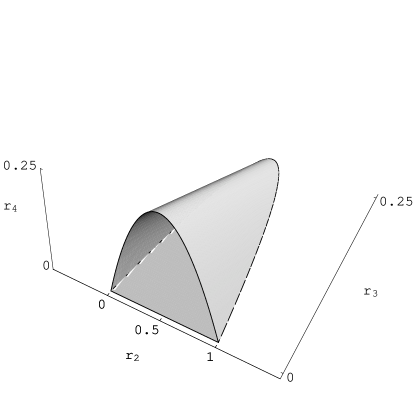
Figure 1: Section $\Xi$ of the four dimensional orbit space of Model 2 with the hyperplane of equation $\tilde{p}_{1}+\tilde{p}_{2}=1$.

Table 2: Orbit space characterization of strata $S$ of Model 3 and strata $\tilde{S}$ of Model 2. The $s_{i}$ are given in Eq. (11), $q=p_{1}p_{2}-p_{7}-p_{8}$, The relations defining the $\tilde{S}$’s are recovered setting $(p_{1},p_{2},p_{7},p_{8})=(\tilde{p}_{1},\tilde{p}_{2},\tilde{p}_{3},\tilde{p}_{4})$ and $p_{i}=0$ otherwise. Neighbouring strata are given, so that possible second order phase transitions can be easily identified.

Stratum	Defining relations	Boundary
$S^{(7)}\equiv\tilde{S}^{(4)}$	$s_{i}=0\leq q\,,i=1,\ldots,6\,;p_{j}\geq 0,\;j=3,4,7,8$	${\overline{S}^{(5)}}\,;\;{\overline{S}_{i}^{(4)}}\,,\;i=1,2,3$
	$p_{1}\,,p_{2}>0\,;\;\;(p_{1}+p_{2})p_{4}+p_{7}+p_{8}>0$
	$p_{3}\,(p_{1}+p_{2})+q>0$
	$p_{4}(p_{1}+p_{2})+p_{8}+(qp_{3}-p_{5}^{2})>0$
	$p_{7}(p_{1}+p_{2})+(qp_{3}-p_{5}^{2})>0$
$S^{(5)}\equiv\tilde{S}^{(3)}_{1}$	$s_{1}=p_{5}^{2}-q\,p_{3}=0=p_{i},\,\ i=7,9,10$	${\overline{S}_{2}^{(2)}}\,;{\overline{S}_{i}^{(3)}},\;i=1,2$
	$q\,,\;p_{i}\geq 0\,,\;i=1,2,3,4,8$
	$p_{1}+p_{2}>0\,,\;(p_{1}+p_{2})p_{4}+p_{8}>0$
	$q+(p_{1}+p_{2})p_{3}>0$
$S^{(4)}_{1}\equiv\tilde{S}^{(3)}_{2}$	$p_{5}^{2}-p_{3}\,q=0=p_{i},\ i=4,6,8,9,10$	${\overline{S}_{1}^{(3)}},{\overline{S}_{1}^{(2)}}$
	$p_{i}\geq 0,\ i=1,2,3$
	$p_{7}>0\,,\;q+p_{3}(p_{1}+p_{2})>0$
$S^{(4)}_{2}\equiv\tilde{S}^{(3)}_{3}$	$s_{1}=q=0=p_{i}\,,\;i=3,5,9,10\,;\;p_{7}>0\,$	${\overline{S}_{2}^{(3)}},{\overline{S}_{1}^{(2)}}$
	$p_{i}\geq 0\,,\;i=1,2,4\,;\;p_{4}(p_{1}+p_{2})+p_{8}>0$
$S^{(4)}_{3}$	$p_{i}=0,\ i=4,6,7,8,9,10$	${\overline{S}_{1}^{(3)}}$
	$p_{i}>0,\ i=1,2,3\,;\;p_{1}p_{2}p_{3}-p_{5}^{2}>0$
$S^{(3)}_{1}\equiv\tilde{S}^{(2)}_{1}$	$p_{5}^{2}-p_{1}p_{2}p_{3}=0=p_{i},\ i=4,6,7,8,9,10$	${\overline{S}_{i}^{(1)}},$ $i=1,2,3$
	$p_{i}\geq 0,\ i=1,2,3\,;p_{1}p_{2}+p_{3}(p_{1}+p_{2})>0$
$S^{(3)}_{2}\equiv\tilde{S}^{(2)}_{2}$	$s_{1}=q=0=p_{i},\ i=3,5,7,9,10$	${\overline{S}_{i}^{(1)}},$ $i=1,2,4$
	$p_{i}\geq 0,\ i=1,2\,;\;p_{1}p_{2}+p_{4}(p_{1}+p_{2})>0$
$S^{(2)}_{1}\equiv\tilde{S}^{(2)}_{3}$	$p_{7}-p_{1}p_{2}=p_{i}=0<p_{1}\;,p_{2},\;\;i\neq 1,2,7$	${\overline{S}_{1}^{(1)}}\,,\;{\overline{S}_{2}^{(1)}}$
$S^{(2)}_{2}$	$p_{i}=0,\ i\neq 3,4\,;\;0<p_{3}\;,p_{4}$	${\overline{S}_{3}^{(1)}}\,,\;{\overline{S}_{4}^{(1)}}$
$S^{(1)}_{1}\equiv\tilde{S}^{(1)}_{1}$	$p_{i}=0<p_{1},\;\ i\neq 1$	$S^{(0)}$
$S^{(1)}_{2}\equiv\tilde{S}^{(1)}_{2}$	$p_{i}=0<p_{2},\;\ i\neq 2$	$S^{(0)}$
$S^{(1)}_{3}$	$p_{i}=0<p_{3},\ i\neq 3$	$S^{(0)}$
$S^{(1)}_{4}$	$p_{i}=0<p_{4},\ i\neq 4$	$S^{(0)}$
$S^{(0)}\equiv\tilde{S}^{(0)}$	$p_{i}=0,\;\;\;1\leq i\leq 10$

Table 3: Symmetries of the strata $S$ of Model 3 and $\tilde{S}$ of Model 2. The group $\mathrm{U}_{1}^{\mathrm{e.m.}}$ is defined as in Table (1), and $\alpha=\mathrm{e}^{\mathrm{i}\pi(T_{3}-Y/2)}$. Symmetries are specified by a representative element of the conjugacy class of isotropy subgroups. Finite groups are defined through their generators between brackets. For each stratum, a field configuration with the same symmetry is supplied (typical point). The fields are represented by their real components: $\Phi_{1}^{\mathrm{T}}=(\phi_{1}+\mathrm{i}\phi_{2},\phi_{3}+\mathrm{i}\phi_{4})$, $\Phi_{2}^{\mathrm{T}}=(\phi_{5}+\mathrm{i}\phi_{6},\phi_{7}+\mathrm{i}\phi_{8})$, $F=\phi_{9}+\mathrm{i}\phi_{10}$ and $H=\phi_{11}$, where the $\phi_{i}$’s are generic non zero values.

Stratum	Symmetry	Typical point $\phi$
$S^{(7)}\equiv\tilde{S}^{(4)}$	$\{1\!\!1\}$	$(\phi_{1},0,\phi_{3},\phi_{4},0,0,\phi_{7},0,\phi_{9},\phi_{10},\phi_{11})$
$S^{(5)}\equiv\tilde{S}^{(3)}_{1}$	$\{\hat{\iota}\,K\}$	$(\phi_{1},0,\phi_{3},0,0,0,0,\phi_{8},\phi_{9},0,\phi_{11})$
$S^{(4)}_{1}\equiv\tilde{S}^{(3)}_{2}$	$\{K\}$	$(\phi_{1},0,\phi_{3},0,0,0,\phi_{7},0,0,\phi_{10},0)$
$S^{(4)}_{2}\equiv\tilde{S}^{(3)}_{3}$	U${}_{1}^{\mathrm{e}.m.}$	$(0,0,\phi_{3},\phi_{4},0,0,\phi_{7},0,0,0,\phi_{11})$
$S^{(4)}_{3}$	$\{\alpha\,\hat{\iota}\}$	$(\phi_{1},0,0,0,0,0,\phi_{7},0,\phi_{9},\phi_{10},0)$
$S^{(3)}_{1}\equiv\tilde{S}^{(2)}_{1}$	$\{\alpha\,\hat{\iota},K\}$	$(\phi_{1},0,0,0,0,0,\phi_{7},0,0,\phi_{10},0)$
$S^{(3)}_{2}\equiv\tilde{S}^{(2)}_{2}$	U${}_{1}^{\mathrm{e}.m.}\times\,\{\hat{\iota}\,K\}$	$(0,0,\phi_{3},0,0,0,0,\phi_{8},0,0,\phi_{11})$
$S^{(2)}_{1}\equiv\tilde{S}^{(2)}_{3}$	U${}_{1}^{\mathrm{e}.m.}\times\{K\}$	$(0,0,\phi_{3},0,0,0,\phi_{7},0,0,0,0)$
$S^{(2)}_{2}$	SU${}_{2}\times\{\hat{\iota}\,K\}$	$(0,0,0,0,0,0,0,0,\phi_{9},0,\phi_{11})$
$S^{(1)}_{1}\equiv\tilde{S}^{(1)}_{1}$	U${}_{1}^{\mathrm{e}.m.}\,\times\{\hat{\iota},K\}$	$(0,0,\phi_{3},0,0,0,0,0,0,0,0)$
$S^{(1)}_{2}\equiv\tilde{S}^{(1)}_{2}$	U${}_{1}^{\mathrm{e}.m.}\times\{e^{i\pi Y}\,\hat{\iota},K\}$	$(0,0,0,0,0,0,\phi_{7},0,0,0,0)$
$S^{(1)}_{3}$	SU${}_{2}\times\{\hat{\iota}\,K\,,\mathrm{e}^{\mathrm{i}\pi Y/2}\,\hat{\iota}\}$	$(0,0,0,0,0,0,0,0,\phi_{9},0,0)$
$S^{(1)}_{4}$	$(\mathrm{SU}_{2}\times\mathrm{U}_{1})/{\mathbb{Z}}_{2}\times\{\hat{\iota}\,K\}$	$(0,0,0,0,0,0,0,0,0,0,\phi_{11})$
$S^{(0)}\equiv\tilde{S}^{(0)}$	$(\mathrm{SU}_{2}\times\mathrm{U}_{1})/{\mathbb{Z}}_{2}\,\times\{\hat{\iota}\,,\;K\}$	$(0,0,0,0,0,0,0,0,0,0,0)$

We shall consider two different dynamical versions of Model 2, a complete non-renormalizable and an incomplete renormalizable one.

4.1 Model $2_{1}$: A complete non-renormalizable version of Model 2

For the reasons explained in the Introduction, let us now ignore the renormalizability condition. Then, the simple potential defined in (6), with the ${\tilde{p}}_{i}$’s specified in (7) replacing the $p_{i}$’s, is already sufficient (despite its being not the most general $G$-invariant eighth-degree polynomial), to make observable all the allowed phases. It admits, in fact, a stable minimum in each of the strata ${\tilde{S}}$ listed in Tables 2 and 3, for suitable values of the $a_{i}$’s, as can be easily realized, with the help of Figure 1, conveniently modifying the geometrical arguments exploited to determine the observable phases of Model 1. The transformation in Eq. (8) leads to a four dimensional semialgebraic set which, contrary to $\Xi$, is not convex, but, fortunately, like $\Xi$, has no intruding cusps. In particular, for $A\propto 1\!\!1$ let us denote by $\Omega$ the image, $\eta=p({\mathbb{R}}^{8})$, of the orbit space in the space of the $\eta_{i}$’s. Then, if $\eta$ is within or near enough to $\Omega$, there is only one local minimum of the potential (the absolute minimum) at the point $\tilde{p}$ of the orbit space which is at the shortest distance from $\eta$.

The above statements have been checked analytically; in particular, we have determined the superposition regions in the $\eta$ parameter space, where two local minima of potential (6) can co-exist in two different symmetry strata [14]. Such a situation is quite important from a phenomenological point of view, since it can lead, even at the classical level, to first order phase transitions [9].

4.2 Model $2_{2}$: An incomplete renormalizable version of Model 2

Let us now, in the frame of symmetries of Model 2, chose the Higgs potential as the most general, bounded below invariant polynomial of degree four:

$$\widehat{V}(\tilde{p})=\sum_{i,j=1}^{2}\,A_{ij}\,\tilde{p}_{i}\,\tilde{p}_{j}+\sum_{i=1}^{4}\,a_{i}\,\tilde{p}_{i},$$ (9)

where all the parameters are real and $A_{12}=A_{21}$.

As stated in [7], since there are no relations among the basic invariants and the potential is linear in those of degree four, its local minima can only sit on the boundary of the orbit space, for general values of the $a_{i}$’s. A detailed calculation shows that there can be stationary points of the potential in the strata of dimension $\geq 3$ only if the $a_{i}$’s satisfy particular conditions: $a_{3}=a_{4}=0$, $a_{4}=0$, $a_{3}=0$ and $a_{3}=a_{4}$, respectively, for the strata $\tilde{S}^{(4)}$, $\tilde{S}^{(3)}_{1}$, $\tilde{S}^{(3)}_{2}$ and $\tilde{S}^{(3)}_{3}$. These conditions reduce to zero the measures of the regions of stability of the corresponding phases, in the space of the parameters $a_{i}$. So, there will not be stable phases associated to the strata of dimension $\geq 3$. As a consequence, it is impossible to generate spontaneous $CP$ violation in the model. The general problem of spontaneous $CP$ breaking in two-Higgs doublet models will be faced in a forthcoming paper [9].

We can conclude that Model $2_{2}$ is renormalizable, but it is incomplete. In tree-level approximation, the phases associated to the strata of dimension $\geq 3$ have zero probability to be observed in nature.

5 Model 3

The comparison of models $2_{1}$ and $2_{2}$ suggests a way to make observable all the phases allowed by the symmetry of Model 2, without changing the symmetry group $G=(\mathrm{SU}_{2}\times\mathrm{U}_{1})/{\mathbb{Z}}_{2}\,\times\{\hat{\iota}\,,\,K\}$. If some of the basic SU₂ invariant polynomials which have been used to build up the basic invariants of Model 2 are considered as independent singlet scalar fields, the potential of Model $2_{1}$, written in terms of the new fields, can take on a renormalizable form. Here, the new SU₂ singlet scalar fields are added only as a technical trick, but they could be thought of as describing bound states of the original scalar doublets. The introduction of additional scalar fields in a model modifies the symmetry and might enlarge the number of allowed phases. However, one can get rid of possible new phases, by making them dynamically unattainable.

Let us just analyze one of these possibilities, that we shall call Model 3, which is obtained from Model 2 by adding a complex, hypercharge 2 singlet $F$ and a real, hypercharge 0 singlet $H$ with transformation rules $(F,H)\rightarrow(-F,-H)$ and, respectively, $(F,H)\rightarrow(-F^{*},-H)$ under transformations induced by $\hat{\iota}$ and $K$.

The following set of invariants yields a MIB in the present case:

$${\begin{array}[]{l}p_{1}=\tilde{p}_{1},\ \ p_{2}=\tilde{p}_{2},\ \ p_{3}=|F|^{2},\ \ p_{4}=H^{2},\ \ p_{5}=\mathrm{Re}[\Phi_{2}^{\mathrm{T}}\sigma_{2}\Phi_{1}\,F^{*}],\\ p_{6}=\mathrm{Im}\left[\Phi_{2}^{\dagger}\Phi_{1}\right]H,\;p_{7}=\tilde{p}_{3},\;p_{8}=\tilde{p}_{4},\;p_{9}=H\,\mathrm{Re}\left[\Phi_{2}^{\dagger}\Phi_{1}\right]\mathrm{Im}[\Phi_{2}^{\mathrm{T}}\sigma_{2}\Phi_{1}\,F^{*}],\\ p_{10}=\mathrm{Re}\left[\Phi_{2}^{\dagger}\Phi_{1}\right]\mathrm{Im}\left[\Phi_{2}^{\dagger}\Phi_{1}\right]\mathrm{Im}[\Phi_{2}^{\mathrm{T}}\sigma_{2}\Phi_{1}\,F^{*}],\end{array}}$$ (10)

where $\tilde{p}_{j}$, $j=1,\dots,4$ are defined in (7).

The elements of the MIB have degrees $\{2,2,2,2,3,3,4,4,6,7\}$ and are related by the syzygies $s_{i}=0$, $1\leq i\leq 6$:

$${\begin{array}[]{rcl}s_{1}&=&p_{6}^{2}-p_{4}\,p_{8},\ s_{2}=p_{9}^{2}-p_{4}\,p_{7}\left(p_{3}q-p_{5}^{2}\right),\ s_{3}=p_{10}^{2}-p_{7}\,p_{8}\left(p_{3}q-p_{5}^{2}\right),\\ s_{4}&=&p_{6}\,p_{9}-p_{4}\,p_{10},\ s_{5}=p_{6}\,p_{10}-p_{8}\,p_{9},\ s_{6}=p_{9}\,p_{10}-p_{6}\,p_{7}\left(p_{3}q-p_{5}^{2}\right),\end{array}}$$ (11)

where $q=p_{1}\,p_{2}-p_{7}-p_{8}$. Only three of the syzygies are independent. Therefore, the orbit space is a semialgebraic subset of the seven dimensional algebraic variety defined by the set of equations $s_{i}=0$, $i=1,\dots,6$. As usual, the orbit space and its stratification can be determined from rank and positivity conditions of the $\widehat{P}(p)$-matrix associated to the MIB defined in (10). The results are reported in Tables 2 and 3. As expected, four new phases (i.e.: $S^{(4)}_{3}$, $S^{(2)}_{2}$, $S^{(1)}_{3}$, $S^{(1)}_{4}$), that were not allowed by the symmetry of Model 2, are now allowed.

The most general invariant polynomial of degree four in the scalar fields of the model can be written in terms of the following polynomial $\widehat{V}(p)$ in the $p_{i}$’s with degree $\leq 4$:

$${\widehat{V}(p)=\sum_{i=1}^{8}\,a_{i}\,p_{i}+\sum_{i,j=1}^{4}\,A_{ij}\,p_{i}\,p_{j}.}$$ (12)

The conditions for a stationary point of $\widehat{V}(p)$ in a given stratum are obtained from equation (4) and the explicit form of the $f_{\alpha}(p)$ can be read from Table 2.

The high dimensionality of the orbit space prevents, in this case, a simple geometric determination of the conditions assuring the existence of a stable local minimum on a given stratum and a complete analytic solution of these conditions is impossible, since high degree polynomial equations are involved. Despite this, using convenient majorisations, we have been able to prove [14] that all the phases allowed by the symmetry of Model 2 (which are, obviously, also allowed by the symmetry of Model 3) are observable in Model 3. The result holds in the following strong sense: For each phase of symmetry $(H)$ allowed by the symmetry of Model 2, we have analytically determined an 8-dimensional open semialgebraic set ${R}_{H}$ in the space of the coefficients $a=(a_{1},\dots,a_{8})$ and an open neighborhood ${I}_{H}$ of the four dimensional unit matrix, such that, for all $a\in{R}_{H}$ and $A\in{I}_{H}$, the potential $\widehat{V}(p(\phi))$, defined through (12), has a stable absolute minimum in the stratum of Model 3 with symmetry $(H)$. Moreover, for $a\in{R}_{H}$ and $A\in{I}_{H}$, the potential has no local minimum in the strata of Model 3 corresponding to phases not allowed in Model 2. In particular:

1. All the allowed phases of Model 3 turn out to be observable with the potential defined in (12), but for the phase corresponding to the stratum $S^{(4)}_{3}$ (a local minimum lies in this stratum only if $a_{5}=0$, which means that the minimum is unstable), so that Model 3, which is renormalizable, is not far from being also complete;

2. For $A=1\!\!1$, a stable local minimum can be found only in the strata of Model 3 corresponding to allowed phases of Model 2, provided that $a_{1}+a_{2}<0$ and $a_{3}\,a_{4}>0$.

A complete specification of the sets ${R}_{H}$ and ${I}_{H}$ would be too long to be given in this Letter and will be reported elsewhere [14].

Let us conclude by stressing that Model 3 could be relevant in the study of electro-weak baryogenesis: $CP$ violation is achieved in phase $S^{(4)}_{2}$, so it is interesting to examine the possibility of first order phase transitions to more symmetrical phases [9].

References

- [1] S. J. Glashow, Partial symmetries of weak interactions, Nucl. Phys. 22 (1961) 579–588; A. Salam, in: N. Svartholm, Almquist and Wikselt, eds., Elementary Particle Theory (Stockolm, 1969) 367; S. Weinberg, A Model of Leptons, Phys. Rev. Lett. 19 (1967) 1264–1266.
- [2] M. Sher, Electroweak Higgs potential and vacuum stability, Phys. Rep. 179 (1989) 273–418.
- [3] J. Gunion, H. Haber and G. Kane, S. Dawson, The Higgs Hunter’s Guide (Perseus Publishing, Cambridge MA, 1990).
- [4] J. Choi and R.R. Volkas, Real Higgs singlet and the electroweak phase transition in the standard model, Phys. Lett. B 317 (1993) 385–391.
- [5] T. Gherghetta and A. Pomarol, The Standard Model Partly Supersymmetric, preprint hep-ph/0302001.
- [6] We are not interested in possible isostructural phase transitions taking place when a continuous variation of the ’s induces a discontinous displacement (a jump) of the location of the minimum to a different point of the same stratum.
- [7] M. Abud and G. Sartori, The geometry of orbit space and natural minima of Higgs potentials, Phys. Lett. B 104, 147–152 (1981) and The geometry of spontaneous symmetry breaking, Ann. Phys. 150, 307 (1983); see also G. Sartori, Geometric Invariant Theory: A Model-Independent Approach to Spontaneous Symmetry and/or Supersymmetry breaking, La Rivista del Nuovo Cimento 14, 1–120 (1991) and references therein.
- [8] Yu.M. Gufan, O.D. Lalakulich, G. Sartori and G.M. Vereshkov, Evolution of the Universe in two-Higgs doublets Standard Models, in: D. Bambusi, M. Cadoni and G. Gaeta eds., Proceedings of Symmetry and Perturbation Theory 2001 (World Scientific, Singapore, 2002 - ISBN 981-02-4793-1) 78–91.
- [9] A. Masiero, G. Sartori and G. Valente, in preparation.
- [10] The invariant can always be included in a MIB and, in this case, the image in of the unit sphere of is the hyperplane of equation .
- [11] H. Georgi and A. Pais, Vacuum symmetry and the pseudo-Goldstone phenomenon, Phys. Rev. D 12 (1975) 508–512.
- [12] The statement holds at the classical level, i.e. until no radiative or finite temperature corrections are introduced in the potential.
- [13] S. Weinberg, Gauge Theory of CP Nonconservation, Phys. Rev. Lett. 37 (1976) 657–661.
- [14] G. Sartori and G. Valente, in preparation.