Soft parton radiation in polarized vector boson production:
theoretical issues

Abstract

Accurate measurement of spin-dependent parton distributions in production of electroweak bosons with polarized proton beams at the Relativistic Heavy Ion Collider depends on good understanding of QCD radiation at small transverse momenta $q_{T}$ of vector bosons. We present a theoretical formalism for small-$q_{T}$ resummation of the cross sections for production of $\gamma^{*}$, $W^{\pm}$, and $Z^{0}$ bosons, with the subsequent decay of these bosons into lepton pairs, for arbitrary longitudinal polarizations of the proton beams.

I Introduction

The commissioning of polarized proton beams with energies from 100 to 250 GeV at the Relativistic Heavy Ion Collider (RHIC) Boer et al. (2001) has started a new stage in physics of spin-dependent collisions. In particular, measurement of spin-dependent parton distribution functions (PDFs) will be the top priority in the experiments with longitudinal polarization. So far, these spin-dependent counterparts of the unpolarized PDFs were constrained only by the lepton-nucleon deep inelastic scattering (DIS) data Ashman et al. (1988, 1989); Adeva et al. (1998); Anthony et al. (1996); Abe et al. (1998, 1997); Anthony et al. (1999); Ackerstaff et al. (1997); Airapetian et al. (1998), which concentrates at relatively small momentum transfers ($Q^{2}\sim 1\mbox{\, GeV}^{2}$). In contrast, RHIC will explore the spin-dependent PDFs in a much larger range of $Q^{2}$ and using a variety of spin-dependent particle reactions, including production of Drell-Yan lepton pairs and resonant production of $W^{\pm}$ and $Z^{0}$ bosons Bunce et al. (2000).

Vector boson production (VBP) with polarized hadron beams, which proceeds through annihilation of a quark and antiquark at the Born level, is the most natural candidate to probe spin-dependent quark polarizations Close and Sivers (1977); Bourrely et al. (1980); Craigie et al. (1983). Furthermore, in $pp$ collisions the Born level cross sections are sensitive to the distributions of sea quarks. In this sense, VBP complements production of jets, pions, and heavy quark flavors, which primarily probe the gluon distribution. No wonder that extensive bibliography is dedicated to spin-dependent production of Drell-Yan pairs Ratcliffe (1983); Richter-Was and Szwed (1985); Cheng and Lai (1990); Bourrely et al. (1991); Weber (1992); Mathews and Ravindran (1992); Chiappetta et al. (1993); Kamal (1996); Gehrmann (1997); Kumano:1999bt ; Dressler:1999zv ; Gluck:2000ek ; Ravindran et al. (2002); Kodaira:2003tq and massive electroweak bosons Chiappetta and Soffer (1985); Weber (1993); Bourrely and Soffer (1994, 1993); Nadolsky (1995); Bourrely and Soffer (1995); Kamal (1998); Gehrmann (1998); Gluck:2000ek .

The production of $W^{\pm}$ bosons presents a particularly interesting opportunity to learn about the quark spin structure due to the maximal violation of space-reflection parity in the $q\bar{q}W$ coupling and non-trivial mixing of the quark flavors through the Cabibbo-Kobayashi-Maskawa (CKM) matrix Cabibbo (1963); Kobayashi and Maskawa (1973). While the former feature allows non-vanishing single-spin cross section asymmetries (which are simpler than the parity-conserving double-spin asymmetries), the latter feature facilitates the study of the flavor dependence of the sea quark PDFs. The issue of flavor symmetry breaking in the polarized quark sea was brought in the limelight recently by the results on semi-inclusive hadroproduction in spin-dependent DIS by HERMES Collaboration Ackerstaff et al. (1999). In that measurement, the issues of higher-order and higher-twist corrections are an important consideration due to small values of $Q^{2}$. At the same time, $W$ boson production at RHIC has a potential to pin down the quark sea flavor structure at large $Q^{2}$, i.e., at energies where perturbative quantum chromodynamics (PQCD) is truly valid.

The original method Bland (2000); Bunce et al. (2000) for the measurement of polarized PDFs in $W$ boson production at RHIC relies on the reconstruction of the spin-dependent distribution $d\sigma/dy$ over the rapidity $y$ of the $W$ bosons. The method is based on the observation that the Born level single-spin asymmetry of $d\sigma/dy$ is described by a simple theoretical expression, which further reduces to the ratio $\Delta q(x)/q(x)$ of the polarized and unpolarized PDFs when the absolute value of $y$ is large. Unfortunately, the application of this method is obstructed by specifics of the detection of the $W^{\pm}$ bosons at RHIC. Since neither of RHIC detectors controls the energy balance in particle reactions, the energy and momentum of the neutrino in the decay are completely unknown, so that the information about the momentum of the $W$ boson is incomplete. As a result, the determination of the rapidity $y$ of the $W$ boson from the observation of just one charged lepton is generally impossible.

It can be shown that the ambiguity in the reconstruction of $y$ reduces to the uncertainty in the knowledge of the transverse momentum $q_{T}$ of the $W$ boson Bunce et al. (2000). If $q_{T}$ were known exactly, the rapidity $y$ of the $W$ boson can be derived (up to a two-fold ambiguity) from the measured rapidity $y_{\ell}$ and transverse momentum $p_{T\ell}$ of the charged lepton (see the accompanying paper Nadolsky and Yuan (2003) for more details on this reconstruction method). For instance, if all $W$ bosons were produced through the Born process $q\bar{q}\rightarrow W$, the transverse momentum $q_{T}$ would be zero, and the correct solution for $y$ can be chosen statistically for the leptons with large absolute values of the lepton rapidity $y_{\ell}$, i.e., escaping near the beam pipe direction.

In reality, the $W^{\pm}$ bosons carry a non-zero transverse momentum due to QCD radiation, with the most probable magnitude in the unpolarized case of about 2 GeV. Most of the $W^{\pm}$ bosons obtain a non-zero $q_{T}$ through the radiation of soft and collinear partons, which cannot be approximated by finite-order perturbative calculations. Since the power series in the strong coupling $\alpha_{S}$ does not converge in the small-$q_{T}$ region, summation of dominant logarithmic terms through all orders of this series is needed. This all-order summation can be realized with the help of the methods that were studied in a substantial detail Dokshitzer et al. (1978); Parisi and Petronzio (1979); Altarelli et al. (1979); Collins and Soper (1981, 1982); Collins et al. (1985); Davies et al. (1985); Arnold and Kauffman (1991); Balazs and Yuan (1997); Ladinsky and Yuan (1994); Ellis et al. (1997); Ellis and Veseli (1998); Landry et al. (2001); Qiu and Zhang (2001a, b); Kulesza and Stirling (2001); Landry et al. (2002) in the unpolarized case. Note, however, that the properties of the multiple parton radiation depend on the spin of the initial hadrons. The spin dependence of the collinear radiation off the external parton lines can be seen from an explicit calculation. An additional spin dependence can be contributed by the unknown nonperturbative dynamics of strong interactions at large distances. Thus, conclusions about the nature of the multiple parton radiation in the polarized hadronic collisions cannot be inferred from the unpolarized case, and an additional study is required to estimate the spin dependence of such radiation under the RHIC conditions.

The main goal of this paper is to provide a theoretical framework for such a study. We present a complete formalism for resummation in VBP with the proton beams of an arbitrary longitudinal polarization. Furthermore, we explicitly account for the decay of the vector bosons into the observed leptons, which is important because of the complicated geometry of RHIC detectors. The results are derived at a one-loop level of PQCD, and the summation of large logarithms is performed with the help of the impact parameter resummation technique Collins et al. (1985). The detailed discussion of this lepton-level resummation formalism in the unpolarized case can be found in Ref. Balazs and Yuan (1997). The theoretical results are presented for arbitrary couplings of the vector boson, which makes the results of this paper also applicable to lepton pair production mediated by photons or $Z^{0}$ bosons. Our eventual product is a numerical program for Monte-Carlo integration of fully differential resummed cross sections in the presence of experimental cuts. In the accompanying paper Nadolsky and Yuan (2003), we present numerical results for the single-spin asymmetries in $W$ boson production and estimate the sensitivity of these asymmetries to different models of polarized PDFs.

To review the already available literature, we note that the finite-order asymmetries of order ${\mathcal{O}}(\alpha_{S})$ in the Drell-Yan process are currently available for distributions in full lepton pair momentum Weber (1992), invariant mass Kamal (1996), and rapidity Gehrmann (1997). Analogous distributions for $W$ boson production were published in Refs. Kamal (1998); Gehrmann (1998); Weber (1993). Recently, the ${\mathcal{O}}(\alpha_{S}^{2})$ fully differential distributions of the Drell-Yan pairs were obtained in Ref. Ravindran et al. (2002). Furthermore, Refs. Weber (1992, 1993) presented the ${\mathcal{O}}(\alpha_{S})$ resummed single- and double-spin cross sections in the narrow width approximation, and the ${\mathcal{O}}(\alpha_{S})$ Sudakov factor was explicitly demonstrated to be independent from the polarization of the proton beams. Note that most of the above publications (with the exception of the forward-backward asymmetry in Ref. Kamal (1998) and polar angle distribution of the Drell-Yan leptons in the lab frame in Ref. Kodaira:2003tq ) discuss the behavior of the whole lepton pair, rather than the distributions of the individual leptons.

In this paper, we go beyond the previous results in several aspects. First, we present the fully differential finite-order and resummed cross sections for the decaying electroweak vector bosons, i.e., we completely account for the spin correlations between the hadronic subsystem and leptonic final state. In other words, the cross sections in this work are fully differential in the individual lepton momenta, rather than in the momentum of the lepton pair. These cross sections are implemented in a Monte-Carlo integration program. Such lepton-level analysis requires calculation of several additional angular structure functions, which do not contribute in the narrow width approximation. Furthermore, the $q_{T}$ resummation is needed not only for the parity-conserving angular function $1+\cos^{2}\theta$, which contributes to the boson-level cross section, but also for the parity-violating angular function $2\cos\theta$, which affects the angular distributions of the decay products. The calculation for the parity-violating term $2\cos\theta$ is substantially more complex, because it involves a large number of $\gamma_{5}$ matrices (and Levi-Civita tensors) coming from both spin projection operators and axial couplings of the electroweak Lagrangian. In contrast, the parity-conserving term $1+\cos^{2}\theta$ depends on $\gamma_{5}$ matrices and Levi-Civita tensors from the spin projection operators only.

It is well known that special care is needed to deal with the $\gamma_{5}$ matrices in $n\neq 4$ dimensions. In order to tackle this issue efficiently, we have evaluated the $n$-dimensional cross sections using the dimensional reduction method Siegel (1979); Schuler et al. (1987); Korner and Tung (1994). We then converted our results to the conventional $\overline{MS}$ factorization scheme, which utilizes dimensional regularization ’t Hooft and Veltman (1972); Breitenlohner and Maison (1977). From our calculation, we have found that the spin-dependent resummed cross-sections in Weber (1992, 1993) could not be used with the existing parametrizations of the polarized PDFs in the $\overline{MS}$ scheme, due to the different factorization scheme used in those papers. In addition, Ref. Weber (1993) has used an unconventional normalization for the $n$-dimensional single-spin cross section in the $qG$ channel. The present work has paid a special attention to rectify those inconsistencies and obtain the hard cross sections compatible with the existing phenomenological PDF parametrizations in the $\overline{MS}$ scheme.

The paper has the following structure. In Section II, we introduce the notations for the kinematical variables and spin-dependent cross sections. Section III discusses the regularization of cross section singularities by continuation of observables to $n\neq 4$ dimensions, as well as the treatment of the $\gamma_{5}$ matrices. In Section  IV, we present in detail the ${\mathcal{O}}(\alpha_{S})$ finite-order and resummed cross sections. Section V contains the summary of our results and conclusions. The appendix contains the expressions for all structure functions that contribute to the lepton-level ${\mathcal{O}}(\alpha_{S})$ cross sections.

II Notations

II.1 Kinematical variables

We discuss inclusive production of a lepton pair $A(p_{A})+B(p_{B})\rightarrow V^{*}(q)+X\rightarrow\ell_{1}(l_{1})+\bar{\ell}_{2}(l_{2})+X$ mediated by a virtual vector boson $V$. Our notations for the particle momenta and helicities in this process are shown in Fig. 1.

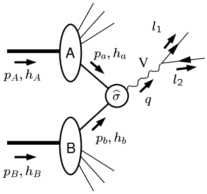
Figure 1: Notations for the momenta and helicities of the participating particles.

The momentum $q^{\mu}$ of $V$ can be conveniently parametrized by the invariant mass $Q$, rapidity $y$, and transverse momentum $q_{T}$ of the vector boson in the laboratory frame. We have

$$Q^{2} \equiv q^{\mu}q_{\mu};$$ (1)

$$y \equiv \frac{1}{2}\ln\frac{q_{+}}{q_{-}};$$ (2)

$$q_{T}^{2} \equiv -q_{t}^{\mu}q_{t\mu},$$ (3)

where $q_{t}^{\mu}$ is the component of the momentum $q^{\mu}$ that is orthogonal (in the relativistic sense) to the momenta $p_{A}^{\mu}$ and $p_{B}^{\mu}$:

$$q_{t}^{\mu}\equiv q^{\mu}-\frac{(p_{A}\cdot q)}{(p_{A}\cdot p_{B})}p_{B}^{\mu}-\frac{(p_{B}\cdot q)}{(p_{A}\cdot p_{B})}p_{A}^{\mu}.$$ (4)

For any vector $n^{\mu}$, the “plus” and “minus” components are defined as $n_{\pm}\equiv\left(n^{0}\pm n^{3}\right)/\sqrt{2}$.

It will be useful to introduce the hadronic and partonic Mandelstam invariants, defined by

$$s = (p_{A}+p_{B})^{2};$$ (5)

$$t = (p_{A}-q)^{2};$$ (6)

$$u = (p_{B}-q)^{2};$$ (7)

$$\widehat{s} = (p_{a}+p_{b})^{2};$$ (8)

$$\widehat{t} = (p_{a}-q)^{2};$$ (9)

$$\widehat{u} = (p_{b}-q)^{2}.$$ (10)

A caret denotes quantities at the parton level. They are defined in terms of the parton momenta $p_{a}^{\mu}\equiv\xi_{a}p_{A}^{\mu},$ $p_{b}^{\mu}\equiv\xi_{b}p_{B}^{\mu},$ where $\xi_{a}$ and $\xi_{b}$ are the light-cone momentum fractions, which satisfy the constraints $x_{A}\leq\xi_{a}\leq 1,$ $x_{B}\leq\xi_{b}\leq 1$, with $x_{A,B}\equiv Qe^{\pm y}/\sqrt{s}$. Throughout the discussion, all hadron masses are neglected.

Our discussion will use two coordinate frames. The first frame is the laboratory frame, or the center-of-mass frame of the initial proton beams. The second frame is a special rest frame of the produced vector boson (Collins-Soper frame Collins and Soper (1977)), in which the axis $Oz$ bisects the angle between the vectors ${\bf p}_{A}$ and $-{\bf p}_{B}$, where ${\bf p_{A}}$ are ${\bf p_{B}}$ are the initial hadrons’ momenta in this frame. The coordinate transformation from the lab frame to the Collins-Soper frame involves a boost in the direction of motion of $V$ and a rotation around the $Oy$ axis (see Appendix A in Balazs and Yuan (1997) for the explicit coordinate transformation matrix). The components of the momenta $p_{A}^{\mu}$ and $p_{B}^{\mu}$ in the Collins-Soper frame are

$$p_{A,B}^{\mu}=\sqrt{\frac{s}{2}}\left(\frac{q_{\mp}}{Q},-\frac{q_{\mp}q_{T}}{M_{T}Q},0,\pm\frac{q_{\mp}}{M_{T}}\right),$$ (11)

where $M_{T}$ is the transverse mass of the vector boson, $M_{T}\equiv\sqrt{Q^{2}+q_{T}^{2}}.$ The momenta $l_{1}^{\mu}$ and $l_{2}^{\mu}$ of the final-state leptons in this frame are

$$l_{1}^{\mu} = \frac{Q}{2}\Biggl{(}1,\sin\theta\cos\varphi,\sin\theta\sin\varphi,\cos\theta\Biggr{)},$$ (12)

$$l_{2}^{\mu} = \frac{Q}{2}\Biggl{(}1,-\sin\theta\cos\varphi,-\sin\theta\sin\varphi,-\cos\theta\Biggr{)}.$$ (13)

Instead of using $l_{1}^{\mu}$ and $l_{2}^{\mu}$ directly, it is convenient to operate with their linear combinations,

$$q^{\mu}=l_{1}^{\mu}+l_{2}^{\mu}=\Biggl{(}Q,0,0,0\Biggr{)}$$ (14)

and

$$l_{12}^{\mu}\equiv l_{1}^{\mu}-l_{2}^{\mu}=Q\Biggl{(}0,\sin\theta\cos\varphi,\sin\theta\sin\varphi,\cos\theta\Biggr{)}.$$ (15)

While $q^{\mu}$ describes the motion of the lepton pair as a whole, $l_{12}^{\mu}$ specifies the motion of the individual leptons in the decay of the vector boson. To separate the dynamics of vector boson production from the dynamics of vector boson decay, we decompose the lepton-level cross section in a sum over the functions $A_{\rho}(\theta,\varphi)$ of the angles $\theta$ and $\varphi$ in the Collins-Soper frame:

$$\frac{d\sigma}{dQ^{2}dydq_{T}^{2}d\Omega}=\sum_{\rho=-1}^{4}{}^{\rho}T(Q^{2},y,q_{T}^{2})A_{\rho}(\theta,\varphi).$$ (16)

In this equation, $d\Omega\equiv d\cos\theta\,d\varphi$ denotes an element of the solid angle in the Collins-Soper frame. ${}^{\rho}T(Q^{2},y,q_{T}^{2})$ is the structure function corresponding to the angular function $A_{\rho}(\theta,\varphi)$. For an arbitrary chirality of the electroweak couplings, VBP at ${\mathcal{O}}(\alpha_{S})$ receives contributions from six angular functions $A_{\rho}(\theta,\varphi)$:

$$A_{-1}\equiv 1+\cos^{2}\theta; A_{0}\equiv\frac{1}{2}(1-3\cos^{2}\theta);$$

$$A_{1}\equiv\sin 2\theta\cos\varphi; A_{2}\equiv\frac{1}{2}\sin^{2}\theta\cos 2\varphi;$$

$$A_{3}\equiv 2\cos\theta; A_{4}\equiv\sin\theta\cos\varphi.$$ (17)

The angular function $A_{-1}(\theta,\varphi)$ is also sometimes denoted as ${L}_{0}(\theta,\varphi)$ (see, for instance, Ref. Balazs and Yuan (1997)). It will be shown below that the structure functions ${}^{-1}T,$ ${}^{0}T,$ ${}^{1}T,$ and ${}^{2}T$ are generated by the vector part of the electroweak current. On the other hand, the structure functions ${}^{3}T$ and ${}^{4}T$ are generated by the axial part of the electroweak current. This feature leads to the following important consequence. When the cross section is integrated over the complete solid angle $\Omega$ of the lepton decay (as, e.g., in the calculation of a boson-level cross section), all angular functions except $A_{-1}$ are integrated out. The resulting cross section is sensitive only to the vector part of the electroweak current, so that, for instance, the $W$ boson cross section can be straightforwardly derived from the Drell-Yan pair cross section. On the other hand, if one is interested in the angular distributions of the final-state leptons, the axial part of the electroweak current cannot be ignored. In that case, additional care is needed in the calculation of the parity-violating structure functions ${}^{3}T$ and ${}^{4}T,$ which are affected by the $\gamma_{5}$ matrices from both the spin projection operators and electroweak couplings.

II.2 Polarized cross sections

We now introduce the special notations that will allow us to write the cross sections for arbitrary proton polarizations in a compact form. Let the polarized protons $A$ and $B$ have helicities $h_{A}$ and $h_{B}$, respectively. The allowed values are $+1$ for the right-handed helicities and $-1$ for the left-handed helicities. The cross section for this combination of the helicities is denoted as $\sigma^{h_{A}h_{B}}$. For brevity, the superscripts of $\sigma^{h_{A}h_{B}}$ will only show the signs of the helicities; that is, $\sigma^{+1,+1}\equiv\sigma^{++},$ $\sigma^{+1,h_{B}}\equiv\sigma^{+h_{B}},$ etc.

The following combinations of the helicity cross sections will be called “the cross sections that are unpolarized (U) or polarized (P) on the side of the proton $A$”:

$$\sigma^{(U,h_{B})} \equiv \sigma^{+h_{B}}+\sigma^{-h_{B}},$$ (18)

$$\sigma^{(P,h_{B})} \equiv \sigma^{+h_{B}}-\sigma^{-h_{B}}.$$ (19)

Similarly, “the cross sections that are unpolarized (polarized) on the side of the of the proton $B$” are

$$\sigma^{(h_{A},U)} \equiv \sigma^{h_{A}+}+\sigma^{h_{A}-},$$ (20)

and

$$\sigma^{(h_{A},P)} \equiv \sigma^{h_{A}+}-\sigma^{h_{A}-},$$ (21)

respectively.

Next, we introduce the unpolarized, single-spin, and double-spin cross sections $\sigma^{(U,U)},$ $\sigma^{(P,U)},$ and $\sigma^{(P,P)}$:

$$\sigma^{(U,U)} \equiv \frac{1}{4}\sum_{h_{A},h_{B}=\pm 1}\sigma^{h_{A}h_{B}};$$ (22)

$$\sigma^{(P,U)} \equiv \frac{1}{4}\sum_{h_{A},h_{B}=\pm 1}h_{A}\,\sigma^{h_{A}h_{B}};$$ (23)

$$\sigma^{(P,P)} \equiv \frac{1}{4}\sum_{h_{A},h_{B}=\pm 1}h_{A}h_{B}\,\sigma^{h_{A}h_{B}}.$$ (24)

The normalization factor 1/4 in (22-24) corresponds to the number of the allowed helicity combinations for the initial-state massless hadrons. The single-spin cross-section $\sigma^{(P,U)}$ in Eq. (23) corresponds to the polarized beam $A$ and unpolarized beam $B$. The fourth independent linear combination of the helicity cross-sections, the single-spin cross-section $\sigma^{(U,P)}$, can be obtained from the single-spin cross-section $\sigma^{(P,U)}$ by interchanging the indices of the proton beams, $A\leftrightarrow B$. At ${\mathcal{O}}(\alpha_{S})$, the single-spin cross section (23) is non-zero only if VBP violates parity with respect to the spatial reflection. In other popular (but less uniform) notations, $\sigma^{(U,U)},$ $\sigma^{(P,U)}$, and $\sigma^{(P,P)}$ are denoted as $\sigma,$ $\Delta_{L}\sigma$, and $\Delta_{LL}\sigma$, respectively. Hence, the conventional single- and double-spin asymmetries are constructed as

$$A_{L} = \frac{\sigma^{(P,U)}}{\sigma^{(U,U)}},$$ (25)

$$A_{LL} = \frac{\sigma^{(P,P)}}{\sigma^{(U,U)}},$$ (26)

where the definition for the single-spin asymmetry $A_{L}$ does not include an additional minus sign. This choice leads to the negative values of $A_{L}$ for the left-handed interactions of fermions at the Born level, and it is the same as the definition in Refs. Gehrmann (1998); Kamal (1998).

The QCD factorization expresses the hadron-level cross sections $\sigma_{AB}^{h_{A}h_{B}}$ in terms of the “hard” parton-level cross sections $\widehat{\sigma}_{ab}^{h_{a}h_{b}}(\mu_{F})$ and parton distribution functions:

$$\sigma_{AB}^{h_{A}h_{B}}=\sum_{a,b=G,\stackrel{{\scriptstyle(-)}}{{u}},\stackrel{{\scriptstyle(-)}}{{d}},\dots}\sum_{h_{a},h_{b}=\pm 1}\int_{0}^{1}d\xi_{a}\int_{0}^{1}d\xi_{b}\widehat{\sigma}_{ab}^{h_{a}h_{b}}(\mu_{F})f_{h_{a}/h_{A}}(\xi_{a},\mu_{F})f_{h_{b}/h_{B}}(\xi_{b},\mu_{F}).$$ (27)

Here $f_{h_{a}/h_{A}}(\xi_{a},\mu_{F})$ denotes a helicity-dependent parton distribution function (PDF), i.e., the probability of finding a parton $a$ with the momentum $p_{a}^{\mu}=\xi_{a}p_{A}^{\mu}$ and helicity $h_{a}$ in a hadron $A$ with the momentum $p_{A}^{\mu}$ and helicity $h_{A}.$ The parton-level cross section $\widehat{\sigma}_{ab}^{h_{a}h_{b}}(\mu_{F})$ is separated from the PDFs $f_{h_{a}/h_{A}}(\xi_{a},\mu_{F})$ at a factorization scale $\mu_{F}$, which in our calculation is assumed to coincide with the QCD renormalization scale.

Since the strong interactions conserve parity, only two linear combinations of the helicity-dependent PDFs $f_{h_{a}/h_{A}}(\xi_{a},\mu_{F})$ are independent. These combinations will be called the unpolarized and polarized PDFs, respectively:

$$f_{a/A}^{(U)}(\xi_{a},\mu_{F}) \equiv f_{+/+}(\xi_{a},\mu_{F})+f_{-/+}(\xi_{a},\mu_{F})=f_{+/-}(\xi_{a},\mu_{F})+f_{-/-}(\xi_{a},\mu_{F}),$$ (28)

$$f_{a/A}^{(P)}(\xi_{a},\mu_{F}) \equiv f_{+/+}(\xi_{a},\mu_{F})-f_{-/+}(\xi_{a},\mu_{F})=-f_{+/-}(\xi_{a},\mu_{F})+f_{-/-}(\xi_{a},\mu_{F}).$$ (29)

In common notations, $f_{a/A}^{(U)}(\xi_{a},\mu_{F})\equiv f_{a/A}(\xi_{a},\mu_{F})$, and $f_{a/A}^{(P)}(\xi_{a},\mu_{F})\equiv\Delta f_{a/A}(\xi_{a},\mu_{F}).$ When written in terms of the unpolarized and polarized cross sections, the factorization formula (27) sums only over the types of the partons and not over their helicities:

$$\sigma_{AB}^{(H_{A},H_{B})} = \sum_{a,b=G,\stackrel{{\scriptstyle{(-)}}}{{u}},\stackrel{{\scriptstyle{(-)}}}{{d}},...}\int_{0}^{1}d\xi_{a}\int_{0}^{1}d\xi_{b}\widehat{\sigma}_{ab}^{(H_{A},H_{B})}(\mu_{F})f_{a/A}^{(H_{A})}(\xi_{a},\mu_{F})f_{b/B}^{(H_{B})}(\xi_{b},\mu_{F}),$$ (30)

where $H_{A},H_{B}$ denote unpolarized or polarized quantities:

$$H_{A,B}\equiv U,\,P.$$

Eq. (30) already illustrates the usefulness of the indices $U$ and $P$: in one equation, it covers the factorized representations for all three cases of the unpolarized, single-spin, and double-spin cross sections. In the following parts of the paper, many expressions will be presented in this compact and uniform notation.

II.3 Constant overall factors

Table 1: The couplings of the electroweak vector bosons $V$ to the fermions. The left couplings are $f_{L},g_{L}$, and the right couplings are $f_{R},g_{R}$; see Eqs. (31) and (32) for their definition. $g$ is the electroweak coupling, $\alpha_{EM}(\mu)$ is the running fine structure constant, and $s_{w}\equiv\sin\theta_{w}$ ($c_{w}\equiv\cos\theta_{w}$) is the sine (cosine) of the weak mixing angle. $Q_{f}$ is the fractional charge of the fermions ($Q_{u}=2/3$, $Q_{d}=-1/3$, $Q_{\nu}=0$, $Q_{e^{-}}=-1$). $T_{3}$ is the eigenvalue of the weak isospin for the fermion ($T_{3}^{u}=T_{3}^{\nu}=1/2$, $T_{3}^{d}=T_{3}^{e^{-}}=-1/2$).

$V$	$f_{L},\,g_{L}$	$f_{R},\,g_{R}$
$\gamma$	$\frac{Q_{f}}{2}\sqrt{4\pi\alpha_{EM}(\mu)}$	$\frac{Q_{f}}{2}\sqrt{4\pi\alpha_{EM}(\mu)}$
$W^{\pm}$	$g/(2\sqrt{2})$	0
$Z^{0}$	$g(T_{3}-Q_{f}s_{w}^{2})/(2c_{w})$	$-gQ_{f}s_{w}^{2}/(2c_{w})$

The results in this paper cover production of virtual photons, $W$, and $Z$ bosons. We use the on-shell scheme and improved Born approximation to parametrize the electroweak parameters in the considered processes. Let $f_{L}$, $f_{R}$ and $g_{L}$, $g_{R}$ be the chiral couplings entering the leptonic vertex $\ell_{1}\bar{\ell}_{2}V$ and quark vertex $q_{j}\bar{q}_{\bar{k}}V$, respectively. Here the quark flavor indices are $j=u,d,s,...$ and $\bar{k}=\bar{u},\bar{d},\bar{s},...$ .The corresponding interaction Lagrangians are expressed as

$${\mathcal{L}}_{\ell_{1}\bar{\ell}_{2}V}=i\gamma_{\mu}\Biggl{(}f_{L}(1-\gamma_{5})+f_{R}(1+\gamma_{5})\Biggr{)},$$ (31)

and

$${\mathcal{L}}_{q_{j}\bar{q}_{\bar{k}}V}=i\gamma_{\mu}\Biggl{(}g_{L}(1-\gamma_{5})+g_{R}(1+\gamma_{5})\Biggr{)}V_{j\bar{k}},\,$$ (32)

respectively. The matrix $V_{j\bar{k}}$ defines the flavor structure of the $q_{j}\bar{q}_{\bar{k}}V$ vertex and is given by

$$V_{j\bar{k}}=V_{\bar{k}j}=\left\{\begin{array}[]{c}\mbox{CKM\quad matrix\quad elements\quad for\quad}W^{\pm},\\ \delta_{jk}\mbox{\quad for\quad}\gamma^{*},Z^{0}.\end{array}\right..$$ (33)

The values of the leptonic chiral couplings $f_{L}$, $f_{R}$ and quark chiral couplings $g_{L}$, $g_{R}$ to $\gamma^{*},$ $W^{\pm}$, and $Z^{0}$ bosons are specified in Table 1. They are expressed in terms of the running fine structure constant $\alpha_{EM}(\mu),$ weak coupling $g,$ and sine of the weak angle $\sin\theta_{W}$, calculated as

$$g^{2}=4\sqrt{2}M_{W}^{2}G_{F}$$ (34)

and

$$\sin^{2}\theta_{W}=1-M_{W}^{2}/M_{Z}^{2}$$ (35)

from the input values of the Fermi constant $G_{F}$, $W$ boson mass $M_{W}$, and $Z^{0}$ boson mass $M_{Z}$. The nice feature about this parametrization of the electroweak couplings is that the higher-order electroweak radiative corrections in VBP are reduced.

Various constant factors in front of the cross sections will be absorbed in the hadronic normalization constants $\sigma_{ab}^{\pm}$ and leptonic normalization constants $\sigma_{\ell}^{\pm}$:

$$\sigma_{ab}^{\pm} \equiv \frac{2\pi}{N_{c}}\left(g_{L}^{2}\pm g_{R}^{2}\right)|V_{ab}|^{2},\quad a,b=G,\,u,\,\bar{u},\,d,\,\bar{d},\dots\quad;$$ (36)

$$\sigma_{\ell}^{\pm} \equiv \frac{1}{32\pi^{2}}\frac{Q^{2}}{(Q^{2}-M_{V}^{2})^{2}+\Gamma_{V}^{2}Q^{4}/M_{V}^{2}}\left(f_{L}^{2}\pm f_{R}^{2}\right).$$ (37)

In these equations, $N_{c}=3$ is the number of colors, $M_{V}$ and $\Gamma_{V}$ denote the mass and width of the vector boson. The indices $a$ and $b$ denote all possible active parton flavors, including the gluons. When both $a$ and $b$ correspond to the quarks or antiquarks ($a,b=u,\,\bar{u},\,d,\,\bar{d},\dots$), the matrix element $V_{ab}$ is given by Eq. (33). If one of the indices in $V_{ab}$ corresponds to the gluons, we implicitly assume summation over the quarks or antiquarks on the side of the gluon:

$$|V_{jG}|^{2}=\sum_{\bar{k}=\bar{u},\bar{d},\dots}|V_{j\bar{k}}|^{2},\quad|V_{G\bar{k}}|^{2}=\sum_{j=u,d,\dots}|V_{j\bar{k}}|^{2},\mbox{\quad etc.}$$ (38)

Unless explicitly stated otherwise, the subscripts $j$ and $\bar{k}$ run over the quark and antiquark flavors, respectively ($j=u,d,...$; and $\bar{k}=\bar{u},\bar{d},...)$. They should be distinguished from the indices $a$ and $b$, which can take the value of any parton flavor ($a,b=G,u,\bar{u},d,\bar{d},...$).

III Regularization of singularities: general procedure

Figure 2: Partonic subprocesses contributing to vector boson production.

The complete set of Feynman diagrams contributing at order ${\mathcal{O}}(\alpha_{S})$ is shown in Fig. 2. The calculation involves cancellation of ultraviolet singularities in the sum of all virtual diagrams (Figs. 2b-2d), cancellation of soft singularities in the sum of virtual and real emission corrections (Figs. 2b-2h), and factorization of collinear singularities in real emission corrections (Figs. 2e-2h). Those singularities should be first exposed by intermediate regularization, which can be achieved by continuation to $n=4-2\varepsilon$ dimensions. In our case, this approach involves the necessity to define $\gamma_{5}$ matrices in $n\neq 4$ dimensions. As is well known, such continuation cannot be mathematically consistent and preserve symmetries of the classical Lagrangian at the same time. For instance, dimensional regularization (DREG) ’t Hooft and Veltman (1972); Bollini and Giambiagi (1972a, b) assumes that the $\gamma_{5}$ matrix in $n>4$ dimensions is a purely four-dimensional object satisfying the following commutation relations:

$$\{\gamma_{5},\gamma_{\mu}\}=0,\,\mbox{if\, }\mu\leq 4;\,[\gamma_{5},\gamma_{\mu}]=0,\mbox{\, if\, }\mu>4.$$

Since the conventional $\overline{MS}$ scheme utilizes dimensional regularization, we will sometimes refer to this scheme also as the “DREG factorization scheme”. The DREG choice is mathematically consistent Breitenlohner and Maison (1977). At the same time, it requires to treat vector components in the $(n-4)$-dimensional subspace differently from vector components in the four-dimensional subspace. The proliferation of extra $(n-4)$-dimensional terms considerably complicates the algebra and, more importantly, leads to the violation of chiral symmetry Col and supersymmetry Capper et al. (1980); Avdeev et al. (1980). In spin-dependent QCD, this implies non-conservation of the quark helicity in the process of gluon radiation. Those symmetries have to be restored order by order by introducing additional counterterms. At order ${\cal O}(\alpha_{S})$, a well-known example of this feature is provided by an additional renormalization of the one-loop virtual QCD corrections needed to restore the Ward identity for the axial electroweak current Col . Another relevant example is given below in the discussion of Eq. (57), where an additional finite renormalization is performed in DREG in the part associated with the quark-gluon splitting in $n\neq 4$ dimensions. In both cases, the additional renormalization restores conservation of helicity in the processes with radiation of soft or collinear partons, which is otherwise violated by the evanescent $(n-4)$-dimensional terms appearing in the DREG calculation.

On the other hand, alternative approaches sacrifice certain features of the full theory, such as the cyclic permutability in Dirac traces Korner et al. (1992) in the anticommuting $\gamma_{5}$ scheme Chanowitz et al. (1978, 1979); or they are mathematically inconsistent at higher orders of the perturbative expansion. In a popular alternative to DREG, dimensional reduction (DRED) Siegel (1979); Schuler et al. (1987); Korner and Tung (1994), the spinor indices are kept in four dimensions, while particle momenta are declared to have $n<4$ components. By first evaluating the Dirac traces in four dimensions and then evaluating loop integrals in $n$ dimensions, one explicitly preserves the quark helicity in the QCD vertex. Since the DRED method treats all spin components on the same footing, it is also algebraically simpler than the DREG approach. Nonetheless, contradictions in the DRED framework are present in the diagrams with more than two loops Siegel (1980); Avdeev and Vladimirov (1983). These contradictions, which reflect inconsistency in the decomposition of the 4-dimensional momentum space into $4$-dimensional subspace (associated with the spin indices) and $(4-n)$-dimensional subspace (associated with the momentum indices), do not occur at lower orders of the perturbative expansion. Hence, it is justified to use the DRED method at the one-loop order of PQCD.

Due to the large number of $\gamma_{5}$ matrices to be handled, and to avoid entirely the issue of additional symmetry-enforcing renormalizations in the DREG scheme, we have chosen to perform the current one-loop calculation in the DRED framework. In particular, soft or collinear radiative corrections in DRED automatically preserve the chirality structure of the electroweak vertex, so that such corrections do not affect the angular distributions of the leptons observed at the Born level (cf.  further discussion in section IV). Once the DRED results are available, they can be transformed to the $\overline{MS}$ (DREG) factorization scheme to make them compatible with the existing phenomenological PDF parametrizations. The detailed description of this transformation can be found in Refs. Schuler et al. (1987); Kunszt et al. (1994); Korner and Tung (1994); Kamal (1996, 1998), and we refer the reader to those papers for more information. In the following, we will outline only those aspects of this method that are relevant to the derivation of the resummed cross sections.

We start by calculating the parton-level cross sections

$$\frac{d\sigma_{a^{\prime}b^{\prime}}^{(H_{a^{\prime}},H_{b^{\prime}})}}{dQ^{2}dydq_{T}^{2}d\Omega}=\frac{1}{4\widehat{s}}\frac{1}{(4\pi)^{4}}\delta\left[\widehat{s}+\widehat{t}+\widehat{u}-Q^{2}\right]H_{\mu\nu}L^{\mu\nu}.$$ (39)

In this equation, the (purely four-dimensional) leptonic tensor $L^{\mu\nu}$ is given by

$$L^{\mu\nu} \equiv 4\Biggl{\{}\left[f_{L}^{2}+f_{R}^{2}\right]\left(-q^{2}g^{\mu\nu}+q^{\mu}q^{\nu}-l_{12}^{\mu}l_{12}^{\nu}\right)+i\left[f_{L}^{2}-f_{R}^{2}\right]\epsilon^{\mu\nu\alpha\beta}q_{\alpha}(l_{12})_{\beta}\Biggr{\}},$$ (40)

and the hadronic tensor $H_{\mu\nu}$ includes squared matrix elements corresponding to the Feynman diagrams in Fig. 2. We first evaluate the Dirac traces with the help of the package TRACER Jamin and Lautenbacher (1993) and keeping all particle spins in four dimensions. The projections on the unpolarized ($U$) and polarized ($P$) initial parton states are realized by inserting an appropriate spin projection operator

$${\mathcal{P}}_{q}^{(U)}=\frac{1}{2}I,\mbox{\, or\, }{\mathcal{P}}_{q}^{(P)}=\frac{1}{2}\gamma_{5}$$ (41)

on each incoming quark leg, and

$${\mathcal{P}}_{G}^{\alpha\beta(U)}=\frac{1}{2}\left\{-g^{\alpha\beta}+2\frac{p_{a^{\prime}}^{\alpha}p_{b^{\prime}}^{\beta}+p_{a^{\prime}}^{\beta}p_{b^{\prime}}^{\alpha}}{\widehat{s}}\right\},\mbox{\, or\, }{\mathcal{P}}_{G}^{\alpha\beta(P)}=\frac{i}{\widehat{s}}\epsilon^{\alpha\beta\gamma\delta}p_{a^{\prime}\gamma}p_{b^{\prime}\delta}$$ (42)

on each incoming gluon leg.

We then contract the resulting four-dimensional tensors with $n$-dimensional particle momenta, neglecting the mismatch between the four- and $n$-dimensional indices. We find that the individual virtual diagrams (Figs. 2b-2d) contain ultraviolet singularities, which, however, cancel in the sum of all virtual diagrams. Furthermore, the real emission contributions contain the singularities when the unobserved final-state parton is soft or collinear to one of the incoming hadrons. In the soft and collinear limits the transverse momentum $q_{T}$ approaches zero. The soft singularities (appearing as the poles proportional to $1/\varepsilon^{2}$ and $1/\varepsilon$) cancel in the sum of all ${\mathcal{O}}(\alpha_{S})$ diagrams. The remaining task is to factorize the collinear singularities according to the factorization scheme that was used to define the hadron-level PDFs.

It can be shown that the choice of the $\gamma_{5}$ prescription affects only functions ${\mathcal{C}}_{a/b}^{(H)}(\xi,b,\mu)$ (where $H=U$ or $P$) in the resummed cross section (see the detailed discussion of these functions in the next section). The ${\mathcal{C}}$-functions contain $(n-4)$-dimensional parts of the $n$-dimensional splitting functions, which are different in the DRED and DREG schemes. An ${\mathcal{O}}(\alpha_{S})$ $n$-dimensional splitting function $P_{a/b}^{(H),n}(\xi)$ can be calculated in the same way as the conventional four-dimensional splitting function $P_{a/b}^{(H)}(\xi)$, except that it also retains the terms of order ${\mathcal{O}}(\varepsilon)$. Hence, it contains an additional finite part $\varepsilon P_{a/b}^{(H),\varepsilon}(\xi)$, which vanishes as $n\rightarrow 4$:

$$P_{a/b}^{(H),n}(\xi) = P_{a/b}^{(H)}(\xi)+\varepsilon P_{a/b}^{(H),\varepsilon}(\xi);$$ (43)

$$\lim_{n\rightarrow 4}P_{a/b}^{(H),n}(\xi) = P_{a/b}^{(H)}(\xi).$$ (44)

The four-dimensional splitting functions $P_{a/b}^{(H)}(\xi)$ needed for our calculations are

$$P_{q/q}^{(U)}(\xi) = =C_{F}\left(\frac{1+\xi^{2}}{1-\xi}\right)_{+},$$ (45)

$$P_{q/G}^{(U)}(\xi) = \frac{1}{2}\left(\xi^{2}+(1-\xi)^{2}\right)$$ (46)

in the unpolarized case Dokshitzer (1977); Gribov and Lipatov (1972); Altarelli and Parisi (1977), and

$$P_{q/q}^{(P)}(\xi) = C_{F}\left(\frac{1+\xi^{2}}{1-\xi}\right)_{+}=P_{q/q}^{(U)}(\xi),$$ (47)

$$P_{q/G}^{(P)}(\xi) = 2\xi-1$$ (48)

in the spin-dependent case Ahmed and Ross (1976); Altarelli and Parisi (1977). In the unfactorized parton-level cross section (39), the functions $P_{a/b}^{(H),n}(\xi)$, which are implicitly contained in the hadronic tensor $H_{\mu\nu}$, are multiplied by the collinear poles $1/\varepsilon$, i.e., they appear in the terms

$$-\frac{\alpha_{S}}{2\pi}\frac{1}{\varepsilon}P_{a/b}^{(H),n}(\xi)=-\frac{\alpha_{S}}{2\pi}\frac{1}{\varepsilon}P_{a/b}^{(H)}(\xi)-\frac{\alpha_{S}}{2\pi}P_{a/b}^{(H),\varepsilon}(\xi).$$ (49)

The first piece on the right-hand side of Eq. (49) is an ${\mathcal{O}}(\alpha_{S})$ contribution to the parton-level distribution function $f_{a/b}^{(H)}(\xi,\varepsilon)$. Hence, in accordance with the factorization theorem (30) for the case when $A=a^{\prime},$ and $B=b^{\prime}$, it is factorized out of the parton-level cross section $\sigma_{a^{\prime}b^{\prime}}$ to obtain the hard section $\widehat{\sigma}_{a^{\prime\prime}b^{\prime\prime}}$. On the other hand, the second piece in Eq. (49) remains in the hard part. As a result, the terms $P_{a/b}^{(H),\varepsilon}(\xi)$ are included in the ${\mathcal{O}}(\alpha_{S}/\pi)$ coefficients ${\mathcal{C}}_{a/b}^{(H)[1]}(\xi,b\mu)$ of the ${\mathcal{C}}$-functions, as

$${\mathcal{C}}_{i/j}^{(H)[1]}(\xi,b\mu) = \delta_{ij}\Biggl{\{}-\frac{1}{2}P_{q/q}^{(H),\varepsilon}(\xi)-P_{q/q}^{(H)}(\xi)\ln\Bigl{(}\frac{\mu b}{b_{0}}\Bigr{)}$$ (50)

$$- C_{F}\delta(1-\xi)\biggl{[}\frac{19}{16}-\frac{\pi^{2}}{4}+\ln^{2}\Bigl{(}\frac{e^{-3/4}C_{1}}{b_{0}C_{2}}\Bigr{)}\biggr{]}\Biggr{\}},$$

and

$${\mathcal{C}}_{i/G}^{(H)[1]}(\xi,b\mu) = -\frac{1}{2}P_{q/G}^{(H),\varepsilon}(\xi)-P_{q/G}^{(H)}(\xi)\ln\Bigl{(}\frac{\mu b}{b_{0}}\Bigr{)};\,i,j=u,\bar{u},d,\bar{d},\dots\,.$$ (51)

The meaning of the constants $C_{1},$ $C_{2}$, and $b_{0}$ is discussed in the next section.

Since in the DRED scheme the particle spins are exactly four-dimensional, the $(n-4)$-dimensional parts $P_{a/b}^{(H),\varepsilon}(\xi)$ of the DRED splitting functions identically vanish:

$$\mbox{DRED:\, }P_{a/b}^{(H),\varepsilon}(\xi)=0.$$ (52)

Therefore, in the DRED scheme the ${\mathcal{C}}$-functions (50) and (51) reduce to

$$\mbox{DRED:\, }{\mathcal{C}}_{i/j}^{(H)[1]}(\xi,b\mu) = \delta_{ij}\Biggl{\{}-P_{q/q}^{(H)}(\xi)\ln\Bigl{(}\frac{\mu b}{b_{0}}\Bigr{)}$$ (53)

$$- C_{F}\delta(1-\xi)\biggl{[}\frac{19}{16}-\frac{\pi^{2}}{4}+\ln^{2}\Bigl{(}\frac{e^{-3/4}C_{1}}{b_{0}C_{2}}\Bigr{)}\biggr{]}\Biggr{\}},$$

$$\mbox{\, \, \, \, \, }{\mathcal{C}}_{i/G}^{(H)[1]}(\xi,b\mu) = -P_{q/G}^{(H)}(\xi)\ln\Bigl{(}\frac{\mu b}{b_{0}}\Bigr{)};\,i,j=u,\bar{u},d,\bar{d},\dots\,.$$ (54)

In the DREG scheme, the $(n-4)$-dimensional parts of the unpolarized Ellis et al. (1981) and polarized Gordon and Vogelsang (1993) splitting functions are given by

$$\mbox{DREG:\, }P_{q/q}^{(U),\varepsilon}(\xi) = C_{F}\left[-(1-\xi)+\frac{1}{2}\delta(1-\xi)\right],$$ (55)

$$\mbox{\, \, \, \, \, }P_{q/G}^{(U),\varepsilon}(\xi) = \xi^{2}-\xi,$$ (56)

$$\mbox{\, \, \, \, \, }P_{q/q}^{(P),\varepsilon}(\xi) = C_{F}\left[3(1-\xi)+\frac{1}{2}\delta(1-\xi)+z_{\varepsilon}(\xi)\right]$$ (57)

$$= C_{F}\left[-(1-\xi)+\frac{1}{2}\delta(1-\xi)\right]=P_{q/q}^{(U),\varepsilon}(\xi),$$

$$\mbox{\, \, \, \, \, }P_{q/G}^{(P),\varepsilon}(\xi) = \xi-1.$$ (58)

In the quark-initiated polarized splitting function $P_{q/q}^{(P),\varepsilon}(\xi$) (see Eq. (57)), an additional finite renormalization term $z_{\varepsilon}(\xi)=-4C_{F}(1-\xi)$ was included to restore the quark helicity conservation in the quark-gluon vertex, in accordance with the existing definition in the DREG scheme Mertig and van Neerven (1996); Vogelsang (1996a, b). With the help of Eqs. (50) and (51), the ${\mathcal{C}}$-functions in the DREG scheme are found to be

$$\mbox{DREG:\, }{\mathcal{C}}_{i/j}^{(U)[1]}(\xi,b\mu) = {\mathcal{C}}_{i/j}^{(P)[1]}(\xi,b\mu)=$$ (59)

$$= \delta_{ij}\Biggl{\{}\frac{C_{F}}{2}(1-\xi)-P_{q/q}^{(U)}(\xi)\ln\Bigl{(}\frac{\mu b}{b_{0}}\Bigr{)}$$

$$- C_{F}\delta(1-\xi)\biggl{[}\frac{23}{16}-\frac{\pi^{2}}{4}+\ln^{2}\Bigl{(}\frac{e^{-3/4}C_{1}}{b_{0}C_{2}}\Bigr{)}\biggr{]}\Biggr{\}},$$

$$\mbox{\, \, \, \, \, }{\mathcal{C}}_{i/G}^{(U)[1]}(\xi,b\mu) = \frac{1}{2}\xi(1-\xi)-P_{q/G}^{(U)}(\xi)\ln\Bigl{(}\frac{\mu b}{b_{0}}\Bigr{)},$$ (60)

and

$$\mbox{\, \, \, \, \, }{\mathcal{C}}_{i/G}^{(P)[1]}(\xi,b\mu) = \frac{1}{2}(1-\xi)-P_{q/G}^{(P)}(\xi)\ln\Bigl{(}\frac{\mu b}{b_{0}}\Bigr{)}.$$ (61)

To summarize this part, the difference between the DRED and DREG factorization schemes is contained entirely in the functions ${\mathcal{C}}_{a/b}^{(H)}(\xi,b,\mu)$ of the resummed cross section. The form of the scheme-dependent terms in the ${\mathcal{C}}$-functions is determined by the $n$-dimensional splitting functions in each factorization scheme. Hence, to transform the results from the DRED scheme to the DREG scheme, one simply finds where the DRED $(n-4)$-dimensional functions $P_{a/b}^{(H),\varepsilon}(\xi)$ would appear in the ${C}$-functions if they were not identically zero. One then inserts at those places the DREG functions $P_{a/b}^{(H),\varepsilon}(\xi)$ given in Eqs. (55)-(58).

IV Cross sections

IV.1 Finite-order results

Let us now explicitly present the VBP cross sections, starting from the lowest order (LO) hadron-level cross section (Fig. 2a):

$$\left.\frac{d\sigma_{AB}^{(H_{A},H_{B})}}{dQ^{2}dyd^{2}{\bf q}_{T}d\Omega}\right|_{LO} = \frac{1}{s}\delta^{2}\left({\bf q}_{T}\right)\sum_{j=u,d,\dots}\,\sum_{\bar{k}=\bar{u},\bar{d},\dots}\Biggl{[}G_{j\bar{k}}^{(H_{A},H_{B})}(\theta,\varphi)f_{j/A}^{(H_{A})}(x_{A},\mu_{F})f_{\bar{k}/B}^{(H_{B})}(x_{B},\mu_{F})$$ (62)

$$+ (j\leftrightarrow\bar{k})\Biggr{]}.$$

As discussed in Section II, $H_{A}$ and $H_{B}$ can take one of the two values ($U$ or $P$) corresponding to the cross section that is unpolarized (or polarized) on the side of the respective initial-state hadron. The index $j$ runs over the active quark flavors, while $\bar{k}$ runs over the active antiquark flavors. The functions $G_{j\bar{k}}^{(H_{A},H_{B})}(\theta,\varphi)$ in Eq. (62) are composed of the normalization factors $\sigma_{l}^{\pm},\,\sigma_{j\bar{k}}^{\pm}$ from Eqs. (36), (37) and angular functions $A_{-1}(\theta,\varphi)$ and $A_{3}(\theta,\varphi)$ from Eq. (17):

$$G_{j\bar{k}}^{(U,U)}(\theta,\varphi) = \sigma_{\ell}^{+}\sigma_{j\bar{k}}^{+}A_{-1}(\theta,\varphi)+\epsilon_{j\bar{k}}\sigma_{\ell}^{-}\sigma_{j\bar{k}}^{-}A_{3}(\theta,\varphi),$$

$$G_{j\bar{k}}^{(P,U)}(\theta,\varphi) = -\epsilon_{j\bar{k}}\sigma_{\ell}^{+}\sigma_{j\bar{k}}^{-}A_{-1}(\theta,\varphi)-\sigma_{\ell}^{-}\sigma_{j\bar{k}}^{+}A_{3}(\theta,\varphi),$$

$$G_{j\bar{k}}^{(P,P)}(\theta,\varphi) = -G_{j\bar{k}}^{(U,U)}(\theta,\varphi).$$ (63)

The flavor-space tensor $\epsilon_{j\bar{k}}$ determines the change of the sign under the interchange of quarks and antiquarks:

$$\epsilon_{j\bar{k}}=1,\quad\epsilon_{\bar{k}j}=-1.$$ (64)

Note that the parity-violating angular function ${\mathcal{A}}_{3}=\cos\theta$ does not contribute if $V$ couples to the fermions through the vector current, i.e., if $\sigma_{\ell}^{-}=\sigma_{j\bar{k}}^{-}=0.$ From the last equation (63), we see that the double-spin parton-level cross section is equal to the unpolarized cross section with the minus sign. This equality is a direct consequence of the chirality conservation in the electroweak couplings (31) and (32).

Next, consider the ${\mathcal{O}}(\alpha_{S})$ virtual corrections shown in Figs. 2b-2d. In $n=4-2\varepsilon$ dimensions, the contribution of the virtual corrections is given by the LO cross section scaled by a function $\Phi(\alpha_{S},\varepsilon)$:

$$\left.\frac{d\sigma_{AB}^{(H_{A},H_{B})}}{dQ^{2}dy\,d^{n-2}{\bf q}_{T}d\Omega}\right|_{{\mathcal{O}}(\alpha_{S}),\,virtual}=\Phi(\alpha_{S},\varepsilon)\left.\frac{d\sigma_{AB}^{(H_{A},H_{B})}}{dQ^{2}dy\,d^{n-2}{\bf q}_{T}d\Omega}\right|_{LO},$$ (65)

where

$$\Phi(\alpha_{S},\varepsilon)\equiv C_{F}\frac{\alpha_{S}}{2\pi}\left(\frac{4\pi\mu_{F}^{2}}{Q^{2}}\right)^{\varepsilon}\frac{1}{\Gamma(1-\varepsilon)}\left(-\frac{2}{\varepsilon^{2}}-\frac{3}{\varepsilon}+\pi^{2}-8+\delta_{v}\right).$$ (66)

The finite part of $\Phi(\alpha_{S},\varepsilon)$ depends on the prescription for the $\gamma_{5}$ matrices in $n\neq 4$ dimensions. In the DRED scheme $\delta_{v}=1$, while in the DREG scheme $\delta_{v}=0$.

The remaining contributions are from the ${\mathcal{O}}(\alpha_{S})$ real emission processes shown in Figs. 2e-2h. The real emission cross section can be expressed in terms of the PDFs $f_{a/A}^{(H_{A})}(\xi_{a},\mu_{F})$, angular functions $A_{\rho}(\theta,\varphi)$, and parton-level structure functions ${}^{\rho}T_{ab}(H_{A},H_{B},\widehat{s},\widehat{t},\widehat{u})$:

$$\left.\frac{d\sigma_{AB}^{(H_{A},H_{B})}}{dQ^{2}dy\,dq_{T}^{2}d\Omega}\right|_{{\mathcal{O}}(\alpha_{S}),\,real}=\frac{\alpha_{S}}{2\pi^{2}s}\sum_{a,b=G,u,\bar{u},d,\bar{d},\dots}\int_{0}^{1}\frac{d\xi_{a}}{\xi_{a}}\int_{0}^{1}\frac{d\xi_{b}}{\xi_{b}}\frac{C_{SU(3)}}{\widehat{s}}\delta(\widehat{s}+\widehat{t}+\widehat{u}-Q^{2})$$

$$\times\,f_{a/A}^{(H_{A})}(\xi_{a},\mu_{F})f_{b/B}^{(H_{B})}(\xi_{b},\mu_{F})\sum_{\rho=-1}^{4}{\mathcal{G}}_{\rho,ab}^{(H_{A},H_{B})}{}^{\rho}T_{ab}(H_{A},H_{B},\widehat{s},\widehat{t},\widehat{u})\,A_{\rho}(\theta,\varphi).$$ (67)

In Eq. (67), ${\mathcal{G}}_{\rho,ab}^{(H_{A},H_{B})}$ are the spin-dependent combinations of the constant factors $\sigma_{\ell}^{\pm}$ and $\sigma_{ab}^{\pm}$ defined in Eqs. (36) and (37):

$${\mathcal{G}}_{\rho,ab}^{(U,U)}={\mathcal{G}}_{\rho,ab}^{(P,P)} \equiv \left\{\begin{array}[]{cc}\sigma_{\ell}^{+}\sigma_{ab}^{+}&\mbox{\quad for\quad}\rho=-1,\,0\,,1\,,2;\\ \sigma_{\ell}^{-}\sigma_{ab}^{-}&\mbox{\quad for\quad}\rho=3,4;\end{array}\right.$$ (70)

$${\mathcal{G}}_{\rho,ab}^{(P,U)} \equiv \left\{\begin{array}[]{cc}\sigma_{\ell}^{+}\sigma_{ab}^{-}&\mbox{\quad for\quad}\rho=-1,\,0\,,1\,,2;\\ \sigma_{\ell}^{-}\sigma_{ab}^{+}&\mbox{\quad for\quad}\rho=3,4.\end{array}\right.$$ (73)

$C_{SU(3)}$ is a color group factor, which is equal to $C_{F}=(N_{c}^{2}-1)/(2N_{c})=4/3$ in the annihilation subprocess $q\bar{q}\rightarrow GV$ and $T_{R}=1/2$ in Compton scattering subprocess $\stackrel{{\scriptstyle(-)}}{{q}}G\rightarrow\stackrel{{\scriptstyle(-)}}{{q}}V$. The structure functions ${}^{\rho}T_{ab}(H_{A},H_{B},\widehat{s},\widehat{t},\widehat{u})$ in the unpolarized case ($H_{A}=H_{B}=U$) can be found in Ref Balazs and Yuan (1997). Our new result is the calculation of these functions in the polarized case ($H_{A}=P$ and/or $H_{B}=P$). The explicit expressions for these functions are given in the appendix.

For any polarization of the proton beams, the structure functions ${}^{-1}T_{ab}(H_{A},H_{B},\widehat{s},\widehat{t},\widehat{u})$ and ${}^{3}T_{ab}(H_{A},H_{B},\widehat{s},\widehat{t},\widehat{u})$ have a singularity at $q_{T}=0$, which corresponds to the emission of soft or collinear real partons. The leading-logarithmic part of the ${\mathcal{O}}(\alpha_{S})$ finite-order cross section (asymptotic piece) at small, but non-zero $q_{T}$ ($0<q_{T}\ll Q$) is

$$\left.\frac{d\sigma_{AB}^{(H_{A},H_{B})}}{dQ^{2}dy\,dq_{T}^{2}d\Omega}\right|_{{\mathcal{O}}(\alpha_{S}),q_{T}\rightarrow 0} \approx \frac{1}{s}\frac{\alpha_{S}}{\pi}\frac{1}{2\pi q_{T}^{2}}\sum_{j=u,d,\dots}\,\sum_{\bar{k}=\bar{u},\bar{d},\dots}\Biggl{\{}G_{j\bar{k}}^{(H_{A},H_{B})}(\theta,\varphi)$$ (74)

$$\times \biggl{[}[P_{j/a}^{(H_{A})}\otimes f_{a/A}^{(H_{A})}](x_{A},\mu_{F})f_{\bar{k}/B}^{(H_{B})}(x_{B},\mu_{F})$$

$$+ f_{j/A}^{(H_{A})}(x_{A},\mu_{F})[P_{\bar{k}/b}^{(H_{B})}\otimes f_{b/B}^{(H_{B})}](x_{B},\mu_{F})$$

$$- \Bigl{(}C_{F}\ln\frac{q_{T}^{2}}{Q^{2}}+\frac{3}{2}C_{F}\Bigr{)}f_{j/A}^{(H_{A})}(x_{A},\mu_{F})f_{\bar{k}/B}^{(H_{B})}(x_{B},\mu_{F})\biggr{]}$$

$$+ (j\leftrightarrow\bar{k})\Biggr{\}}.$$

Here the functions $G_{j\bar{k}}^{(H_{A},H_{B})}\left(\theta,\varphi\right)$ are the same as in Eq. (63), and $P_{a/b}^{(H_{A})}(\xi)$ are the one-loop splitting functions in Eqs. (45)-(48). The convolution of two functions $f_{a/b}(x)$ and $g_{b/c}(x)$ is defined by

$$[f_{a/b}\otimes g_{b/c}](x)\equiv\sum_{b=G,u,\bar{u},d,\bar{d},\dots}\int_{x}^{1}\frac{d\xi}{\xi}f_{a/b}(\frac{x}{\xi})g_{b/c}\left(\xi\right).$$ (75)

This definition includes summation over the repeating parton index $b$.

In accordance with the Kinoshita-Lee-Nauenberg theorem, the soft singularity, which appears in the cross section (74) at $q_{T}=0$, is canceled when this cross section is added to the ${\mathcal{O}}(\alpha_{S})$ virtual contribution (65). Furthermore, the collinear singularities are absorbed in the parton distributions. The complete small-$q_{T}$ cross section (including both real and virtual corrections) is given by

$$\left[\left.\frac{d\sigma_{AB}^{(H_{A},H_{B})}}{dQ^{2}dy\,dq_{T}^{2}d\Omega}\right|_{{\mathcal{O}}(\alpha_{S}),q_{T}\rightarrow 0}\right]_{real+virt.}=\left[\left.\frac{d\sigma_{AB}^{(H_{A},H_{B})}}{dQ^{2}dy\,dq_{T}^{2}d\Omega}\right|_{{\mathcal{O}}(\alpha_{S}),q_{T}\rightarrow 0}\right]_{+,{\bf q}_{T}}$$

$$+\frac{1}{s}\delta^{2}\left({\bf q}_{T}\right)\Biggl{\{}G_{j\bar{k}}^{(H_{A},H_{B})}(\theta,\varphi)\Biggl{[}f_{j/A}^{(H_{A})}(x_{A},\mu_{F})f_{\bar{k}/B}^{(H_{B})}(x_{B},\mu_{F})$$

$$+\frac{\alpha_{S}}{\pi}\Biggl{(}\Bigl{[}c_{j/a}^{(H_{A})[1]}\otimes f_{a/A}^{(H_{A})}-\ln\biggl{(}\frac{\mu_{F}}{Q}\biggr{)}P_{j/a}^{(H_{A})}\otimes f_{a/A}^{(H_{A})}\Bigr{]}(x_{A},\mu_{F})f_{\bar{k}/B}^{(H_{B})}(x_{B},\mu_{F})$$

$$+f_{j/A}^{(H_{A})}(x_{A},\mu_{F})\Bigl{[}c_{\bar{k}/b}^{(H_{B})[1]}\otimes f_{b/B}^{(H_{B})}-\ln\biggl{(}\frac{\mu_{F}}{Q}\biggr{)}P_{\bar{k}/b}^{(H_{B})}\otimes f_{b/B}^{(H_{B})}\Bigr{]}(x_{B},\mu_{F})\Biggr{)}\Biggr{]}$$

$$+(j\leftrightarrow\bar{k})\Biggr{\}}.$$ (76)

Here the “+” prescription with respect to ${\bf q}_{T}$ (pointed in the direction of the azimuthal angle $\phi$) is defined as

$$\int[f({\bf q}_{T})]_{+,{\bf q_{T}}}g({\bf q}_{T})d^{2}{\bf q}_{T}\equiv\int_{0}^{2\pi}d\phi\int_{0}^{+\infty}\left[f({\bf q}_{T})-f(0)\right]g({\bf q}_{T})q_{T}dq_{T}.$$ (77)

It acts on the asymptotic piece (74).

The functions $c_{a/b}^{(H_{A}),[1]}$ are the finite residuals from the cancellation of soft singularities and factorization of collinear singularities. In the DREG scheme they are

$$\mbox{DREG:\, }c_{i/j}^{(U)[1]}(\xi) = c_{i/j}^{(P)[1]}(\xi)=\delta_{ij}C_{F}\left[\frac{1}{2}(1-\xi)-\left(2-\frac{\pi^{2}}{4}\right)\delta(1-\xi)\right];$$ (78)

$$\mbox{\, \, \, \, \, }c_{i/G}^{(U)[1]}(\xi) = \frac{1}{2}\xi(1-\xi);$$ (79)

$$\mbox{\, \, \, \, \, }c_{i/G}^{(P)[1]}(\xi) = \frac{1}{2}(1-\xi);\,i,j=u,\bar{u},d,\bar{d},\dots$$ (80)

In the DRED scheme, these functions are

$$\mbox{DRED:\, }c_{i/j}^{(U)[1]}(\xi) = c_{i/j}^{(P)[1]}(\xi)=-\delta_{ij}C_{F}\left[\frac{7}{4}-\frac{\pi^{2}}{4}\right]\delta(1-\xi);$$ (81)

$$\mbox{\, \, \, \, \, }c_{i/G}^{(U)[1]}(\xi) = c_{i/G}^{(P)[1]}(\xi)=0.$$ (82)

It can be seen from Eqs. (74) and (76) that the dependence on the the lepton decay angles $\theta$ and $\phi$ in the small-$q_{T}$ limit is contained entirely in the overall factor $G_{j\bar{k}}^{(H_{A},H_{B})}(\theta,\phi)$, which is exactly the same as in the leading-order cross section (62). Such factorization of the dependence on $\theta$ and $\phi$ from the hadronic dynamics reflects preservation of the chirality structure of the electroweak vertex as $q_{T}\rightarrow 0$, i.e., the Born-level angular distributions of the leptons are not affected by the soft or collinear parton radiation. This feature, in its turn, automatically follows from the use of the DRED scheme in our calculation.

IV.2 Resummation of large logarithms

The ${\mathcal{O}}(\alpha_{S})$ cross section (76) is given in terms of generalized functions and can be used to predict the integrated rate. For instance, the integrated rate over the region $0\leq q_{T}^{2}\leq P_{T}^{2}$ (where $P_{T}$ is small enough for the approximation (74) to be valid) is

$$\int_{0}^{P_{T}^{2}}dq_{T}^{2}\frac{d\sigma_{AB}^{(H_{A},H_{B})}}{dQ^{2}dy\,dq_{T}^{2}d\Omega}=\frac{1}{s}\sum_{j,\bar{k}}\Biggl{\{}G_{j\bar{k}}^{(H_{A},H_{B})}(\theta,\varphi)$$

$$\times\Biggl{[}\left(1-\frac{\alpha_{S}}{\pi}\left(\frac{1}{2}C_{F}\ln^{2}\frac{Q^{2}}{P_{T}^{2}}-\frac{3}{2}C_{F}\ln\frac{Q^{2}}{P_{T}^{2}}\right)\right)f_{j/A}^{(H_{A})}(x_{A},\mu_{F})f_{\bar{k}/B}^{(H_{B})}(x_{B},\mu_{F})$$

$$-\frac{\alpha_{S}}{2\pi}\ln\left(\frac{\mu_{F}^{2}}{P_{T}^{2}}\right)\Biggl{(}\biggl{[}P_{j/a}^{(H_{A})}\otimes f_{a/A}^{(H_{A})}\biggr{]}(x_{A},\mu_{F})f_{\bar{k}/B}^{(H_{B})}(x_{B},\mu_{F})$$

$$+f_{j/A}^{(H_{A})}(x_{A},\mu_{F})\biggl{[}P_{\bar{k}/b}^{(H_{B})}\otimes f_{b/B}^{(H_{B})}\biggr{]}(x_{B},\mu_{F})\Biggl{)}$$

$$+\frac{\alpha_{S}}{\pi}\Biggl{(}\biggl{[}c_{ja}^{(H_{A})[1]}\otimes f_{a/A}^{(H_{A})}\biggr{]}(x_{A},\mu_{F})f_{\bar{k}/B}^{(H_{B})}(x_{B},\mu_{F})+$$

$$+f_{j/A}^{(H_{A})}(x_{A},\mu_{F})\biggl{[}c_{\bar{k}b}^{(H_{B})[1]}\otimes f_{b/B}^{(H_{B})}\biggr{]}(x_{B},\mu_{F})\Biggr{)}\Biggr{]}+(j\leftrightarrow\bar{k})\Biggr{\}}.$$ (83)

However, Eq. (76) cannot be used yet on its own to describe the distribution over $q_{T}$. To obtain a meaningful distribution in the small-$q_{T}$ region, we proceed further and identify Eq. (76) as an ${\mathcal{O}}(\alpha_{S})$ part in the perturbative expansion of the small-$q_{T}$ resummed cross section Collins et al. (1985), given by

$$\frac{d\sigma_{AB}^{(H_{A},H_{B})}}{dQ^{2}dydq_{T}^{2}d\Omega} = \frac{1}{s}\int\frac{d^{2}{\bf b}}{(2\pi)^{2}}e^{i{\bf q}_{T}\cdot{\bf b}}\,\widetilde{W}_{AB}^{(H_{A},H_{B})}(Q,b,y,\Omega)+Y_{AB}^{(H_{A},H_{B})}(Q,q_{T},y,\Omega).$$ (84)

In Eq. (84), the first term on the right-hand side dominates when $q_{T}\rightarrow 0$. It is expressed as a Fourier-Bessel transform of a form factor $\widetilde{W}_{AB}^{(H_{A},H_{B})}(Q,b,y,\Omega)$ in the space of the impact parameter $b$ (conjugate to $q_{T}$):

$$\widetilde{W}_{AB}^{(H_{A},H_{B})}(Q,b,y,\Omega)=\sum_{j=u,d,\dots}\,\sum_{\bar{k}=\bar{u},\bar{d},\dots}\Biggl{[}G_{j\bar{k}}^{(H_{A},H_{B})}(\theta,\varphi)\exp{\left(-{\cal S}^{(H_{A},H_{B})}(Q,b,y,C_{1},C_{2})\right)}$$

$$\times\biggl{[}{\mathcal{C}}_{j/a}^{(H_{A})}\otimes f_{a/A}^{(H_{A})}\biggr{]}\bigl{(}x_{A},b_{*},\frac{C_{1}}{C_{2}},\mu=\frac{C_{3}}{b_{*}}\bigr{)}\biggl{[}{\mathcal{C}}_{\bar{k}/b}^{(H_{B})}\otimes f_{b/B}^{(H_{B})}\biggr{]}\bigl{(}x_{B},b_{*},\frac{C_{1}}{C_{2}},\mu=\frac{C_{3}}{b_{*}}\bigr{)}$$

$$+(j\leftrightarrow\bar{k})\Biggr{]}.$$ (85)

Here $C_{1}$ and $C_{2}$ are constants of order unity that determine the momentum scales separating the exponential soft factor $e^{-{\cal S}}$ from the convolutions $\biggl{[}{\mathcal{C}}_{a/b}^{(H)}\otimes f_{b/A}^{(H)}\biggr{]}(x,b,C_{1}/C_{2},\mu).$ The constant $C_{3}$ specifies the factorization scale $\mu,$ which separates the function ${\mathcal{C}}_{a/b}^{(H)}(x,b,C_{1}/C_{2},\mu=\nolinebreak[4]C_{3}/b)$ from the PDF $f_{a/A}^{(H)}(x,\mu=C_{3}/b)$ in the convolution $\biggl{[}{\mathcal{C}}_{a/b}^{(H)}\otimes f_{b/A}^{(H)}\biggr{]}(x,b,C_{1}/C_{2},\mu=C_{3}/b).$ For definiteness, the form factor $\widetilde{W}_{AB}^{(H_{A},H_{B})}(Q,b,y,\Omega)$ in Eq. (85) is written in its common (and, perhaps, the simplest) form proposed in Ref. Collins et al. (1985). Namely, the perturbative parts of $\widetilde{W}_{AB}^{(H_{A},H_{B})}(Q,b,y,\Omega)$ are evaluated at a variable

$$b_{*}=\frac{b}{\sqrt{1+b^{2}/b_{max}^{2}}},$$ (86)

where the parameter $b_{max}$ is of order $1\mbox{\, GeV}^{-1}$. The variable $b_{*}$ is introduced to separate short- and long-distance dynamics in $\widetilde{W}_{AB}^{(H_{A},H_{B})}(Q,b,y,\Omega)$. Furthermore, $\widetilde{W}_{AB}^{(H_{A},H_{B})}(Q,b,y,\Omega)$ is normalized to the Born-level hard contribution (included in the normalization factor $G_{j\bar{k}}^{(H_{A},H_{B})}(\theta,\varphi)$), while higher-order corrections to the hard part are absorbed in the functions $[{\mathcal{C}}\otimes f]$ and $e^{-{\cal S}}$. Recently discussed alternatives to this representation can be found in Refs. de Florian and Grazzini (2000); Catani et al. (2001); Qiu and Zhang (2001a, b).

In this representation, the soft (Sudakov) factor ${\cal S}^{(H_{A},H_{B})}(b,Q,y)$ consists of the perturbative part ${\cal S}_{P}(Q,b,C_{1},C_{2})$ and the nonperturbative part ${\cal S}_{NP}^{(H_{A},H_{B})}(Q,b,y)$:

$${\cal S}^{(H_{A},H_{B})}(Q,b,y)={\cal S}_{P}(Q,b_{*},C_{1},C_{2})+{\cal S}_{NP}^{(H_{A},H_{B})}(Q,b,y),$$ (87)

where

$${\cal S}_{P}(Q,b,C_{1},C_{2}) = \int_{C_{1}^{2}/b^{2}}^{C_{2}^{2}Q^{2}}\frac{d\overline{\mu}^{2}}{\overline{\mu}^{2}}\Biggl{(}{\mathcal{A}}\biggl{(}\alpha_{s}(\overline{\mu}),C_{1}\biggr{)}\ln\frac{C_{2}^{2}Q^{2}}{\overline{\mu}^{2}}+{\mathcal{B}}\biggl{(}\alpha_{s}(\overline{\mu}),C_{1},C_{2}\biggr{)}\Biggr{)}.$$ (88)

The functions ${\mathcal{A}}$ and ${\mathcal{B}}$ in ${\cal S}_{P}$ can be calculated in perturbation theory, as

$${\mathcal{A}}\biggl{(}\alpha_{S}(\bar{\mu}),C_{1}\biggr{)} = \sum_{m=1}^{\infty}\left(\frac{\alpha_{s}(\overline{\mu})}{\pi}\right)^{m}{\mathcal{A}}^{[m]}(C_{1}),$$ (89)

$${\mathcal{B}}\biggl{(}\alpha_{s}(\overline{\mu}),C_{1},C_{2}\biggr{)} = \sum_{m=1}^{\infty}\left(\frac{\alpha_{s}(\overline{\mu})}{\pi}\right)^{m}{\mathcal{B}}^{[m]}(C_{1},C_{2}).$$ (90)

The coefficients in these expansions are known up to order ${\mathcal{O}}(\alpha_{S}^{2})$. Explicitly, they are

$${\mathcal{A}}^{[1]} = C_{F},$$ (91)

$${\mathcal{A}}^{[2]} = C_{F}\Biggl{[}\left(\frac{67}{36}-\frac{\pi^{2}}{12}\right)N_{c}-\frac{5}{18}N_{F}-\beta_{0}\ln\left(\frac{b_{0}}{C_{1}}\right)\Biggr{]},$$ (92)

$${\mathcal{B}}^{[1]} = 2C_{F}\ln\left(\frac{e^{-3/4}C_{1}}{b_{0}C_{2}}\right),$$ (93)

$${\mathcal{B}}^{[2]} = C_{F}\Biggl{\{}C_{F}\left(\frac{\pi^{2}}{4}-\frac{3}{16}-3\zeta(3)\right)+N_{c}\left(\frac{11}{36}\pi^{2}-\frac{193}{48}+\frac{3}{2}\zeta(3)\right)$$ (94)

$$+ N_{F}\left(-\frac{1}{18}\pi^{2}+\frac{17}{24}\right)-\left[N_{c}\left(\frac{67}{18}-\frac{\pi^{2}}{6}\right)-\frac{5}{9}N_{F}\right]\ln\left(\frac{C_{2}b_{0}}{C_{1}}\right)$$

$$+ \beta_{0}\left[\ln^{2}\left(\frac{b_{0}}{C_{1}}\right)-\ln^{2}C_{2}-\frac{3}{2}\ln C_{2}\right]\Biggr{\}}.$$

In these equations, $N_{F}$ is the number of active quark flavors, $\beta_{0}=\left(11N_{c}-2N_{F}\right)/6$, $\zeta(3)\approx 1.202$ is the Riemann zeta function, and $b_{0}=2e^{-\gamma_{E}}$ is a function of the Euler constant $\gamma_{E}\approx 0.577$. In the present work, we have re-derived the coefficients ${\mathcal{A}}^{[1]},\,{\mathcal{B}}^{[1]}$, and they agree with the earlier published results Weber (1992, 1993). The coefficient ${\mathcal{A}}^{[2]}$ for the spin-dependent collisions was discussed earlier in Weber (1992); since it comes from the leading-logarithmic contributions generated by the soft gluons, it is expected to be independent of spin.

We have also determined the coefficient ${\mathcal{B}}^{[2]}$ in Eq. (94) by employing the method of Refs. de Florian and Grazzini (2000); Catani et al. (2001); de Florian and Grazzini (2001) and order-by-order independence of the full form factor $\widetilde{W}_{AB}^{(H_{A},H_{B})}$ from the choice of the scales $C_{1}/b$ and $C_{2}Q.$ By utilizing the independence on $C_{1}$ and $C_{2}$, we find

$${\mathcal{B}}^{[2]}={\mathcal{B}}_{c}^{[2]}+\beta_{0}\left({\mathcal{A}}_{c}^{[1]}\ln^{2}\left(\frac{b_{0}}{C_{1}}\right)+{\mathcal{B}}_{c}^{[1]}\ln C_{2}-{\mathcal{A}}_{c}^{[1]}\ln^{2}C_{2}\right)-{\mathcal{A}}_{c}^{[2]}\ln\left(\frac{b_{0}^{2}C_{2}^{2}}{C_{1}^{2}}\right),$$ (95)

where the subscript $"c"$ denotes the coefficients in Eqs. (91)-(94) evaluated for the “canonical” variables $C_{1}=b_{0}$ and $C_{2}=1$:

$${\mathcal{A}}_{c}^{[1]} = C_{F},\,\,{\mathcal{B}}_{c}^{[1]}=-\frac{3}{2}C_{F},$$ (96)

$${\mathcal{A}}_{c}^{[2]} = C_{F}N_{c}\left(\frac{67}{36}-\frac{\pi^{2}}{12}\right)N_{c}-\frac{5}{18}C_{F}N_{F},$$ (97)

and

$${\mathcal{B}}_{c}^{[2]}=C_{F}^{2}\left(\frac{\pi^{2}}{4}-\frac{3}{16}-3\zeta(3)\right)+N_{c}C_{F}\left(\frac{11}{36}\pi^{2}-\frac{193}{48}+\frac{3}{2}\zeta(3)\right)+C_{F}N_{F}\left(-\frac{1}{18}\pi^{2}+\frac{17}{24}\right).$$ (98)

To derive the last expression, we use the generalization of the relationship from de Florian and Grazzini (2000); Catani et al. (2001), i.e.,

$${\mathcal{B}}_{c}^{[2]}=-\frac{\gamma_{A}^{[2]}+\gamma_{B}^{[2]}}{4}+\beta_{0}\left(\frac{{\mathcal{V}}_{qq}}{4}+\frac{C_{F}\pi^{2}}{12}\right).$$ (99)

This equation relates the canonical value of the coefficient ${\mathcal{B}}^{[2]}$ to the finite contribution ${\mathcal{V}}_{qq}/4\equiv C_{F}(\pi^{2}-8)/4$ from the ${\mathcal{O}}(\alpha_{S})$ virtual correction $\Phi(\alpha_{S},\varepsilon)$ and coefficients $\gamma_{A}^{[2]}$, $\gamma_{B}^{[2]}$ of the $\delta(1-x)$ terms in the two-loop $qq$ splitting functions on the sides of the hadrons $A$ and $B$, respectively. Due to the helicity conservation in the quark-gluon vertex for massless quarks, the $\delta(1-x)$ terms are the same in the unpolarized and polarized case, so that

$$\gamma_{A}^{[2]}=\gamma_{B}^{[2]}=C_{F}^{2}\left(\frac{3}{8}-\frac{\pi^{2}}{2}6\zeta(3)\right)+C_{F}N_{c}\left(\frac{17}{24}+\frac{11}{18}\pi^{2}-3\zeta(3)\right)-\frac{1}{2}C_{F}N_{F}\left(\frac{1}{6}+\frac{2\pi^{2}}{9}\right).$$ (100)

Hence, similarly to ${\mathcal{A}}^{[2]}$, the coefficient ${\mathcal{B}}^{[2]}$ in Eq. (88) is also independent of the spin of the incoming quarks.

Alternatively, the spin independence of the coefficient ${\mathcal{B}}^{[2]}$ can be shown in the anticommuting $\gamma_{5}$ or the DRED schemes by analyzing the spin structure of the ${\mathcal{O}}(\alpha_{S}^{2})$ cut diagrams with the radiation of one or two gluons. The coefficient ${\mathcal{B}}^{[2]}$ is generated by the diagrams that reduce to the Born level diagram in the limit when the unobserved radiated partons are soft. All such cut diagrams have only one closed fermion line and can be reduced to the corresponding unpolarized diagram (up to an overall sign) by commutation of the $\gamma_{5}$ matrices from the fermion spin projectors along the fermion line. Therefore, they lead to the same expression for ${\mathcal{B}}^{[2]}$ as in the unpolarized case. To summarize, our study confirms the spin independence of all Sudakov coefficients in Eqs. (91)-(94), which agree with their values known from the unpolarized calculations Collins et al. (1985); Kodaira and Trentadue (1982); Davies and Stirling (1984); Davies et al. (1985).

Similarly to the perturbative Sudakov factor, the functions ${\mathcal{C}}_{a/b}^{(H)}(\xi,b,\mu)$ can be calculated order by order in PQCD:

$${\mathcal{C}}_{a/b}^{(H)}(\xi,b,\mu) = \sum_{m=0}^{\infty}{\mathcal{C}}_{a/b}^{(H)[m]}(\xi,b\mu)\left(\frac{\alpha_{s}(\mu)}{\pi}\right)^{m},\quad H=U,P.$$ (101)

The coefficients ${\mathcal{C}}^{(H)[m]}$ are known up to order ${\mathcal{O}}(\alpha_{S})$. The lowest-order coefficients are trivial:

$${\mathcal{C}}_{i/j}^{(U)[0]}(\xi,b\mu) = {\mathcal{C}}_{i/j}^{(P)[0]}(\xi,b\mu)=\delta_{ij}\delta(1-\xi);$$ (102)

$${\mathcal{C}}_{i/G}^{(H)[0]} = {\mathcal{C}}_{G/i}^{(H)[0]}={\mathcal{C}}_{G/G}^{(H)[1]}=0;\,i,j=u,\bar{u},d,\bar{d},\dots\,.$$ (103)

All non-zero ${\mathcal{O}}(\alpha_{S})$ coefficients in the DRED and DREG schemes are given by Eqs. (53),(54), and (59)-(61). As discussed in Section III, the coefficients ${\mathcal{C}}_{j/a}^{(H)[1]}(\xi,b\mu)$ depend on the prescription for continuation of the $\gamma_{5}$ matrix to $n\neq 4$ dimensions, and this dependence is entirely determined by the form of the $n$-dimensional splitting functions $P_{a/b}^{(H),\varepsilon}(\xi)$ in the DRED and DREG schemes given in Eqs. (52) and (55)-(58). The above equations explicitly demonstrate the factorization of the collinear contributions associated with the hadron $A$ from the collinear contributions associated with the hadron $B$. That is, the ${\mathcal{C}}$-function associated with the hadron $A$ depends only on the polarization of $A$ and does not depend on the polarization of the hadron $B$; and vice versa. Such factorization completely agrees with the general structure of the resummed cross section, in which the part associated with the collinear radiation along the beam $A$ is independent from the collinear radiation along the beam $B$.

Our results for the functions ${\mathcal{C}}_{i/G}^{(U)}(\xi,b,\mu)$ and ${\mathcal{C}}_{i/G}^{(P)}(\xi,b,\mu)$ differ from the corresponding expressions in the earlier publications Weber (1992) and Weber (1993). Firstly, in accordance with the factorization of collinear contributions, our expression for the unpolarized function ${\mathcal{C}}_{i/G}^{(U)}(\xi,b,\mu)$ is the same in the unpolarized and single-spin processes. On the other hand, Ref. Weber (1993) has found ${\mathcal{C}}_{i/G}^{(U)[1]}(\xi,b,\mu)$ in single-spin $W$ boson production to be

$$\left.{\mathcal{C}}_{i/G}^{(U)[1]}(\xi,b,\mu)\right|_{\mbox{\small Ref.\, {\cite[cite]{\@@bibref{Authors Phrase1YearPhrase2}{Weber2}{\@@citephrase{(}}{\@@citephrase{)}}}}}}=\frac{1}{4}-P_{q/G}^{(U)}(\xi)\ln\Bigl{(}\frac{\mu b}{b_{0}}\Bigr{)},$$ (104)

so that the above factorization does not hold. This difference may be caused by the choice of the normalization of the $q^{(P)}G^{(U)}$ cross section in Ref. Weber (1993). Namely, the same result as in Eq. (104) would be obtained if the $q^{(P)}G^{(U)}$ cross section in $n=4-2\varepsilon$ dimensions were averaged over two polarizations of the initial gluon and not over $2(1-\varepsilon)$ polarizations, as it is required for an unpolarized initial-state gluon in the $\overline{MS}$ scheme.

Secondly, Refs. Weber (1992, 1993) have used a different factorization scheme for the polarized gluon-initiated functions ${\mathcal{C}}_{i/G}^{(P)}(\xi,b,\mu)$. In that scheme, ${\mathcal{C}}_{i/G}^{(P)[1]}(\xi,b\mu)$ is identically zero for the “canonical” scale $\mu=b_{0}/b$:

$$\left.{\mathcal{C}}_{i/G}^{(P)[1]}(\xi,b\mu)\right|_{\mbox{\small Refs.\, {\cite[cite]{\@@bibref{Authors Phrase1YearPhrase2}{Weber1,Weber2}{\@@citephrase{(}}{\@@citephrase{)}}}}}}=-P_{q/G}^{(P)}(\xi)\ln\Bigl{(}\frac{\mu b}{b_{0}}\Bigr{)},$$ (105)

so that ${\mathcal{C}}_{i/G}^{(P)[1]}(\xi,b\mu)=0$ if $\mu=b_{0}/b$. To obtain such ${\mathcal{C}}-$function, the ${\mathcal{O}}(\alpha_{S})$ quark distribution in the gluon has to be

$$\left.f_{q/G}^{(P)}(\xi,\mu)\right|_{\mbox{\small Refs.\, {\cite[cite]{\@@bibref{Authors Phrase1YearPhrase2}{Weber1,Weber2}{\@@citephrase{(}}{\@@citephrase{)}}}}}}=\frac{\alpha_{S}}{2\pi}\left(-\frac{1}{\varepsilon}P_{q/G}^{(P)}(\xi)+1-\xi\right)+{\mathcal{O}}\left(\alpha_{S}^{2}\right),$$ (106)

which is different from $f_{q/G}^{(P)}(\xi,\mu)=-(\alpha_{S}/2\pi\varepsilon)P_{q/G}^{(P)}(\xi)+{\mathcal{O}}(\alpha_{S}^{2})$ in the $\overline{MS}$ scheme. While this definition is not contradictory, it is not the same as the convention of the $\overline{MS}$ scheme Mertig and van Neerven (1996); Vogelsang (1996a, b). Consequently, the functions ${\mathcal{C}}_{i/G}^{(U)[1]}(\xi,b\mu)$ and ${\mathcal{C}}_{i/G}^{(P)[1]}(\xi,b\mu)$ found in Refs. Weber (1992, 1993) cannot be combined with the $\overline{MS}$ parton distributions. Instead, a calculation in the $\overline{MS}$ scheme must use the functions ${\mathcal{C}}_{a/b}^{(H)[1]}(\xi,b\mu)$ presented in Eqs. (59)-(61).

The remaining part of the form-factor $\widetilde{W}_{AB}^{(H_{A},H_{B})}(Q,b,y,\Omega)$ to be discussed is the nonperturbative Sudakov function $S_{NP}(b,Q)$ (see Eq. (87)), which determines the behavior of this form factor at $b\gtrsim 1\mbox{\, GeV}^{-1}$. While at the present stage it is not possible to calculate this nonperturbative function from the first principles, its phenomenological parametrization can be found from the global analysis of VBP data. At the time of writing of this paper, the latest parametrization of $S_{NP}(b,Q)$ in the $b_{*}$ approach in the unpolarized case is available in Ref. Landry et al. (2002). Finally, we comment on the finite term, $Y(Q,q_{T},y,\Omega)$, in Eq. (84). It is given by the difference between the ${\mathcal{O}}(\alpha_{S})$ finite-order cross section and its singular part (asymptotic piece) that is already included in the $\widetilde{W}$ term:

$$Y_{AB}^{(H_{A},H_{B})}(Q,q_{T},y,\Omega)\equiv\left.\frac{d\sigma_{AB}^{(H_{A},H_{B})}}{dQ^{2}dydq_{T}^{2}d\Omega}\right|_{{\mathcal{O}}\mathcal{(}\alpha_{S}\mathcal{)}}-\left.\frac{d\sigma_{AB}^{(H_{A},H_{B})}}{dQ^{2}dy\,dq_{T}^{2}d\Omega}\right|_{{\mathcal{O}}(\alpha_{S}),q_{T}\rightarrow 0}.$$ (107)

The ${\mathcal{O}}(\alpha_{S})$ perturbative cross section for non-zero $q_{T}$ is given in Eq. (67), while the asymptotic piece is given in Eq. (74). This term is regular and, in fact, vanishes as $q_{T}\rightarrow 0$, so that the distribution (84) in the small-$q_{T}$ region is approximated well by the $\widetilde{W}$ term. At $q_{T}\gtrsim Q$, the cross section (84) reduces to the finite-order cross section (67), up to higher-order corrections.

V Summary

In this paper, we presented fully differential distributions for production and decay of electroweak bosons ($\gamma^{*},\ W^{\pm},\ Z^{0}$) in the collisions of proton beams of arbitrary longitudinal polarizations. One of our new results is the complete set of spin-dependent structure functions of order ${\mathcal{O}}(\alpha_{S})$ for the angular distributions of leptons from the vector boson decay. This finite-order cross section is combined with the all-order sum of leading logarithms in the small transverse momentum region using the Collins-Soper-Sterman (impact parameter) resummation method Collins et al. (1985). The perturbative coefficients are presented at the one-loop level, with the perturbative Sudakov factor presented at the two-loop level. For the first time, we have explicitly demonstrated the universality of QCD factorization in the perturbative part of the spin-dependent resummed cross section. Namely, the soft factor is independent of spin, while the form of the “$b$-dependent PDFs” $[{\mathcal{C}}_{a/b}\otimes f_{b/A}](x,b,\mu)$ is entirely determined by the type and polarization of the corresponding initial-state hadron, and it is independent from the type and polarization of the other initial-state hadron. We have also demonstrated the spin independence of the ${\mathcal{O}}(\alpha_{S}^{2})$ coefficient ${\cal B}^{(2)}$ based on the method of Refs. de Florian and Grazzini (2000); Catani et al. (2001), and, alternatively, on the analysis of the spin structure of ${\mathcal{O}}(\alpha_{S}^{2})$ Feynman diagrams. The spin-dependent cross sections were presented in the dimensional regularization ’t Hooft and Veltman (1972); Breitenlohner and Maison (1977) and dimensional reduction Siegel (1979) schemes.

The effects of soft parton radiation and vector boson decay considered here must be understood well in order to correctly describe production of Drell-Yan pairs and massive electroweak bosons at the Relativistic Heavy Ion Collider. In the accompanying paper Nadolsky and Yuan (2003), we use these results to study measurements of sea quark parton distributions in weak boson production with longitudinally polarized proton beams.

Appendix: The structure functions for the finite-order cross section

This appendix collects explicit expressions for the structure functions ${}^{\rho}T_{ab}(H_{A},H_{B},\widehat{s},\widehat{t},\widehat{u})$ that enter the ${\mathcal{O}}(\alpha_{S})$ real emission cross section in Eq. (67). Eqs. (109-115) show the independent structure functions ${}^{\rho}T_{q\bar{q}},\,{}^{\rho}T_{Gq},\,,$ and, in the case of the single-spin cross section, ${}^{\rho}T_{qG}$. The end of the appendix includes the rules to derive the rest of nonzero structure functions. As a convenient notation, the mathematical expressions will contain the functions $T_{\pm}(a,b)$, defined as

$$T_{\pm}(a,b)\equiv\Biggl{(}\left(Q^{2}-a\right)^{2}\pm\left(Q^{2}-b\right)^{2}\Biggr{)}.$$ (108)

The independent structure functions in the unpolarized cross section are as follows Balazs and Yuan (1997). In the $q^{(U)}(p_{a})\bar{q}^{(U)}(p_{b})$ subprocess,

$${}^{-1}T_{q\bar{q}} = \frac{T_{+}(\widehat{u},\widehat{t})}{q_{T}^{2}},$$

$${}^{0}T_{q\bar{q}} = {}^{2}T_{q\bar{q}}=\frac{T_{+}(\widehat{u},\widehat{t})}{M_{T}^{2}},$$

$${}^{1}T_{q\bar{q}} = \frac{Q}{q_{T}}\frac{T_{-}(\widehat{u},\widehat{t})}{M_{T}^{2}},$$

$${}^{3}T_{q\bar{q}} = \frac{Q}{M_{T}}\frac{T_{+}(\widehat{u},\widehat{t})}{q_{T}^{2}},$$

$${}^{4}T_{q\bar{q}} = 2\frac{T_{-}(\widehat{u},\widehat{t})}{M_{T}q_{T}}.$$ (109)

In the $G^{(U)}(p_{a})q^{(U)}(p_{b})$ subprocess,

$${}^{-1}T_{Gq} = -\frac{T_{+}(\widehat{s},\widehat{u})}{q_{T}^{2}}\frac{\widehat{t}}{\widehat{s}},$$

$${}^{0}T_{Gq} = {}^{2}T_{Gq}=-\frac{T_{+}(-\widehat{s},\widehat{u})}{M_{T}^{2}}\frac{\widehat{t}}{\widehat{s}},$$

$${}^{1}T_{Gq} = -\frac{Q}{q_{T}}\frac{T_{-}(\widehat{u},\widehat{t})+\left(Q^{2}-\widehat{u}\right)^{2}}{M_{T}^{2}}\frac{\widehat{t}}{\widehat{s}},$$

$${}^{3}T_{Gq} = \frac{Q}{M_{T}}\frac{T_{+}(\widehat{u},\widehat{s})-2\widehat{u}(Q^{2}-\widehat{s})}{q_{T}^{2}}\frac{\widehat{t}}{\widehat{s}},$$

$${}^{4}T_{Gq} = 2\frac{T_{+}(\widehat{u},\widehat{s})+2\left(Q^{2}-\widehat{s}\right)\widehat{s}}{M_{T}q_{T}}\frac{\widehat{t}}{\widehat{s}}.$$ (110)

Next, the independent structure functions in the single-spin cross section are as follows. In the $q^{(P)}(p_{a})\bar{q}^{(U)}(p_{b})$ subprocess,

$${}^{-1}T_{q\bar{q}} = -\frac{T_{+}(\widehat{u},\widehat{t})}{q_{T}^{2}},$$

$${}^{0}T_{q\bar{q}} = {}^{2}T_{q\bar{q}}=-\frac{T_{+}(\widehat{u},\widehat{t})}{M_{T}^{2}},$$

$${}^{1}T_{q\bar{q}} = -\frac{Q}{q_{T}}\frac{T_{-}(\widehat{u},\widehat{t})}{M_{T}^{2}},$$

$${}^{3}T_{q\bar{q}} = -\frac{Q}{M_{T}}\frac{T_{+}(\widehat{u},\widehat{t})}{q_{T}^{2}},$$

$${}^{4}T_{q\bar{q}} = -2\frac{T_{-}(\widehat{u},\widehat{t})}{M_{T}q_{T}}.$$ (111)

In the $q^{(P)}(p_{a})G^{(U)}(p_{b})$ subprocess,

$${}^{-1}T_{qG} = \frac{T_{+}(\widehat{t},\widehat{s})}{q_{T}^{2}}\frac{\widehat{u}}{\widehat{s}},$$

$${}^{0}T_{qG} = {}^{2}T_{qG}=\frac{T_{+}(\widehat{t},-\widehat{s})}{M_{T}^{2}}\frac{\widehat{u}}{\widehat{s}},$$

$${}^{1}T_{qG} = -\frac{Q}{q_{T}}\frac{T_{-}(\widehat{t},\widehat{u})+(Q^{2}-\widehat{t})^{2}}{M_{T}^{2}}\frac{\widehat{u}}{\widehat{s}},$$

$${}^{3}T_{qG} = \frac{Q}{M_{T}}\frac{T_{+}(\widehat{t},\widehat{s})-2\left(Q^{2}-\widehat{s}\right)\widehat{t}}{q_{T}^{2}}\frac{\widehat{u}}{\widehat{s}},$$

$${}^{4}T_{qG} = -2\frac{T_{+}(\widehat{t},\widehat{s})+2(Q^{2}-\widehat{s})\widehat{s}}{M_{T}q_{T}}\frac{\widehat{u}}{\widehat{s}}.$$ (112)

In the $G^{(P)}(p_{a})q^{(U)}(p_{b})$subprocess,

$${}^{-1}T_{Gq} = -\frac{T_{-}(\widehat{u},\widehat{s})}{q_{T}^{2}}\frac{\widehat{t}}{\widehat{s}},$$

$${}^{0}T_{Gq} = {}^{2}T_{Gq}=-\frac{T_{-}(\widehat{u},-\widehat{s})}{M_{T}^{2}}\frac{\widehat{t}}{\widehat{s}},$$

$${}^{1}T_{Gq} = \frac{Q}{q_{T}}\frac{T_{-}(\widehat{u},\widehat{t})-(Q^{2}-\widehat{u})^{2}}{M_{T}^{2}}\frac{\widehat{t}}{\widehat{s}},$$

$${}^{3}T_{Gq} = \frac{Q}{M_{T}}\frac{T_{-}(\widehat{u},\widehat{s})+2\widehat{u}(Q^{2}-\widehat{s})}{q_{T}^{2}}\frac{\widehat{t}}{\widehat{s}},$$

$${}^{4}T_{Gq} = 2\frac{T_{-}(\widehat{u},\widehat{s})-2\widehat{s}(Q^{2}-\widehat{s})}{M_{T}q_{T}}\frac{\widehat{t}}{\widehat{s}}.$$ (113)

Finally, the independent structure functions in the double-spin cross section are as follows. In the $q^{(P)}(p_{a})\bar{q}^{(P)}(p_{b})$ subprocess,

$${}^{-1}T_{q\bar{q}} = -\frac{T_{+}(\widehat{u},\widehat{t})}{q_{T}^{2}},$$

$${}^{0}T_{q\bar{q}} = {}^{2}T_{q\bar{q}}=-\frac{T_{+}(\widehat{u},\widehat{t})}{M_{T}^{2}},$$

$${}^{1}T_{q\bar{q}} = -\frac{Q}{q_{T}}\frac{T_{-}(\widehat{u},\widehat{t})}{M_{T}^{2}},$$

$${}^{3}T_{q\bar{q}} = -\frac{Q}{M_{T}}\frac{T_{+}(\widehat{u},\widehat{t})}{q_{T}^{2}},$$

$${}^{4}T_{q\bar{q}} = -2\frac{T_{-}(\widehat{u},\widehat{t})}{M_{T}q_{T}}.$$ (114)

In the $G^{(P)}(p_{a})q^{(P)}(p_{b})$ subprocess,

$${}^{-1}T_{Gq} =- \frac{T_{-}(\widehat{s},\widehat{u})}{q_{T}^{2}}\frac{\widehat{t}}{\widehat{s}},$$

$${}^{0}T_{qG} = {}^{2}T_{Gq}=-\frac{T_{-}(-\widehat{s},\widehat{u})}{M_{T}^{2}}\frac{\widehat{t}}{\widehat{s}},$$

$${}^{1}T_{Gq} = -\frac{Q}{q_{T}}\frac{T_{-}(\widehat{u},\widehat{t})-(Q^{2}-\widehat{u})^{2}}{M_{T}^{2}}\frac{\widehat{t}}{\widehat{s}},$$

$${}^{3}T_{Gq} = -\frac{Q}{M_{T}}\frac{T_{-}(\widehat{u},\widehat{s})+2\widehat{u}(Q^{2}-\widehat{s})}{q_{T}^{2}}\frac{\widehat{t}}{\widehat{s}},$$

$${}^{4}T_{Gq} = -2\frac{T_{-}(\widehat{u},\widehat{s})-2\widehat{s}(Q^{2}-\widehat{s})}{M_{T}q_{T}}\frac{\widehat{t}}{\widehat{s}}.$$ (115)

All other non-zero structure functions can be obtained from Eqs. (Appendix: The structure functions for the finite-order cross section-115) by applying the following transformation rules:

$\rho=-1,0,1,2$		$\rho=3,4$
${}^{\rho}T_{\bar{q}q}=\pm^{\rho}T_{q\bar{q}}$		${}^{\rho}T_{\bar{q}q}=\mp^{\rho}T_{q\bar{q}}$
${}^{\rho}T_{\bar{q}G}=\pm^{\rho}T_{qG}$		${}^{\rho}T_{\bar{q}G}=\mp^{\rho}T_{qG}$
${}^{\rho}T_{G\bar{q}}=\pm^{\rho}T_{Gq}$		${}^{\rho}T_{G\bar{q}}=\mp^{\rho}T_{Gq}$

The upper sign in these rules should be used to obtain the structure functions in the unpolarized and double-spin cross sections. The lower sign should be used to obtain the structure functions in the single-spin cross section. An additional rule should be applied to the unpolarized and double-spin cross sections in order to relate the structure functions in the $qG$ and $Gq$ subprocesses:

$\rho=-1,0,2,4$		$\rho=1,3$
${}^{\rho}T_{qG}={}^{\rho}T_{Gq}(\widehat{u}\leftrightarrow\widehat{t})$		${}^{\rho}T_{qG}=-^{\rho}T_{Gq}(\widehat{u}\leftrightarrow\widehat{t})$

References

- Boer et al. (2001) D. Boer et al., Presentation at the APS Division of Nuclear Physics Town Meeting on Nuclear Matter and Hadrons at High Energies, Brookhaven National Laboratory (2001), http://www.bnl.gov/rhic/townmeeting/bnl.pdf.
- Ashman et al. (1988) J. Ashman et al. (European Muon Collaboration), Phys. Lett. B206, 364 (1988).
- Ashman et al. (1989) J. Ashman et al. (European Muon Collaboration), Nucl. Phys. B328, 1 (1989).
- Adeva et al. (1998) B. Adeva et al. (Spin Muon Collaboration), Phys. Rev. D58, 112001 (1998).
- Anthony et al. (1996) P. L. Anthony et al. (E142 Collaboration), Phys. Rev. D54, 6620 (1996).
- Abe et al. (1998) K. Abe et al. (E143 Collaboration), Phys. Rev. D58, 112003 (1998).
- Abe et al. (1997) K. Abe et al. (E154 Collaboration), Phys. Rev. Lett. 79, 26 (1997).
- Anthony et al. (1999) P. L. Anthony et al. (E155 Collaboration), Phys. Lett. B463, 339 (1999).
- Ackerstaff et al. (1997) K. Ackerstaff et al. (HERMES Collaboration), Phys. Lett. B404, 383 (1997).
- Airapetian et al. (1998) A. Airapetian et al. (HERMES Collaboration), Phys. Lett. B442, 484 (1998).
- Bunce et al. (2000) G. Bunce, N. Saito, J. Soffer, and W. Vogelsang, Ann. Rev. Nucl. Part. Sci. 50, 525 (2000).
- Close and Sivers (1977) F. E. Close and D. W. Sivers, Phys. Rev. Lett. 39, 1116 (1977).
- Bourrely et al. (1980) C. Bourrely, J. Soffer, and E. Leader, Phys. Rept. 59, 95 (1980).
- Craigie et al. (1983) N. S. Craigie, K. Hidaka, M. Jacob, and F. M. Renard, Phys. Rept. 99, 69 (1983).
- Ratcliffe (1983) P. Ratcliffe, Nucl. Phys. B223, 45 (1983).
- Richter-Was and Szwed (1985) E. Richter-Was and J. Szwed, Phys. Rev. D31, 633 (1985).
- Cheng and Lai (1990) H.-Y. Cheng and S.-N. Lai, Phys. Rev. D41, 91 (1990).
- Bourrely et al. (1991) C. Bourrely, J. P. Guillet, and J. Soffer, Nucl. Phys. B361, 72 (1991).
- Weber (1992) A. Weber, Nucl. Phys. B382, 63 (1992).
- Mathews and Ravindran (1992) P. Mathews and V. Ravindran, Mod. Phys. Lett. A7, 2695 (1992).
- Chiappetta et al. (1993) P. Chiappetta, P. Colangelo, J. P. Guillet, and G. Nardulli, Z. Phys. C59, 629 (1993).
- Kamal (1996) B. Kamal, Phys. Rev. D53, 1142 (1996).
- Gehrmann (1997) T. Gehrmann, Nucl. Phys. B498, 245 (1997).
- (24) S. Kumano and M. Miyama, Phys. Lett. B 479, 149 (2000).
- (25) B. Dressler, K. Goeke, M. V. Polyakov, P. Schweitzer, M. Strikman and C. Weiss, Eur. Phys. J. C 18, 719 (2001).
- (26) M. Gluck, A. Hartl and E. Reya, Eur. Phys. J. C 19, 77 (2001).
- Ravindran et al. (2002) V. Ravindran, J. Smith, and W. L. van Neerven, Nucl. Phys. B647, 275 (2002).
- (28) J. Kodaira and H. Yokoya, Phys. Rev. D 67, 074008 (2003).
- Chiappetta and Soffer (1985) P. Chiappetta and J. Soffer, Phys. Lett. B152, 126 (1985).
- Weber (1993) A. Weber, Nucl. Phys. B403, 545 (1993).
- Bourrely and Soffer (1994) C. Bourrely and J. Soffer, Nucl. Phys. B423, 329 (1994).
- Bourrely and Soffer (1993) C. Bourrely and J. Soffer, Phys. Lett. B314, 132 (1993).
- Nadolsky (1995) P. M. Nadolsky (1995), eprint hep-ph/9503419.
- Bourrely and Soffer (1995) C. Bourrely and J. Soffer, Nucl. Phys. B445, 341 (1995).
- Kamal (1998) B. Kamal, Phys. Rev. D57, 6663 (1998).
- Gehrmann (1998) T. Gehrmann, Nucl. Phys. B534, 21 (1998).
- Cabibbo (1963) N. Cabibbo, Phys. Rev. Lett. 10, 531 (1963).
- Kobayashi and Maskawa (1973) M. Kobayashi and T. Maskawa, Prog. Theor. Phys. 49, 652 (1973).
- Ackerstaff et al. (1999) K. Ackerstaff et al. (HERMES Collaboration), Phys. Lett. B464, 123 (1999).
- Bland (2000) L. C. Bland (STAR Collaboration) (2000), eprint hep-ex/0002061.
- Nadolsky and Yuan (2003) P. M. Nadolsky and C.-P. Yuan (2003), eprint hep-ph/0304002.
- Dokshitzer et al. (1978) Y. L. Dokshitzer, D. Diakonov, and S. I. Troian, Phys. Lett. 79B, 269 (1978).
- Parisi and Petronzio (1979) G. Parisi and R. Petronzio, Nucl. Phys. B154, 427 (1979).
- Altarelli et al. (1979) G. Altarelli, R. K. Ellis, and G. Martinelli, Nucl. Phys. B157, 461 (1979).
- Collins and Soper (1981) J. C. Collins and D. E. Soper, Nucl. Phys. B193, 381 (1981).
- Collins and Soper (1982) J. C. Collins and D. E. Soper, Nucl. Phys. B197, 446 (1982).
- Collins et al. (1985) J. C. Collins, D. E. Soper, and G. Sterman, Nucl. Phys. B250, 199 (1985).
- Davies et al. (1985) C. T. H. Davies, B. R. Webber, and W. J. Stirling, Nucl. Phys. B256, 413 (1985).
- Arnold and Kauffman (1991) P. B. Arnold and R. P. Kauffman, Nucl. Phys. B349, 381 (1991).
- Balazs and Yuan (1997) C. Balazs and C.-P. Yuan, Phys. Rev. D56, 5558 (1997).
- Ladinsky and Yuan (1994) G. A. Ladinsky and C.-P. Yuan, Phys. Rev. D50, 4239 (1994).
- Ellis et al. (1997) R. K. Ellis, D. A. Ross, and S. Veseli, Nucl. Phys. B503, 309 (1997).
- Ellis and Veseli (1998) R. K. Ellis and S. Veseli, Nucl. Phys. B511, 649 (1998).
- Landry et al. (2001) F. Landry, R. Brock, G. Ladinsky, and C.-P. Yuan, Phys. Rev. D63, 013004 (2001).
- Qiu and Zhang (2001a) J. Qiu and X. Zhang, Phys. Rev. Lett. 86, 2724 (2001a).
- Qiu and Zhang (2001b) J. Qiu and X. Zhang, Phys. Rev. D63, 114011 (2001b).
- Kulesza and Stirling (2001) A. Kulesza and W. J. Stirling, Eur. Phys. J. C20, 349 (2001).
- Landry et al. (2002) F. Landry, R. Brock, P. M. Nadolsky, and C.-P. Yuan (2002), eprint hep-ph/0212159.
- Siegel (1979) W. Siegel, Phys. Lett. 84B, 193 (1979).
- Schuler et al. (1987) G. A. Schuler, S. Sakakibara, and J. G. Korner, Phys. Lett. B194, 125 (1987).
- Korner and Tung (1994) J. G. Korner and M. M. Tung, Z. Phys. C64, 255 (1994).
- ’t Hooft and Veltman (1972) G. ’t Hooft and M. J. G. Veltman, Nucl. Phys. B44, 189 (1972).
- Breitenlohner and Maison (1977) P. Breitenlohner and D. Maison, Commun. Math. Phys. 52, 11 (1977).
- Collins and Soper (1977) J. C. Collins and D. E. Soper, Phys. Rev. D16, 2219 (1977).
- Pire and Ralston (1983) B. Pire and J. P. Ralston, Phys. Rev. D28, 260 (1983).
- Carlitz and Willey (1992) R. D. Carlitz and R. S. Willey, Phys. Rev. D45, 2323 (1992).
- Nadolsky (1994) P. M. Nadolsky, Z. Phys. C62, 109 (1994).
- Bollini and Giambiagi (1972a) C. G. Bollini and J. J. Giambiagi, Nuovo Cim. B12, 20 (1972a).
- Bollini and Giambiagi (1972b) C. G. Bollini and J. J. Giambiagi, Phys. Lett. B40, 566 (1972b).
- (70) See, e.g., J. C. Collins, Renormalization, ch. 13 (Cambridge University Press, 1984).
- Capper et al. (1980) D. M. Capper, D. R. T. Jones, and P. van Nieuwenhuizen, Nucl. Phys. B167, 479 (1980).
- Avdeev et al. (1980) L. V. Avdeev, O. V. Tarasov, and A. A. Vladimirov, Phys. Lett. B96, 94 (1980).
- Korner et al. (1992) J. G. Korner, D. Kreimer, and K. Schilcher, Z. Phys. C54, 503 (1992).
- Chanowitz et al. (1978) M. S. Chanowitz, M. A. Furman, and I. Hinchliffe, Phys. Lett. B78, 285 (1978).
- Chanowitz et al. (1979) M. S. Chanowitz, M. Furman, and I. Hinchliffe, Nucl. Phys. B159, 225 (1979).
- Siegel (1980) W. Siegel, Phys. Lett. B94, 37 (1980).
- Avdeev and Vladimirov (1983) L. V. Avdeev and A. A. Vladimirov, Nucl. Phys. B219, 262 (1983).
- Kunszt et al. (1994) Z. Kunszt, A. Signer, and Z. Trocsanyi, Nucl. Phys. B411, 397 (1994), eprint hep-ph/9305239.
- Jamin and Lautenbacher (1993) M. Jamin and M. E. Lautenbacher, Comput. Phys. Commun. 74, 265 (1993).
- Dokshitzer (1977) Y. L. Dokshitzer, Sov. Phys. JETP 46, 641 (1977), Zh.Eksp.Teor.Fiz. 73, 1216 (1977).
- Gribov and Lipatov (1972) V. N. Gribov and L. N. Lipatov, Sov. J. Nucl. Phys. 15, 438 (1972), Yad.Fiz. 15, 781 (1972).
- Altarelli and Parisi (1977) G. Altarelli and G. Parisi, Nucl. Phys. B126, 298 (1977).
- Ahmed and Ross (1976) M. A. Ahmed and G. G. Ross, Nucl. Phys. B111, 441 (1976).
- Ellis et al. (1981) R. K. Ellis, D. A. Ross, and A. E. Terrano, Nucl. Phys. B178, 421 (1981).
- Gordon and Vogelsang (1993) L. E. Gordon and W. Vogelsang, Phys. Rev. D48, 3136 (1993).
- Mertig and van Neerven (1996) R. Mertig and W. L. van Neerven, Z. Phys. C70, 637 (1996).
- Vogelsang (1996a) W. Vogelsang, Phys. Rev. D54, 2023 (1996a).
- Vogelsang (1996b) W. Vogelsang, Nucl. Phys. B475, 47 (1996b).
- de Florian and Grazzini (2000) D. de Florian and M. Grazzini, Phys. Rev. Lett. 85, 4678 (2000).
- Catani et al. (2001) S. Catani, D. de Florian, and M. Grazzini, Nucl. Phys. B596, 299 (2001).
- de Florian and Grazzini (2001) D. de Florian and M. Grazzini, Nucl. Phys. B616, 247 (2001).
- Kodaira and Trentadue (1982) J. Kodaira and L. Trentadue, Phys. Lett. B112, 66 (1982).
- Davies and Stirling (1984) C. T. H. Davies and W. J. Stirling, Nucl. Phys. B244, 337 (1984).