Moments of Nucleon Generalized Parton Distributions in Lattice QCD

Abstract

Calculation of moments of generalized parton distributions in lattice QCD requires more powerful techniques than those previously used to calculate moments of structure functions. Hence, we present a novel approach that exploits the full information content from a given lattice configuration by measuring an overdetermined set of lattice observables to provide maximal statistical constraints on the generalized form factors at a given virtuality, $t$. In an exploratory investigation using unquenched QCD configurations at intermediate sea quark masses, we demonstrate that our new technique is superior to conventional methods and leads to reliable numerical signals for the $n=2$ flavor singlet generalized form factors up to 3 GeV². The contribution from connected diagrams in the flavor singlet sector to the total quark angular momentum is measured to an accuracy of the order of one percent.

I Introduction

Light-cone correlation functions play a special role in the experimental exploration of the quark and gluon structure of hadrons. Asymptotic freedom allows quantitative separation of the reaction mechanism from the structure of the probed hadron at high energy, so that spin-independent scattering experiments unambiguously measure matrix elements of the light-cone operator

$${\cal O}(x)=\int\frac{d\lambda}{4\pi}e^{i\lambda x}\bar{\psi}(-\frac{\lambda}{2}n)\not n{\cal P}e^{-ig\int_{-\lambda/2}^{\lambda/2}d\alpha\,n\cdot A(\alpha n)}\psi(\frac{\lambda}{2}n)\,,$$ (1)

where $n$ is a light-cone vector, and ${\cal P}$ denotes a path-ordering of the gauge fields in the exponential. Since these matrix elements are singled out by their experimental accessibility, it is essential to use all our tools of analytical methods and lattice field theory to explore and understand them as fully as possible.

Diagonal nucleon matrix elements, $q(x)=\langle P|{\cal O}(x)|P\rangle$, measure the familiar quark distribution $q(x)$ specifying the probability of finding a quark carrying a fraction $x$ of the nucleon’s momentum in the light cone frame. Although light cone correlation functions cannot be calculated directly in lattice QCD, expansion of ${\cal O}(x)$ generates the tower of twist-two operators,

$${\cal O}_{q}^{\{\mu_{1}\mu_{2}\dots\mu_{n}\}}=\overline{\psi}_{q}\gamma^{\{\mu_{1}}\mbox{i}\overleftrightarrow{D}^{\mu_{2}}\dots\mbox{i}\overleftrightarrow{D}^{\mu_{n}\}}\psi_{q}\,,$$ (2)

with $\overleftrightarrow{D}=\frac{1}{2}\left(\overrightarrow{D}-\overleftarrow{D}\right)$, and curly braces $\{\mu_{1}\dots\mu_{n}\}$ mean symmetrization of indices and subtraction of traces. The diagonal matrix elements $\langle P|{\cal O}_{q}^{\{\mu_{1}\mu_{2}\dots\mu_{n}\}}|P\rangle$ can be calculated on the lattice and specify the $(n-1)^{th}$ moments $\int dx\,x^{n-1}q(x)$. Note that expressions analogous to Eqns. (1) and (2) for spin-dependent observables differ only in their gamma matrix structure, but will not be considered in the present work.

Generalized parton distributions (GPDs), as introduced in Müller et al. (1994); Ji (1997); Radyushkin (1997), correspond to non-diagonal matrix elements $\langle P^{\prime}|{\cal O}(x)|P\rangle$. When expressed in terms of the relevant Lorentz invariants, $\langle P^{\prime}|{\cal O}(x)|P\rangle$ is specified in terms of two generalized parton distributions, $H(x,\xi,t)$ and $E(x,\xi,t)$, depending on three kinematical variables. In terms of the four-momentum transfer $\Delta=P^{\prime}-P$, the invariant momentum transfer squared is $t=\Delta^{2}$, the skewedness is $\xi=-n\cdot\Delta/2$, and $x$ denotes the momentum fraction. Since the dependence of the GPDs, $H(x,\xi,t)$ and $E(x,\xi,t)$, on three kinematical variables renders their physical interpretation more difficult than ordinary parton distributions, it is useful to recall several important physical properties. In the forward limit, i.e. $\xi$, $t\to 0$, we recover the forward parton distribution function as $H(x,0,0)=q(x)$. In what is sometimes referred to as the local limit, integrating over the momentum fraction, $x$, yields the familiar electromagnetic form factors, $\int dx\;H(x,\xi,t)=F_{1}(t)$ and $\int dx\;E(x,\xi,t)=F_{2}(t)$. The first moment of the sum of $H$ and $E$ yields the total quark angular momentum $\frac{1}{2}\int dx\;x[H(x,\xi,t)+E(x,\xi,t)]=J_{q}$. We note that both these results are independent of $\xi$. And finally, at skewedness $\xi=0$, the $t$ dependence specifies the transverse Fourier transform with respect to the impact parameter of the light cone wave function Burkardt (2000). For a possible interpretation of GPDs with non-zero $\xi$, see Refs. Ralston and Pire (2002); Diehl (2002).

On the lattice, instead of matrix elements of the light cone operator, Eq. (1), one again calculates non-diagonal matrix elements of the local operators, Eq. (2), yielding moments of the generalized parton distributions. Following the notation of Ref. Ji (1997), the non-diagonal matrix element $\langle P^{\prime}|{\cal O}^{\{\mu_{1}\dots\mu_{n}\}}|P\rangle$ may be expressed in terms of a set of generalized form factors (GFFs) $A_{ni}(t)$, $B_{ni}(t)$, and $C_{n}(t)$. The form factors $A_{ni}(t)$ and $C_{n}(t)$ multiplied by powers of $\xi^{2}$ yield the moment $H_{n}(\xi,t)=\int dx\;x^{n-1}H(x,\xi,t)$ and the form factors $B_{ni}(t)$ and $C_{n}(t)$ multiplied by powers of $\xi^{2}$ yield the moment $E_{n}(\xi,t)=\int dx\;x^{n-1}E(x,\xi,t)$.

The lowest three moments considered in this work are

$$\langle P^{\prime}|{\cal O}^{\mu_{1}}|P\rangle = \langle\!\langle\gamma^{\mu_{1}}\rangle\!\rangle A_{10}(t)$$

$$\quad+\frac{\mbox{i}}{2m}\langle\!\langle\sigma^{\mu_{1}\alpha}\rangle\!\rangle\Delta_{\alpha}B_{10}(t)\,,$$

$$\langle P^{\prime}|{\cal O}^{\{\mu_{1}\mu_{2}\}}|P\rangle = \bar{P}^{\{\mu_{1}}\langle\!\langle\gamma^{\mu_{2}\}}\rangle\!\rangle A_{20}(t)$$

$$\quad+\frac{\mbox{i}}{2m}\bar{P}^{\{\mu_{1}}\langle\!\langle\sigma^{\mu_{2}\}\alpha}\rangle\!\rangle\Delta_{\alpha}B_{20}(t)$$

$$\quad+\frac{1}{m}\Delta^{\{\mu_{1}}\Delta^{\mu_{2}\}}\langle\!\langle 1\rangle\!\rangle C_{2}(t)\,,$$

$$\langle P^{\prime}|{\cal O}^{\{\mu_{1}\mu_{2}\mu_{3}\}}|P\rangle = \bar{P}^{\{\mu_{1}}\bar{P}^{\mu_{2}}\langle\!\langle\gamma^{\mu_{3}\}}\rangle\!\rangle A_{30}(t)$$ (3)

$$\quad+\frac{\mbox{i}}{2m}\bar{P}^{\{\mu_{1}}\bar{P}^{\mu_{2}}\langle\!\langle\sigma^{\mu_{3}\}\alpha}\rangle\!\rangle\Delta_{\alpha}B_{30}(t)$$

$$\quad+\Delta^{\{\mu_{1}}\Delta^{\mu_{2}}\langle\!\langle\gamma^{\mu_{3}\}}\rangle\!\rangle A_{32}(t)$$

$$\quad+\frac{\mbox{i}}{2m}\Delta^{\{\mu_{1}}\Delta^{\mu_{2}}\langle\!\langle\sigma^{\mu_{3}\}\alpha}\rangle\!\rangle\Delta_{\alpha}B_{32}(t)\,,$$

where $\bar{P}_{\mu}=(P_{\mu}+P^{\prime}_{\mu})/2$ and $\langle\!\langle\Gamma\rangle\!\rangle=\bar{U}(P^{\prime})\Gamma U(P)$. The GFFs, $A_{ni}(t)$, $B_{ni}(t)$, and $C_{n}(t)$, specify all the information about spin-independent generalized parton distributions that is known to be accessible on the lattice. The limits for $H$ and $E$ discussed above may be re-expressed in terms of the generalized form factors. The limit $t\to 0$ of $A_{n0}$ is the familiar parton distribution moment, $A_{n0}(0)=\int dx\;x^{n-1}q(x)$. The electromagnetic form factors are given by $A_{10}(t)=F_{1}(t)$ and $B_{10}(t)=F_{2}(t)$ for the appropriate flavor combination. Finally, the total quark angular momentum is given by the sum of $A_{20}+B_{20}$ as $t\to 0$, $J_{q}=\frac{1}{2}[A_{20}(0)+B_{20}(0)]$.

In the context of this brief review, we may now consider the challenges and opportunities in calculating moments of generalized parton distributions on the lattice, and compare them with the analogous issues for ordinary parton distributions. Experimentally, three decades of deep inelastic scattering experiments have provided impressive phenomenological determinations of parton distributions as a function of momentum fraction Lai et al. (1997); Glück et al. (1998); Martin et al. (2002). Hence, for parton distributions, the key issues are developing the lattice technology to the point of attaining quantitative agreement with moments of experimental parton distributions and using the lattice as a tool to obtain insight into how these distributions arise from QCD. The present status is that computational limitations restrict unquenched QCD calculations to the heavy quark regime in which the pion mass is heavier than roughly $500\,$MeV and naive linear extrapolation to the physical pion mass yields serious disagreement with experiment. For example, linear extrapolation of the quark momentum fraction exceeds experiment by the order of fifty percent Göckeler et al. (1996a); Best et al. (1997); Göckeler et al. (1997, 2001); Dolgov et al. (2002). Although there are strong indications that physical extrapolation to the chiral limit may introduce corrections of the required magnitude Detmold et al. (2001), there is presently no quantitative theory for the intermediate mass regime and we must exploit the emerging generation of computers to perform the requisite calculations sufficiently close to the chiral regime.

For generalized parton distributions, the situation is quite different. Since GPDs depend on three variables and experimental quantities involve convolutions, there is no prospect of measuring the full dependence on $x$, $\xi$, and $t$. Without additional input arising from first principles, extraction of GPDs from experiments like deeply virtual Compton scattering will necessarily be contaminated by uncontrolled assumptions. Hence, once computer power is sufficient to obtain quantitative agreement with moments of parton distributions, lattice calculations of moments of GPDs will become an essential tool to be used in conjunction with experiment to extract and understand the full dependence on $x$, $\xi$, and $t$. It is thus imperative to develop techniques to calculate these moments.

In addition, theorists may also obtain insight into how QCD works by studying the dependence of hadron structure on the quark mass. This study can begin immediately, addressing the behavior of hadrons in a world where the pion weighs more than $500\,$MeV. This heavy pion world is much closer to the non-relativistic quark model, and as we eventually lower the pion mass, we will learn how QCD evolves from the world of heavy quarks to the physical world of light quarks. Even in the heavy pion world, one can test contemporary assumptions, such as factorization of the $t$ dependence Belitsky et al. (2002).

On the computational side, it is essential to confront the additional challenges that arise for GPDs relative to the ordinary parton distributions. Already for forward parton distributions, the tower of operators, Eq. (2), involves operators that become increasingly subject to statistical noise as one progresses to higher and higher derivatives. For GPDs, however, we compound the noise of these operators with the additional noise from the finite momentum transfer, $\Delta$. Hence, in this work, we address the problem of imposing the maximal statistical constraints a lattice calculation can provide on the form factors $A_{ni}$, $B_{ni}$, and $C_{n}$ appearing in Eq. (I). We note that we have at our disposal the choice of several alternative representations of the hypercubic group on the lattice corresponding to the same continuum operator ${\cal O}^{\{\mu_{1}\mu_{2}\dots\mu_{n}\}}$ as well as the choice of different kinematic variables corresponding to the same $t$. We will therefore use this freedom to construct an over-determined set of lattice observables corresponding to the continuum expressions in Eq. (I), and thereby significantly improve the measurement of the form factors. In section II, we will describe the details of the method. Section III will compare the results of our method with a conventional analysis and present results for the the angular momentum carried by quarks, $J_{q}$. The conclusions will be presented in the final section and an Appendix presents the necessary detailed expressions for matrix elements in terms of generalized form factors.

II Lattice Calculation of Generalized Form Factors

We will calculate the matrix elements of $\langle P^{\prime}|{\cal O}^{\{\mu_{1}\mu_{2}\dots\mu_{n}\}}_{q}|P\rangle$ to extract the generalized form factors $A_{ni}^{q}(t)$, $B_{ni}^{q}(t)$, and $C_{n}^{q}(t)$ where, when relevant, we append a quark flavor label $q$. Since the calculation of disconnected diagrams raises yet another level of complexity, in this present work we will restrict our attention primarily to the flavor non-singlet combination $u-d$, for which these diagrams cancel.

In the usual way, we calculate the non-diagonal matrix elements by the following ratio of three- and two-point functions,

$$R_{\cal O}(\tau,P^{\prime},P)=\frac{C_{\cal O}^{\text{3pt}}(\tau,P^{\prime},P)}{C^{\text{2pt}}(\tau_{\text{snk}},P^{\prime})}\left[\frac{C^{\text{2pt}}(\tau_{\text{snk}}-\tau+\tau_{\text{src}},P)\;C^{\text{2pt}}(\tau,P^{\prime})\;C^{\text{2pt}}(\tau_{\text{snk}},P^{\prime})}{C^{\text{2pt}}(\tau_{\text{snk}}-\tau+\tau_{\text{src}},P^{\prime})\;C^{\text{2pt}}(\tau,P)\;C^{\text{2pt}}(\tau_{\text{snk}},P)}\right]^{1/2}\,.$$ (4)

The factors relating this ratio to the physical continuum matrix element are given in Eq. (25). The correlation functions are given by

$$C^{\text{2pt}}(\tau,P) = \sum_{j,k}\left(\Gamma_{\text{unpol}}\right)_{jk}\left\langle\Omega\right|N_{k}(\tau,P)\overline{N}_{j}(\tau_{\text{src}},P)\left|\Omega\right\rangle\,,$$

$$C_{\cal O}^{\text{3pt}}(\tau,P^{\prime},P) = \sum_{j,k}\left(\Gamma_{\text{pol}}\right)_{jk}\left\langle\Omega\right|N_{k}(\tau_{\text{snk}},P^{\prime}){\cal O}(\tau)\overline{N}_{j}(\tau_{\text{src}},P)\left|\Omega\right\rangle\,,$$ (5)

where $|\Omega\rangle$ denotes the QCD vacuum state. The nucleon source, $\bar{N}(\tau,P)$, and sink, $N(\tau,P)$, create and annihilate states with the quantum numbers of the nucleon, and to maximize the overlap with the ground state, we used the smeared sources defined in Ref. Dolgov et al. (2002). The source is located at timeslice $\tau_{\text{src}}$, the operator ${\cal O}$ is inserted at timeslice $\tau$, and the sink is positioned at timeslice $\tau_{\text{snk}}$. Explicit expressions for the polarized and unpolarized projectors $\Gamma_{\text{pol/unpol}}$ are given in Appendix A, Eqs. (26,27).

Inserting a complete set of states into Eq. (II) and using the time evolution operator yields

$$C^{\text{2pt}}(\tau,P) = \sum_{l}e^{-E_{l}(P)(\tau-\tau_{\text{src}})}\mbox{Tr}\left(\Gamma_{\text{unpol}}\langle\Omega|N(\tau,P)|l\rangle\langle l|\bar{N}(\tau_{\text{src}},P)|\Omega\rangle\right)$$ (6)

$$= e^{-E_{0}(P)(\tau-\tau_{\text{src}})}\frac{\left(Z(P)\overline{Z}(P)\right)^{1/2}}{E_{0}(P)}\;\mbox{Tr}\left(\Gamma_{\text{unpol}}U(P)\overline{U}(P)\right)$$

$$\qquad+\mbox{higher states}\,,$$

$$C_{\cal O}^{\text{3pt}}(\tau,P^{\prime},P) = \sum_{k,l}\mbox{Tr}\Biggl{\{}\Gamma_{\text{pol}}\langle\Omega|N(\tau_{\text{snk}},P^{\prime})|k\rangle\langle k|e^{-E_{k}(P^{\prime})\left(\tau_{\text{snk}}-\tau\right)}$$ (7)

$$\quad\times{\cal O}|l\rangle\langle l|e^{-E_{l}(P)\left(\tau-\tau_{\text{src}}\right)}|\overline{N}\left(\tau_{\text{src}},P\right)|\Omega\rangle\Biggr{\}}$$

$$= e^{-E_{0}(P)(\tau-\tau_{\text{src}})-E_{0}(P^{\prime})(\tau_{\text{snk}}-\tau)}\frac{\left(Z(P)\overline{Z}(P^{\prime})\right)^{1/2}}{E_{0}(P^{\prime})E_{0}(P)}\mbox{Tr}\left(\Gamma_{\text{pol}}U(P^{\prime})\overline{U}(P)\right)$$

$$\quad\times\left\langle P^{\prime}\right|{\cal O}(\tau)\left|P\right\rangle+\mbox{higher states}\,.$$

The contributions from higher states in Eqns. (6) and (7) are suppressed by exponential prefactors when $\tau_{\text{snk}}-\tau$ and $\tau-\tau_{\text{src}}$ are significantly greater than the inverse of the excitation energy of the first excited state.

The ratio, Eq. (4), is constructed to exactly cancel all exponential and wave-function overlap factors. The two-point functions $C^{\text{2pt}}(\tau_{\text{snk}},P^{\prime})$ and $C^{\text{2pt}}(\tau_{\text{snk}},P)$ decay exponentially for the full Euclidean distance between the source and sink and are thus particularly subject to statistical noise with finite statistics. In the worst case, they may even become negative, and these cases are excluded from the present work. We note that other possibilities besides Eq. 4 may be used to cancel the exponential and overlap factors, and this freedom will be explored in a subsequent work.

For sufficiently large time separations the ratio $R(\tau,P^{\prime},P)$ will exhibit a plateau yielding the desired lattice matrix element, and the plateau value, $\bar{R}(P^{\prime},P)$, is obtained by averaging over an appropriate range of timeslices, $\tau_{\text{min}}$ to $\tau_{\mbox{\tiny max}}$,

$$\bar{R}_{\{\mu_{1}\mu_{2}\dots\mu_{n}\}}(P^{\prime},P)=\frac{1}{\tau_{\text{max}}-\tau_{\text{min}}}\sum_{\tau=\tau_{\mbox{\tiny min}}}^{\tau_{\text{max}}}R_{\{\mu_{1}\mu_{2}\dots\mu_{n}\}}(\tau,P^{\prime},P)\,.$$ (8)

To convert our lattice calculations to the continuum $\overline{\mbox{\rm MS}}$-scheme, we use 1-loop perturbative matching at the scale $\mu^{2}=4\text{GeV}^{2}$

$${\cal O}^{\overline{\text{MS}}}_{i}(\mu)=\sum_{j}Z_{ij}(\mu,a){\cal O}^{\text{lat}}_{j}(a)\,,$$ (9)

so that the lattice matrix element is related to the continuum matrix element by

$$\left\langle P^{\prime}\right|{\cal O}^{\overline{\text{MS}}}_{i}\left|P\right\rangle=\sqrt{E(P^{\prime})E(P)}\sum_{j}Z_{ij}\overline{R}_{j}\,.$$ (10)

Note that the renormalization constant, $Z_{\cal O}(\mu,a)$, depends only on the operator ${\cal O}$, but not on the external states, so that Eq. (10) is valid for any external momenta, $P^{\prime}$ and $P$.

Finally, we write the Euclidean continuum relation between the renormalized matrix element of the generalized current $\langle P^{\prime}|{\cal O}^{q}_{\{\mu_{1}\mu_{2}\dots\mu_{n}\}}|P\rangle$ and the desired generalized form factors $A^{q}_{ni}(t),B^{q}_{nj}(t)$, and $C^{q}_{n}(t)$ in the following abbreviated notation:

$$\left\langle P^{\prime}\right|{\cal O}^{q}_{\{\mu_{1}\mu_{2}\dots\mu_{n}\}}\left|P\right\rangle=\sum_{i}a_{i}A^{q}_{ni}+\sum_{j}b_{j}B^{q}_{nj}+cC^{q}_{n}\,.$$ (11)

Full expressions for the kinematic factors $\{a_{i},b_{j},c\}$ are given in Appendix A for $n=1,2,$ and $3$, Eq. (28).

For a given $n$, we may evaluate the $N_{n}^{GFF}$ generalized form factors $\{A^{q}_{ni}(t),B^{q}_{nj}(t),C^{q}_{n}(t)\}$ as follows. We select $N\geq N_{n}^{GFF}$ sets of operators ${\cal O}^{q}_{\{\mu_{1}\mu_{2}\dots\mu_{n}\}}$ and momenta $\{P^{\prime},P\}$ such that Eq. (11) specifies $N_{n}^{GFF}$ linearly independent combinations of the form factors. Lattice matrix elements for these operators and momenta are calculated from the the ratios $R(\tau,P^{\prime},P)$, in Eq. (4) and matched to continuum operators via Eq. (9). If $N=N_{n}^{GFF}$, the GFFs are calculated by inverting Eq. (11), and if $N>N_{n}^{GFF}$, they are calculated by a least-squares fit to the overdetermined system Eq. (11).

Note, that in contrast to the case of forward parton distributions, where the moments correspond to a single number (denoted $v_{n}$ or $\langle x^{n-1}\rangle$), or electromagnetic form factors, where there are two form factors ($F_{1}$ and $F_{2}$), we have the complication of $N_{n}^{GFF}$ unknown generalized form factors to be determined. We therefore now discuss the strategy for selecting an appropriate set of operators and momenta for this task.

II.1 Practical considerations

One practical concern is the numerical noise associated with momentum projection. The three-point function is subject to noise from the projection of the sink onto momentum $P^{\prime}$ and of the operator onto momentum transfer $\Delta$. In addition to being subject to the sink momentum projection, the two-point functions appearing in the lattice ratio also collect noise from the projection onto the source momentum $P$. Ideally, for each invariant momentum transfer $t$, one would like to select $P$ and $P^{\prime}$ such as to minimize these errors, but each distinct choice of sink momentum $P^{\prime}$ requires an expensive calculation of a new set of backward propagators, whereas changing $\Delta$ for fixed $P^{\prime}$ requires no new propagators. Hence, denoting the lowest momentum attained on a lattice with $L_{s}$ lattice points in a spatial dimension as $p_{l}=2\pi/L_{s}$. As a practical matter, we have used two sink momenta, $\vec{P}\,^{\prime}=(0,0,0)$ and $\vec{P}\,^{\prime}=(-p_{l},0,0)$. With these sinks, we generate a substantial set of momenta listed in Appendix A, Tab. 2, by using a range of values of $\Delta$. However there are two special virtualities of note, the virtuality, $t_{\text{vlow}}$ and the Breit frame virtuality $t_{\text{Breit}}$ given by the following momentum combinations, or rotations thereof:

$$\vec{P}\,^{\prime}=(0,0,0)\,,\vec{P}=(p_{l},0,0) \Rightarrow t_{\text{vlow}}=\left(m-\sqrt{p_{l}^{2}+m^{2}}\right)^{2}-p_{l}^{2}\,,$$ (12)

$$\vec{P}\,^{\prime}=(-p_{l},0,0)\,,\vec{P}=-\vec{P}\,^{\prime} \Rightarrow t_{\text{Breit}}=4p_{l}^{2}\,,$$ (13)

The virtuality $t_{\text{vlow}}$ is the lowest virtuality that can be placed on the lattice for the set of external momenta we use, for which no spatial momentum exceeds $p_{l}$, and would be expected to have minimal projection error. Since the time component does not reduce the virtuality in the Breit frame, the Breit frame provides the optimal means of providing a large virtuality with minimal momentum projection error. Hence, including both $t_{\text{vlow}}$ and $t_{\text{Breit}}$ in our full set of momentum selections ensures the presence of measurements at both ends of our $t$-range that have the minimal possible momentum-induced statistical error. In addition to these considerations, for certain different virtualities $t$, there are more available momentum combinations and thus more constraints than in the Breit frame. Hence, we obtain comparably small errors for most of the other virtualities as well.

Another practical issue in measuring generalized form factors is the presence of powers of the momentum transfer $\Delta$ in the kinematical factors in Eq. (11). The four-momentum $\Delta$ is — compared to the time component of external momenta in the cases we consider — a small number, so its presence in kinematical factors amplifies the effect of statistical errors in lattice matrix elements on measurements of the associated form factors. Consistent with the pattern observed in Eq. I, in the general case the factors $a_{i}$ multiplying $A^{q}_{ni}(t)$ contain $i=\{0,2,\cdots 2[\frac{n-1}{2}]\}$ factors of $\Delta$, the factors $b_{j}$ multiplying $B^{q}_{nj}(t)$ contain $j=\{1,3,\cdots 1+2[\frac{n-1}{2}]\}$ factors of $\Delta$, and the factor $c$, which is non-vanishing only for even $n$, has $n$ factors of $\Delta$. Therefore, we expect $A^{q}_{n0}(t)$ to be the quantity that can be extracted most accurately from lattice calculations, $B^{q}_{n0}(t)$ should have slightly larger errors, $C^{q}_{n}(t)$ is the worst determined when it is non-vanishing, and the remaining GFFs, $A^{q}_{ni}(t)$ and $B^{q}_{nj}(t)$, should lie somewhere in between these extremes.

II.2 Overdetermined set of lattice observables

To extract generalized form factors from lattice calculations, we now consider a fixed value of the virtuality, $t$, that can be achieved on the lattice, and abbreviate Eqns. (10) and (11) in the following schematic form:

$$\langle{\cal O}_{i}^{cont}\rangle = \sum_{j}a_{ij}{\cal F}_{j}\,,$$

$$\langle{\cal O}_{i}^{cont}\rangle = \sqrt{E^{\prime}E}\sum_{j}Z_{ij}\overline{R}_{j}\,,$$ (14)

where we denote the generalized form factors generically by ${\cal F}_{j}(t)$ and $j$ runs over all the form factor labels for the $n$ under consideration. Thus, for n = 1, ${\cal F}_{1}(t)=A^{q}_{10}(t)$ and ${\cal F}_{2}(t)=A^{q}_{20}(t)$. Note that the familiar spin non-flip and spin-flip electromagnetic form factors are defined by these flavor form factors weighted with the electric charge, i.e. $F_{1}(t)=2/3A^{\text{u}}_{10}(t)-1/3A^{\text{d}}_{10}(t)$, and $F_{2}(t)=2/3B^{\text{u}}_{10}(t)-1/3B^{\text{d}}_{10}(t)$. Similarly, for $n=2$, corresponding to the operator ${\cal O}_{\{\mu\nu\}}$, the ${\cal F}_{i}(t)$ in Eq. (II.2) denote ${\cal F}_{1}(t)=A^{q}_{20}(t)$, ${\cal F}_{2}(t)=B^{q}_{20}(t)$, and ${\cal F}_{3}(t)=C^{q}_{2}(t)$.

Eliminating $\langle{\cal O}_{i}^{cont}\rangle$ from Eqs. (II.2) yields the final form of the set of equations we will use for our analysis:

$$\overline{R}_{i} = \frac{1}{\sqrt{E^{\prime}E}}\sum_{jk}Z^{-1}_{ij}a_{jk}{\cal F}_{k}$$ (15)

$$\equiv \sum_{j}a^{\prime}_{ij}{\cal F}_{j}\,.$$

In this set of equations, the label $j$ runs over the $N_{n}^{GFF}$ generalized form factors for the given $n$. The label $i$ denotes a specific choice of nucleon momenta $P$ and $P^{\prime}$, and an index combination for a lattice H(4) representation of a continuum operator ${\cal O}^{q}_{\{\mu_{1}\mu_{2}\dots\mu_{n}\}}$. We consider $N$ distinct values of this label, $i$, corresponding to the same $n$ and $t$ and require $N>N_{n}^{GFF}$. Operationally, to obtain this collection of $N$ equations, we list all external lattice momenta, group them together in classes of identical virtual momentum transfer, and write down for each momentum combination the set of indices, $\{i\}$, of ${\cal O}_{\{i\}}$ that gives rise to non-trivial kinematic factors, $a_{ij}$. Note that sets of external momenta in which the spatial components differ only by cubic rotations still yield different constraints. Rotations changing components along the spin polarization axis in general change the kinematic factors and yield independent equations. Rotations that change components orthogonal to the spin polarization axis yield constraints that are physically equivalent, but provide additional statistical constraints in a lattice Monte Carlo calculation. Appendix A shows the explicit momentum combinations and the basis of diagonal index combinations we have chosen in this work.

Equation (15) is an overdetermined system of linear equations that in principle provides the maximal information on the generalized form factors that is attainable from the lattice. We will compare it in Sec. III.1 with the conventional technique of using a uniquely determined system of equations. In the case of measuring moments of parton distributions (see, e.g. Refs. Göckeler et al. (1996a); Best et al. (1997); Göckeler et al. (1997, 2001); Dolgov et al. (2002)) the conventional technique corresponds to selecting a single row of Eq. (15), and for electromagnetic form factors, it corresponds to taking linear combinations or selecting kinematic variables such that $F_{1}$ and $F_{2}$ appear separately in two equations.

It is important to note that Eq. (15) contains systematic, as well as statistical errors. The lattice action, the discrete approximations to the operators ${\cal O}^{q}_{\{\mu_{1}\mu_{2}\dots\mu_{n}\}}$, and the nucleon dispersion relation contain lattice artifacts, and since we use Wilson fermions, the calculation contains errors of ${\cal O}(a)$. In principle these lattice artifacts can by addressed by improved operators and extrapolation to the continuum limit, but these corrections are beyond the scope of the present work. In addition, the use of 1-loop perturbative renormalization introduces systematic errors in the analysis, which ultimately can be improved by higher order corrections or non-perturbative renormalization.

II.3 Singular Value Decomposition

We now turn to the solution of the overdetermined set of equations, Eq. (15), which we write in matrix form as follows:

$$R^{\prime}=A^{\prime}\cdot{\cal F}\,.$$ (16)

Here, ${\cal F}$ is the vector of the desired GFFs, $R^{\prime}$ denotes the statistically measured lattice ratios, and $A^{\prime}$ is the matrix of the coefficients $a^{\prime}_{ij}$. Changing to a standard notation, we let $n+1$ denote the number of GFFs, which we previously called $N^{GFF}$, and continue to call the number of constraints $N$, so that $A$ is an $N\times(n+1)$ matrix, ${\cal F}$ is a vector of length $n+1$, and $R^{\prime}$ a vector of length $N$.

We solve this overdetermined problem by minimization of the $\chi^{2}$ norm

$$\chi^{2}=\sum_{i=1}^{N}\left(\frac{\sum_{j=1}^{n+1}A^{\prime}_{ij}{\cal F}_{j}-R^{\prime}_{i}}{\sigma_{i}}\right)^{2}\,,$$ (17)

where $\sigma_{i}$ denotes the jackknife error of the lattice measurement of $R^{\prime}_{i}$. In this case the jackknife procedure should be performed with an appropriate bin-size to eliminate autocorrelation effects. It is convenient to absorb the errors $\sigma_{i}$ by defining $A_{ij}=A^{\prime}_{ij}/\sigma_{i}$ and $R_{i}=R^{\prime}_{i}/\sigma_{i}$ so that we seek a vector ${\cal F}$ that minimizes

$$\chi^{2}=|A\cdot{\cal F}-R|^{2}\,.$$ (18)

The method of choice to solve Eq. (18) in the presence of singularities or near singularities is Singular Value Decomposition (SVD) Teukolsky et al. (1992). It is based on the theorem that any $N\times(n+1)$ matrix may be decomposed as

$$A=U\cdot\mbox{diag}\left(w_{1},\dots,w_{n+1}\right)\cdot V\,,$$

where $U$ is an $N\times(n+1)$ matrix, $V$ is $(n+1)\times(n+1)$, and all $w_{i}$, the singular values of $A$, are non-negative. If all the $w_{i}$ are non-zero, the solution that minimizes Eq. (18) is given by

$$F=V\cdot\mbox{diag}\left(1/w_{1},\dots,1/w_{n+1}\right)\cdot\left(U^{T}\cdot R\right)\,,$$ (19)

which provides the optimal vector of form factors, ${\cal F}$, we can achieve with all the information available.

If none of the singular values is zero, the method is equivalent to standard least-squares minimization. If one or more of the singular values, $w_{i}$, are zero, the rank of the matrix $A$ is reduced by the number of zero singular values, implying that the associated directions in the solution space can not be explored. In the case of zero or nearly zero singular values, we may opt to avoid exploring the offending direction(s) and minimize Eq. (18) in the residual subspace by replacing the corresponding factors $1/w_{i}$ by zero. In this case, of course, only the components of ${\cal F}$ corresponding to non-zero values of $w_{i}$ are determined.

As an example, in the forward case the singular values for all GFFs other than $A^{q}_{n0}(0)$ are zero and the result is the minimization in the subspace of $A^{q}_{n0}(0)$ alone. In this case, $A^{q}_{n0}(0$) is still determined simultaneously from several different lattice measurements and this procedure thereby automatically incorporates more physical constraints than the conventional method of fitting a single lattice observable.

The errors in ${\cal F}$ are calculated using a jackknife analysis in the following way. The system (18) is solved simultaneously for the full set of lattice measurements $R$ to get the average solution vector ${\cal F}$. Then, the appropriate subsamples $R_{l}$ are formed from which the subsample solutions ${\cal F}_{l}$ are calculated. The error vector for the solution, $\sigma_{\cal F}$, is formed from the ${\cal F}_{l}$s by the familiar jackknife formula (see e.g. Schroers (2001) and references therein for details).

In summary, the method introduced in this section provides a way to extract maximal information from a set of lattice calculations. It simultaneously includes all available data in a unified manner and corrects for correlations present in the underlying sample of gauge field configurations.

III Results

In this section, we apply our procedure to the case $n=2$ using the operators in Eqs. (A.1,30) and thoroughly analyze the results. For this exploratory calculation, we use SESAM unimproved Wilson configurations on a $16^{3}\times 32$ lattice at $\beta=5.6$ with $\kappa_{\text{sea}}=\kappa_{\text{val}}=0.1560$. We note that this is the heaviest of the three quark masses used in earlier calculations of moments of quark distributionsDolgov et al. (2002), and using the lattice spacing $a^{-1}=2.01\,$GeV from the chirally extrapolated nucleon mass, the pion mass $(am)_{\pi}=0.446(3)$ corresponds to $m_{\pi}=896(6)\,$MeV. All the computational details for calculating smeared sources and sinks, nonrelativistic sequential sources, the difference approximations to the operators ${\cal O}^{q}_{\{\mu_{1}\mu_{2}\dots\mu_{n}\}}$, spin polarization projection, and Dirichlet boundary conditions are as in Ref. Dolgov et al. (2002). In this present work, we relabel the time slices such that the source is at $\tau_{\text{src}}=1$, the sink is at $\tau_{\text{snk}}=13$ and boundaries are at $\tau=-9$ and $\tau=22$.

The one-loop perturbative renormalization constants for the cases we consider in this work are taken from Ref. Dolgov et al. (2002). Note, that in the case of the operators ${\cal O}_{\{\mu\nu\}}$, Eqs. (A.1,30), the renormalization constant will depend on the index combination chosen. The diagonal and non-diagonal index combinations belong to distinct irreducible representations of the lattice point group and have different renormalization factors: $Z_{\text{diag}}^{n=2}(\mu^{2}=4\,\mbox{GeV}^{2})=0.9768$ and $Z_{\text{non-diag}}^{n=2}(\mu=4\,\mbox{GeV}^{2})=0.9884$.

III.1 Comparison of Minimally Determined and Overdetermined Measurements

To explore how the method works and to compare it with the conventional method of measuring a single operator for each observable, we consider the case of virtuality $t_{\text{vlow}}=-0.5925\,$GeV², which may be achieved by choosing any of the momentum combinations displayed in Tab. 1.

Table 1: Different combinations of external momenta with virtuality $t_{\text{vlow}}=-0.5925$GeV².

N	1	2	3	4	5	6	7
$\vec{P}^{\prime}$	$(0,0,0)$	$(0,0,0)$	$(0,0,0)$	$(0,0,0)$	$(0,0,0)$	$(0,0,0)$	$(-p_{l},0,0)$
$\vec{P}$	$(-p_{l},0,0)$	$(0,-p_{l},0)$	$(0,0,-p_{l})$	$(p_{l},0,0)$	$(0,p_{l},0)$	$(0,0,p_{l})$	$(0,0,0)$

We start by considering only the combination of external momenta, $\vec{P}\,^{\prime}=(0,0,0)$, $\vec{P}=(-p_{l},0,0)$, listed in the first column in Tab. 1. The system of equations, Eq. (15) then contains the operators

$$\langle P^{\prime}|{\cal O}^{\text{u-d}}_{\text{diag,1}}|P\rangle\,,\langle P^{\prime}|{\cal O}^{\text{u-d}}_{\text{diag,2}}|P\rangle\,,\langle P^{\prime}|{\cal O}^{\text{u-d}}_{\text{diag,3}}|P\rangle\,,\langle P^{\prime}|{\cal O}^{\text{u-d}}_{\{10\}}|P\rangle\,,\langle P^{\prime}|{\cal O}^{\text{u-d}}_{\{20\}}|P\rangle\,,\langle P^{\prime}|{\cal O}^{\text{u-d}}_{\{21\}}|P\rangle\,,$$ (20)

with the operator index conventions given in Appendix A, Eqs. (A.1,30).

Plateau plots of the ratios, $R(\tau,P^{\prime},P)$, are shown in Fig. 1 for three matrix elements, $\langle P^{\prime}|{\cal O}^{\text{u-d}}_{\text{diag,1}}|P\rangle\,,\langle P^{\prime}|{\cal O}^{\text{u-d}}_{\text{diag,2}}|P\rangle\,,$ and $\langle P^{\prime}|{\cal O}^{\text{u-d}}_{\{20\}}|P\rangle$. Measurements are averaged over the interval $\left[\tau_{\text{min}}=5,\tau_{\text{max}}=9\right]$ and this interval is denoted by vertical lines in the plots. The solid horizontal lines show the extracted plateau values and the dotted lines denote one standard deviation.

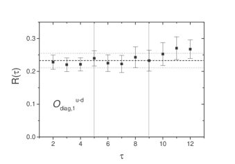
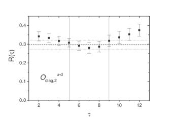
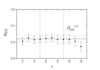
Figure 1: Plateau plots of the ratios $R(\tau,P^{\prime},P)$ for the $n=2$ operators ${\cal O}^{\text{u-d}}_{\text{diag,1}}$, ${\cal O}^{\text{u-d}}_{\text{diag,2}}$, and ${\cal O}^{\text{u-d}}_{\{20\}}$.

The resulting lattice matrix elements, together with their jackknife errors are as follows:

$$\overline{R}^{\text{u-d}}_{\text{diag,1}}(P^{\prime},P) = 0.2327\pm 0.0224\,,$$

$$\overline{R}^{\text{u-d}}_{\text{diag,2}}(P^{\prime},P) = 0.2970\pm 0.0235\,,$$

$$\overline{R}^{\text{u-d}}_{\text{diag,3}}(P^{\prime},P) = 0.00832\pm 0.01651\,,$$

$$\overline{R}^{\text{u-d}}_{\{10\}}(P^{\prime},P) = -0.09768\pm 0.01648\,,$$

$$\overline{R}^{\text{u-d}}_{\{20\}}(P^{\prime},P) = -0.1802\pm 0.0205\,,$$

$$\overline{R}^{\text{u-d}}_{\{21\}}(P^{\prime},P) = -0.05926\pm 0.01162\,.$$ (21)

We now consider a minimal set of three operators to determine, but not overdetermine, the three generalized form factors, $A^{\text{u-d}}_{20},B^{\text{u-d}}_{20}$, and $C^{\text{u-d}}_{20}$. The subset of diagonal operator equations alone are insufficient Schroers and QCDSF collaboration (2002), since the diagonal index combinations are linearly dependent and provide only a system of equations of rank two.

The minimal choice to determine, but not overdetermine, the form factors is to choose two diagonal operators and one off-diagonal operator, analogous to familiar procedures to calculate moments of parton distributionsGöckeler et al. (1996a); Dolgov et al. (2002) or electromagnetic form factors Göckeler et al. (2001); Göckeler et al. (2003a). The best choice for this purpose is the set of matrix elements $\langle P^{\prime}|{\cal O}^{\text{u-d}}_{\text{diag,1}}|P\rangle$, $\langle P^{\prime}|{\cal O}^{\text{u-d}}_{\text{diag,2}}|P\rangle$, and $\langle P^{\prime}|{\cal O}^{\text{u-d}}_{\{20\}}|P\rangle$, which have the smallest relative errors and provide a system of three linearly independent equations.

The form factors and associated errors determined this way are shown in Fig. 2 by the triangles plotted to at the left at $N=0$.

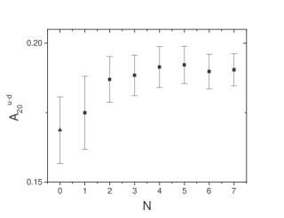
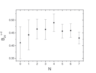
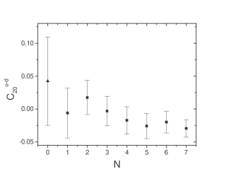
Figure 2: Generalized form factors obtained by simultaneous fits to $N$ external momentum combinations having virtuality $t_{\text{vlow}}$. As described in the text, the $N=0$ points, denoted by triangles, use three operators at a single external momentum combination to determine the three form factors. The remaining points, denoted by squares, use six operators and $N$ external momentum combinations to determine the three form factors.

Still considering the same single choice of external momenta, the full set of six matrix elements in Eq. (20) provides an overdetermined set of equations that yield the form factors and errors labeled $N=1$ in Fig 2. We previously argued that the $C$ form factor is least accurately determined because its coefficients have the highest powers of $\Delta$, and the minimally determined fit, $N=0$ bears out this expectation. Note that the overdetermined fit, $N=1$ leaves the errors in $A$ and $B$ roughly the same, but substantially reduces that of $C$. The results of the two fits agree within errors, but since the overdetermined fit exploits the maximal information in the lattice measurements, Eq. (III.1) and has smaller overall statistical errors, we consider it superior.

We now progress to the next level by including all the external momentum combinations enumerated in Tab. 1. The results are displayed in Fig. 2, where the abscissa denotes the total number of momentum combinations included in the fit. Entry $N$ corresponds to the inclusion of momentum sets $1,2,\cdots N$ of Tab. 1. As expected, the errors for each form factor decrease significantly as new statistical information is included by adding momenta in new directions. The improvement is generally less than $\sqrt{N}$ because measurements of different momenta on the same lattices are correlated.

The overall result in Fig. 2 is a strong validation of our approach. Comparing the minimally determined, $N=0$ result at the far left with the overdetermined result with all seven momentum combinations, $N=7$ at the far right, we observe that our method reduces the error in the least accurately determined form factor $C$ by a factor of 5, the error in $B$ by a factor of 3, and the error in $A$ by a factor of 2.

III.2 Generalized Form Factors and Quark Angular Momentum

Having validated our analysis technique, we now apply it to the full set of external momenta and virtualities listed in Appendix A, Tab. 2. The results of the full, overdetermined analysis for the flavor non-singlet generalized form factors $A^{\text{u-d}}_{20}(t)$, $B^{\text{u-d}}_{20}(t)$, and $C^{\text{u-d}}_{2}(t)$ are shown in Fig. 3. We observe that with the present analysis, all three generalized form factors are determined quite accurately throughout the full range of virtuality up to $t=3.1\,$GeV². As expected, some combinations of external momenta induce more statistical noise than others, but the overall structure of the form factors is well determined. Although there is no fundamental argument for the functional dependence on $t$, it is useful to fit the form factors to the dipole form that provides a good phenomenological fit to the nucleon electromagnetic form factors, and the results of least-squares fit by dipole form factors are shown for $A(t)$ and $B(t)$. Although the individual up and down form factors $C_{2}^{\text{u/d}}(t)$ are non-vanishing, their difference, $C_{2}^{\text{u-d}}(t)$, is statistically consistent with zero. We note this flavor independence is a feature of the Chiral Quark Soliton Model in Ref. Kivel et al. (2001).

Although results are not yet available at other quark masses to enable extrapolation to the physical quark mass, these results clearly show the behavior of the generalized form factors in the $900\,$MeV pion world. For this non-singlet case, there are no corrections from disconnected diagrams.

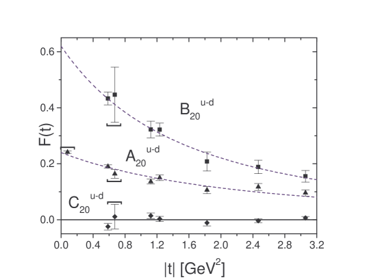
Figure 3: Generalized form factors $A^{\text{u-d}}_{20}(t)$, $B^{\text{u-d}}_{20}(t)$, and $C^{\text{u-d}}_{2}(t)$ for all available virtualities obtained using the full set of operators and external momentum combinations. The dashed curves denote dipole fits to $A$ and $B$ to guide the eye and extrapolate to $t=0$. The form factor $C$ is consistent with zero. Four data points, denoted by horizontal brackets, have been shifted by $|t|=0.2\,$GeV² to the right for clarity in plotting.

It is useful to point out that in all cases for which $t\neq 0$, there were no zero (or nearly zero) singular values in our calculations. Hence, in these cases, the singular value decomposition is completely equivalent to minimizing Eq. (18) by conventional least-squares analysis. In the case of $t=0$, because of the explicit factors of $\Delta$ appearing in Eq. (I), only the coefficients $A^{q}_{n0}(0)$ can be determined. As expected, the singular value decomposition handled this automatically, with the zero singular values resulting in minimization in the appropriate subspace of $A^{q}_{n0}(0)$. Note that this procedure introduces no bias or model assumptions. Rather, it simply specifies the correct physical subspace.

Since the total quark angular momentum is given by the zero virtuality limit, $J_{q}=\frac{1}{2}[A^{\text{u+d}}_{20}(0)+B^{\text{u+d}}_{20}(0)]$, it is particularly interesting to study this limit. Two issues need to be addressed. The first is extrapolation to $t=0$. This is not a problem for $A$, since it is just the moment of the spin-averaged parton distribution $A_{20}(0)=\langle x\rangle$. However, like the electromagnetic form factor $F_{2}$, $B$ cannot be measured at $t=0$ since the kinematical factors always contain $\Delta$, and therefore it must be extrapolated. From the behavior of the flavor non-singlet combination $B^{\text{u-d}}_{20}(t)$ in Fig. 3, one might expect significant extrapolation errors. However, as shown in Fig. 4, the cancellation between the up and down quark contributions is nearly complete and the flavor singlet combination $B^{\text{u+d}}_{20}(t)$ is consistent with zero. Hence, essentially the full contribution comes from $A^{\text{u+d}}_{20}(0)$.

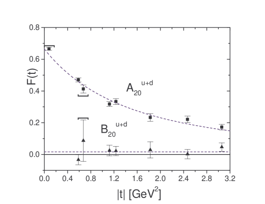
Figure 4: Flavor singlet generalized form factors $A^{\text{u+d}}_{20}(t)$ and $B^{\text{u+d}}_{20}(t)$ with dipole fits denoted by dashed curves. Note that the singlet combination $B^{\text{u+d}}_{20}(t)$ is consistent with zero, so that the total quark angular momentum $J_{q}=\frac{1}{2}[A^{\text{u+d}}_{20}(0)+B^{\text{u+d}}_{20}(0)]$ is dominated by $A$. Three data points, denoted by horizontal brackets, have been shifted by $|t|=0.2\,$GeV² to the right for clarity in plotting.

The second issue is the fact that disconnected diagrams, which are beyond the scope of the present work, must also be included in these flavor singlet matrix elements.

It is interesting to note that light cone arguments indicate that the contribution of each Fock space sector to the gravitomagnetic moment $B(0)=\sum_{q,g}B_{20}^{q,g}(0)=0$ is separately zero Brodsky et al. (2001). Although this may not necessarily imply that connected and disconnected diagrams for $B(0)$ separately cancel, it is suggestive of our result above that the connected contribution to $B(0)$ was consistent with zero. Note that the separate vanishing of quark and gluon contributions to $B(0)$ was also conjectured in Ref. Teryaev (1998).

With the caveat that we must omit disconnected diagrams for the present, we proceed to quote our lattice results from connected diagrams. Using the results of Ref. Dolgov et al. (2002) at $\kappa=0.1560$, the quark spin contribution to nucleon angular momentum is given by the lowest moment of the longitudinal spin distribution

$$\frac{1}{2}\Delta\Sigma = \frac{1}{2}[\langle 1\rangle_{\Delta u}+\langle 1\rangle_{\Delta d}]$$ (22)

$$\sim \frac{1}{2}\,\,0.682(18)\,.$$

Since $B^{\text{u+d}}_{20}(0)\sim 0$, the total quark spin and orbital contribution to the nucleon angular momentum is

$$J_{q} = \frac{1}{2}[A^{\text{u+d}}_{20}(0)+B^{\text{u+d}}_{20}(0)]$$ (23)

$$\sim \frac{1}{2}[\langle x\rangle_{u}+\langle x\rangle_{d}+0]$$

$$\sim \frac{1}{2}\,\,0.675(7)\,.$$

Thus, since these two results are equal within errors, if we consider only connected diagrams in the world of $900\,$MeV pions, we conclude that the quark spin produces 68 percent of the nucleon angular momentum and the quark orbital angular momentum contribution is negligible. Although this is superficially consistent with expectations from relativistic quark models, we note that serious physical interpretation and quantitative comparison with quark models requires consideration of the disconnected diagrams. The striking fact for our present purposes, however, is that it is possible to measure the connected part to the order of one percent, under the assumption that $B^{\text{u+d}}_{20}(0)=0\pm 0$.

Note that quenched connected diagram contributions of $\Delta\Sigma$ and $J_{q}$ have been reported in Refs. Mathur et al. (2000); Göckeler et al. (2003b). Since those calculations were performed for pion masses ranging above $500\,$MeV, we would expect quenching effects to be negligible and hence that their results would be statistically consistent with ours. The chiral extrapolated results of Göckeler et. al. Göckeler et al. (2003b) that 66 $\pm$ 14 percent of the nucleon spin arises from the quark spin and that 6 $\pm$ 14 percent arises from quark orbital angular momentum are completely compatible with our results because of the small quark mass dependence. The results for $\Delta\Sigma$ by Mathur et. al. in Ref. Mathur et al. (2000) are also consistent with ours. Reference Dolgov et al. (2002) showed that the linear extrapolation of $\Delta\Sigma$ is essentially constant, only changing from 68 $\pm$ 2 percent of the nucleon spin at $m_{\pi}=900\,$ MeV to 69 percent in the chiral limit. This is consistent with the connected diagram chiral extrapolation by Mathur et. al. of 62 $\pm$ 8 percent. The results for $J_{q}$, however, are inconsistent. From the results of their Fig. 3 and their 1.045 renormalization factor, $J_{q}$ contributes 84 $\pm$ 8 percent of the spin, which disagrees with our result of 68 $\pm$ 1 percent. We believe the discrepancy arises because Mathur et. al. use the dipole prescription to extrapolate the sum $A_{20}^{\text{u+d}}+B_{20}^{\text{u+d}}$, whereas, as shown in our Fig. 4, we calculate $A^{\text{u+d}}_{20}(0)$ directly without extrapolation and only extrapolate the nearly vanishing $B^{\text{u+d}}_{20}$.

IV Conclusions

In summary, we have presented a new method for calculating generalized form factors in lattice QCD that extracts the full information content from a given lattice configuration by measuring an overdetermined set of lattice observables. We demonstrated its effectiveness in an exploratory calculation of $n=2$ generalized form factors up to $3\,$GeV² and showed that it reduces errors to as small as one-fifth of those obtained by a conventional minimally-determined analysis. The final error bars for $A^{\text{u-d}}_{20}(t)$, $A^{\text{u+d}}_{20}(t)$, and $B^{\text{u-d}}_{20}(t)$ are typically of the order of five to ten percent, providing useful information about the Fourier transform of the transverse structure of the nucleon. Because of fortunate cancellation in the flavor singlet case, the connected diagram contributions to the total quark angular momentum are measured to the order of one percent. Although this exploratory calculation was performed for the heaviest of the three SESAM quark masses used in earlier calculation of moments of parton distributions, we expect the technique to be sufficiently robust to treat all the masses.

We note that the first calculation of generalized form factors were reported by Schroers in Schroers and QCDSF collaboration (2002) using the standard minimally-determined analysis, and more extensive calculations by the QCDSF collaboration using our method are being published simultaneously with this present work Göckeler et al. (2003b).

This work provides the foundation for a number of promising investigations. The $n=3$ relations introduced in this work enable us to calculate the $t$-dependence for three moments and thus explore the variation of the transverse structure of the proton with $x$. The same methodology can, of course, be used to calculate spin-dependent generalized form factors. In the longer term, extensive calculations with emerging multi-Teraflops computers dedicated to lattice QCD will enable the chiral and continuum calculations required to have definitive impact on the new generation of experiments currently being undertaken Airapetian et al. (2001); Stepanyan et al. (2001); Favart (2002).

Appendix A Matrix elements in terms of generalized form factors

In order to find the relation between Minkowski-expressions, e.g. $\left(\mathcal{O}^{\text{M}}\right)^{\{\mu_{1}\mu_{2}\dots\mu_{n}\}}$, and the corresponding Euclidean quantities, $\left(\mathcal{O}^{\text{E}}\right)_{\{\mu_{1}\mu_{2}\dots\mu_{n}\}}$, we observe that the operators under consideration are constructed from gamma matrices and covariant derivatives $D$. The conventions we use, consistent with Ref. Montvay and Münster (1994), are

$$\left(\gamma^{\text{E}}\right)_{\mu} = \sum_{\nu=1}^{4}h_{\mu\nu}\left(\gamma^{\text{M}}\right)^{\nu},\quad h_{\mu\nu}=\text{diag}\left(\text{i},\text{i},\text{i},1\right),$$

$$\left(D^{\text{E}}\right)_{\mu} = \sum_{\nu=1}^{4}d_{\mu\nu}\left(D^{\text{M}}\right)^{\nu},\quad d_{\mu\nu}=\text{diag}\left(1,1,1,-\text{i}\right)\,,$$

and we will set $\left(a^{\text{M}}\right)^{\nu=0}=$ $\left(a^{\text{M}}\right)^{\nu=4}$. Since all operators are symmetrized, the general transformation rule for the operators with one gamma matrix and $n-1$ covariant derivatives investigated in this work is given by

$$\left(\mathcal{O}^{\text{E}}\right)_{\{\mu_{1}\mu_{2}\dots\mu_{n}\}}=h_{\mu_{1}\nu_{1}}d_{\mu_{2}\nu_{2}}\dots d_{\mu_{n}\nu_{n}}\left(\mathcal{O}^{\text{M}}\right)^{\{\nu_{1}\nu_{2}\dots\nu_{n}\}},$$ (24)

where a summation over the indices $\nu_{i}$ is implicit. In the following, we will drop the label E or M, and it will be clear from the context if Euclidean or Minkowski expressions are used.

We write matrix elements in terms of Dirac spinors as follows

$$\left\langle P^{\prime}\right|\mathcal{O}\left|P\right\rangle=\overline{U}(P^{\prime}){\mathcal{K}}_{\mathcal{O}}(P^{\prime},P)U(P)\,.$$

The ratio $R_{\mathcal{O}}^{\text{cont}}(P^{\prime},P)$ can be written explicitly in Minkowski space as

$$\left.R_{\mathcal{O}}^{\text{cont}}(P^{\prime},P)\right|_{\text{ground state}} = \left(E(P^{\prime})E(P)\right)^{-1/2}$$ (25)

$$\quad\times\left(\frac{1}{2}\text{Tr}\left[\Gamma_{\text{unpol}}\left(\not{P}^{\prime}+m\right)\right]\frac{1}{2}\text{Tr}\left[\Gamma_{\text{unpol}}\left(\not{P}+m\right)\right]\right)^{-1/2}$$

$$\quad\times\frac{1}{4}\text{Tr}\left[\Gamma_{\text{pol}}\left(\not{P}^{\prime}+m\right)\mathcal{K}_{\mathcal{O}}(P^{\prime},P)\left(\not{P}+m\right)\right]\,,$$

neglecting all excited states which would introduce a time dependence. Note that $R_{\mathcal{O}}^{\text{cont}}(P^{\prime},P)$ is directly proportional to $\left\langle P^{\prime}\right|\mathcal{O}\left|P\right\rangle$. The ratio in Eq. (25) is expressed in a general form that applies to all quark bilinear operators and projectors $\Gamma_{\text{pol/unpol}}$ relevant to this work.

The Minkowski space expressions for the QCDSF and the LHPC projectors used in our analysis are as follows

$$\Gamma_{\text{unpol}}^{\text{LHPC}} = \frac{1}{4}\left(1+\gamma_{0}\right),\;\Gamma_{\text{pol}}^{\text{LHPC}}=\frac{1}{4}\left(1+\gamma_{0}\right)\left(1-\gamma_{5}\gamma_{3}\right)\,,$$ (26)

$$\Gamma_{\text{unpol}}^{\text{QCDSF}} = \frac{1}{2}\left(1+\gamma_{0}\right),\;\Gamma_{\text{pol}}^{\text{QCDSF}}=\frac{1}{2}\left(1+\gamma_{0}\right)\gamma_{5}\gamma_{2}\,.$$ (27)

We also record the complete expressions for the kernels $\mathcal{K}_{\mathcal{O}}(P^{\prime},P)$ in Eq. (25). Following the general parameterization of Ji (1997), we have for the lowest three moments $n=1,2,3$ in Minkowski space

$$\left\langle P^{\prime}\right|\mathcal{O}^{\{\mu_{1}\mu_{2}\dots\}}\left|P\right\rangle = \overline{U}(P^{\prime})\mathcal{K}_{\mathcal{O}}^{\{\mu_{1}\mu_{2}\dots\}}(P^{\prime},P)U(P)$$

$$\left\langle P^{\prime}\right|\overline{\psi}_{q}\gamma^{\mu_{1}}\psi_{q}\left|P\right\rangle = \overline{U}(P^{\prime})\left\{\gamma^{\mu_{1}}A_{q,1}(\Delta^{2})+\text{i}\frac{\sigma^{\mu_{1}\alpha}\Delta_{\alpha}}{2m}B_{q,1}(\Delta^{2})\right\}U(P)$$

$$\left\langle P^{\prime}\right|\overline{\psi}_{q}\gamma^{\{\mu_{1}}\overleftrightarrow{D}^{\mu_{2}\}}\psi_{q}\left|P\right\rangle = \overline{U}(P^{\prime})\left\{(-\text{i})\overline{P}^{\{\mu_{1}}\gamma^{\mu_{2}\}}A_{q,2}(\Delta^{2})\right.$$

$$+(-\text{i})\text{i}\overline{P}^{\{\mu_{1}}\frac{\sigma^{\mu_{2}\}\alpha}\Delta_{\alpha}}{2m}B_{q,2}(\Delta^{2})$$

$$+\left.(-\text{i})\frac{\Delta^{\{\mu_{1}}\Delta^{\mu_{2}\}}}{m}C_{q,2}(\Delta^{2})\right\}U(P)$$

$$\left\langle P^{\prime}\right|\overline{\psi}_{q}\gamma^{\{\mu_{1}}\overleftrightarrow{D}^{\mu_{2}}\overleftrightarrow{D}^{\mu_{3}\}}\psi_{q}\left|P\right\rangle = \overline{U}(P^{\prime})\left\{(-\text{i})^{2}\overline{P}^{\{\mu_{1}}\overline{P}^{\mu_{2}}\gamma^{\mu_{3}\}}A_{q,30}(\Delta^{2})\right.$$ (28)

$$+(-\text{i})^{2}\Delta^{\{\mu_{1}}\Delta^{\mu_{2}}\gamma^{\mu_{3}\}}A_{q,32}(\Delta^{2})$$

$$+\text{i}(-\text{i})^{2}\overline{P}^{\{\mu_{1}}\overline{P}^{\mu_{2}}\frac{\sigma^{\mu_{3}\}\alpha}\Delta_{\alpha}}{2m}B_{q,30}(\Delta^{2})$$

$$\left.+\text{i}(-\text{i})^{2}\Delta^{\{\mu_{1}}\Delta^{\mu_{2}}\frac{\sigma^{\mu_{3}\}\alpha}\Delta_{\alpha}}{2m}B_{q,32}(\Delta^{2})\right\}U(P)\,.$$

In practice, we evaluate the ratio $R_{\mathcal{O}}^{\text{cont,}\{\mu_{1}\mu_{2}\dots\}}(P^{\prime},P)$ by inserting the kernels $\mathcal{K}_{\mathcal{O}}^{\{\mu_{1}\mu_{2}\dots\}}$ from Eq. (28) and the projectors in Eq. (26,27) into Eq. (25). For given values of the nucleon momenta $P$ and $P^{\prime}$, the ratio is computed numerically, determining the kinematical coefficients of the GFFs $A(t)$, $B(t)$ and $C(t)$. Eventually, we transform the free indices $\{\mu_{1}\mu_{2}\dots\}$ to Euclidean space with the use of Eq. (24). The system of linear equations is then constructed by equating the Euclidean lattice result and the transformed Minkowskian parameterization.

A.1 Lattice operators

On the lattice side, we have H$\left(4\right)$-invariance instead of Lorentz-invariance, which complicates the classification and the renormalization of the operators. Following Göckeler et al. (1996b), we choose appropriate linear combinations of the operators $\mathcal{O}_{\{\mu_{1}\mu_{2}\dots\}}$, corresponding to representations of $H(4)$.

For the case of one derivative, $n=2$, there are three diagonal operators

$$\mathcal{O}_{1}^{\text{diag,n=2}} = \frac{1}{2}\left[\mathcal{O}_{11}+\mathcal{O}_{22}-\mathcal{O}_{33}-\mathcal{O}_{44}\right]\,,$$

$$\mathcal{O}_{2}^{\text{diag,n=2}} = \frac{1}{2^{1/2}}\left[\mathcal{O}_{33}-\mathcal{O}_{44}\right],$$

$$\mathcal{O}_{3}^{\text{diag,n=2}} = \frac{1}{2^{1/2}}\left[\mathcal{O}_{11}-\mathcal{O}_{22}\right]\,,$$ (29)

which are symmetric and traceless by construction. Additionally there are six non-diagonal combinations

$$\mathcal{O}_{\mu_{1},\mu_{2}}^{\text{non-diag,n=2}}=\frac{1}{2}\left[\mathcal{O}_{\mu_{1}\mu_{2}}+\mathcal{O}_{\mu_{2}\mu_{1}}\right]=\mathcal{O}_{\left\{\mu_{1}\mu_{2}\right\}},\quad\mu_{1,2}=1\dots 4;\;\mu_{1}<\mu_{2}\,,$$ (30)

giving in the most general case a set of nine independent operators. There is no operator mixing for $n=2$.

In the case of two derivatives, $n=3$, we take

$$\mathcal{O}_{1}^{\text{n=3}} = \left(\frac{3}{2}\right)^{1/2}\left[\mathcal{O}_{\left\{122\right\}}-\mathcal{O}_{\left\{133\right\}}\right],\quad\mathcal{O}_{2}^{\text{n=3}}=\frac{1}{2^{1/2}}\left[\mathcal{O}_{\left\{122\right\}}+\mathcal{O}_{\left\{133\right\}}-2\mathcal{O}_{\left\{144\right\}}\right],$$

$$\mathcal{O}_{3}^{\text{n=3}} = \left(\frac{3}{2}\right)^{1/2}\left[\mathcal{O}_{\left\{211\right\}}-\mathcal{O}_{\left\{233\right\}}\right],\quad\mathcal{O}_{4}^{\text{n=3}}=\frac{1}{2^{1/2}}\left[\mathcal{O}_{\left\{211\right\}}+\mathcal{O}_{\left\{233\right\}}-2\mathcal{O}_{\left\{244\right\}}\right],$$

$$\mathcal{O}_{5}^{\text{n=3}} = \left(\frac{3}{2}\right)^{1/2}\left[\mathcal{O}_{\left\{311\right\}}-\mathcal{O}_{\left\{322\right\}}\right],\quad\mathcal{O}_{6}^{\text{n=3}}=\frac{1}{2^{1/2}}\left[\mathcal{O}_{\left\{311\right\}}+O_{\left\{322\right\}}-2\mathcal{O}_{\left\{344\right\}}\right],$$

$$\mathcal{O}_{7}^{\text{n=3}} = \left(\frac{3}{2}\right)^{1/2}\left[\mathcal{O}_{\left\{411\right\}}-\mathcal{O}_{\left\{422\right\}}\right],\quad\mathcal{O}_{8}^{\text{n=3}}=\frac{1}{2^{1/2}}\left[\mathcal{O}_{\left\{411\right\}}+\mathcal{O}_{\left\{422\right\}}-2\mathcal{O}_{\left\{433\right\}}\right]\,,$$ (31)

while the four non-diagonal combinations are denoted by

$$\mathcal{O}_{\mu_{1},\mu_{2},\mu_{3}}^{\text{non-diag,n=3}}=\mathcal{O}_{\left\{\mu_{1}\mu_{2}\mu_{3}\right\}},\quad\mu_{1,2,3}=1\dots 4;\;\mu_{1}<\mu_{2}<\mu_{3}\,,$$

giving all in all 12 traceless and symmetric linear combinations. It turns out that some of the operators in Eqns. (31) mix with different non-symmetric representations (cf. Ref. Göckeler et al. (1996b)) under renormalization. Fortunately, the mixing coefficient turns out to be negligible, at least for the specific case considered in Göckeler et al. (1996a). It has to be checked if this holds true for all potential mixing candidates in the $n=3$ case.

The choice of index combinations for the construction of the H(4) operators is not unique. However, in the continuum limit all options will lead to the same GFFs. The interesting question of determining an optimal set of operators that minimizes lattice artifacts is beyond the scope of this presentation.

A.2 Lattice momenta

The possible values of the nucleon momenta $P$ and $P^{\prime}$ and therefore the momentum transfer squared $t$ are severely restricted by the lattice momenta. The general three-momentum on a periodic lattice is given by

$$\overrightarrow{P}=\frac{2\pi}{aL_{s}}\overrightarrow{p}=\frac{2\pi}{aL_{s}}\left(p_{1},p_{2},p_{3}\right),\quad p_{i}=-L_{s},-L_{s}+1,\dots,L_{s}-1,L_{s}\,,$$

where $a$ is the lattice spacing in GeV^-1 (we set $a=1$ in all intermediate steps), and $L_{s}$ is the spatial lattice extension, which is in our case $16$. It is clear that the lattice spacing times the spatial extension determines the smallest possible non-zero momentum, while the lattice spacing alone fixes the largest available momentum. In practice, however, we are even more restricted to values $p_{i}\ll L_{s}$, because large momenta lead to considerable noise. For the nucleon four momenta $P$ and $P^{\prime}$, we use the continuum dispersion relation, $P_{0}=P_{4}=\sqrt{m^{2}+\overrightarrow{P}^{2}}$, where $m$ is the nucleon mass, determined in our lattice calculation. In order to construct the maximally determined set of linear equations, Eq. (II.2), we need to know all $\overrightarrow{p},\overrightarrow{p}^{\prime}$ leading to the same momentum transfer squared $t$. So far we have propagators available for the two sink momenta $\overrightarrow{p}^{\prime}=\left(0,0,0\right)$ and $\overrightarrow{p}^{\prime}=\left(-1,0,0\right)$, and the value for $\overrightarrow{q}\equiv\overrightarrow{p}^{\prime}-\overrightarrow{p}$ is restricted by $\overrightarrow{q}^{2}<6$. We plan to extend the allowed values in future investigations. The total number of different $t$ is then 16, including the forward case.

Note, that $t$ depends in a nontrivial manner on $\overrightarrow{p}^{\prime}$ and $\overrightarrow{p}$ individually through the energies $P_{4},P_{4}^{\prime}$, and not only on the relative momentum $\overrightarrow{q}$. For 8 of the 16 possible values of $t$, we encountered highly visible fluctuations in the nucleon propagators with negative values for the two point functions at large $\tau\gg\tau_{\text{src}}$. We excluded the corresponding momentum combinations from our analysis. A list of all remaining $\overrightarrow{q},\overrightarrow{p}^{\prime},\overrightarrow{p}$ and $t$, is shown in table 2.

Table 2: Lattice momenta used in our calculation.

$\overrightarrow{p}^{\prime}$	$\overrightarrow{q}$	$\overrightarrow{p}$	$t$ [GeV2]
$\begin{array}[]{l}\left(0,0,0\right)\\ \left(-1,0,0\right)\end{array}$	$\begin{array}[]{l}\left(0,0,0\right)\\ \left(0,0,0\right)\end{array}$	$\begin{array}[]{l}\left(0,0,0\right)\\ \left(-1,0,0\right)\end{array}$	0
$\begin{array}[]{l}\left(0,0,0\right)\\ \left(-1,0,0\right)\end{array}$	$\begin{array}[]{l}\left(\pm 1,0,0\right),\left(0,\pm 1,0\right),\left(0,0,\pm 1\right)\\ \left(-1,0,0\right)\end{array}$	$\begin{array}[]{l}\left(\mp 1,0,0\right),\left(0,\mp 1,0\right),\left(0,0,\mp 1\right)\\ \left(0,0,0\right)\end{array}$	-0.592
$\left(-1,0,0\right)$	$\left(0,\pm 1,0\right),\left(0,0,\pm 1\right)$	$\left(-1,\mp 1,0\right),\left(-1,0,\mp 1\right)$	-0.597
$\left(0,0,0\right)$	$\left(\pm 1,\pm 1,0\right),\left(\pm 1,0,\pm 1\right),\left(0,\pm 1,\pm 1\right)$	$\left(\mp 1,\mp 1,0\right),\left(\mp 1,0,\mp 1\right),\left(0,\mp 1,\mp 1\right)$	-1.134
$\left(-1,0,0\right)$	$\left(-1,\pm 1,0\right),\left(-1,0,\pm 1\right)$	$\left(0,\mp 1,0\right),\left(0,0,\mp 1\right)$	-1.246
$\left(-1,0,0\right)$	$\left(-1,\pm 1,\pm 1\right)$	$\left(0,\mp 1,\mp 1\right)$	-1.844
$\left(-1,0,0\right)$	$\left(-2,0,0\right)$	$\left(1,0,0\right)$	-2.492
$\left(-1,0,0\right)$	$\left(-2,\pm 1,0\right),\left(-2,0,\pm 1\right)$	$\left(1,\mp 1,0\right),\left(1,0,\mp 1\right)$	-3.090

References

- Müller et al. (1994) D. Müller, D. Robaschik, B. Geyer, F. M. Dittes, and J. Horejsi, Fortschr. Phys. 42, 101 (1994), eprint hep-ph/9812448.
- Ji (1997) X.-D. Ji, Phys. Rev. Lett. 78, 610 (1997), eprint hep-ph/9603249.
- Radyushkin (1997) A. V. Radyushkin, Phys. Rev. D56, 5524 (1997), eprint hep-ph/9704207.
- Burkardt (2000) M. Burkardt, Phys. Rev. D62, 071503 (2000), eprint hep-ph/0005108.
- Ralston and Pire (2002) J. P. Ralston and B. Pire, Phys. Rev. D66, 111501 (2002), eprint hep-ph/0110075.
- Diehl (2002) M. Diehl, Eur. Phys. J. C25, 223 (2002), eprint hep-ph/0205208.
- Lai et al. (1997) H. L. Lai et al., Phys. Rev. D55, 1280 (1997), eprint hep-ph/9606399.
- Glück et al. (1998) M. Glück, E. Reya, and A. Vogt, Eur. Phys. J. C5, 461 (1998), eprint hep-ph/9806404.
- Martin et al. (2002) A. D. Martin, R. G. Roberts, W. J. Stirling, and R. S. Thorne, Eur. Phys. J. C23, 73 (2002), eprint hep-ph/0110215.
- Göckeler et al. (1996a) M. Göckeler et al., Phys. Rev. D53, 2317 (1996a), eprint hep-lat/9508004.
- Best et al. (1997) C. Best et al. (1997), eprint hep-ph/9706502.
- Göckeler et al. (1997) M. Göckeler et al., Nucl. Phys. Proc. Suppl. 53, 81 (1997), eprint hep-lat/9608046.
- Göckeler et al. (2001) M. Göckeler, R. Horsley, D. Pleiter, P. E. L. Rakow, and G. Schierholz (2001), eprint hep-ph/0108105.
- Dolgov et al. (2002) D. Dolgov et al. (LHPC), Phys. Rev. D66, 034506 (2002), eprint hep-lat/0201021.
- Detmold et al. (2001) W. Detmold, W. Melnitchouk, J. W. Negele, D. B. Renner, and A. W. Thomas, Phys. Rev. Lett. 87, 172001 (2001), eprint hep-lat/0103006.
- Belitsky et al. (2002) A. V. Belitsky, D. Müller, and A. Kirchner, Nucl. Phys. B629, 323 (2002), eprint hep-ph/0112108.
- Teukolsky et al. (1992) S. A. Teukolsky, W. T. Vetterling, and B. P. Flannery, Numerical Recipes in C (Cambridge University Press, 1992), 2nd ed.
- Schroers (2001) W. Schroers, Dissertation, Fachbereich Physik, Bergische Universität-Gesamthochschule Wuppertal (2001), eprint hep-lat/0304016.
- Schroers and QCDSF collaboration (2002) W. Schroers and QCDSF collaboration (2002), presented at the Workshop on “Hadronic phenomenology from lattice gauge theory” at the University of Regensburg, August 1-3, 2002.
- Göckeler et al. (2003a) M. Göckeler et al. (QCDSF) (2003a), eprint hep-lat/0303019.
- Kivel et al. (2001) N. Kivel, M. V. Polyakov, and M. Vanderhaeghen, Phys. Rev. D63, 114014 (2001), eprint hep-ph/0012136.
- Brodsky et al. (2001) S. J. Brodsky, D. S. Hwang, B.-Q. Ma, and I. Schmidt, Nucl. Phys. B593, 311 (2001), eprint hep-th/0003082.
- Teryaev (1998) O. V. Teryaev (1998), eprint hep-ph/9803403.
- Mathur et al. (2000) N. Mathur, S. J. Dong, K. F. Liu, L. Mankiewicz, and N. C. Mukhopadhyay, Phys. Rev. D62, 114504 (2000), eprint hep-ph/9912289.
- Göckeler et al. (2003b) M. Göckeler, R. Horsley, D. Pleiter, P. E. Rakow, A. Schäfer, G. Schierholz, and W. Schroers (2003b), eprint hep-ph/0304249.
- Airapetian et al. (2001) A. Airapetian et al. (HERMES), Phys. Rev. Lett. 87, 182001 (2001), eprint hep-ex/0106068.
- Stepanyan et al. (2001) S. Stepanyan et al. (CLAS), Phys. Rev. Lett. 87, 182002 (2001), eprint hep-ex/0107043.
- Favart (2002) L. Favart, Nucl. Phys. A711, 165 (2002), eprint hep-ex/0207030.
- Montvay and Münster (1994) I. Montvay and G. Münster, Quantum Fields on a Lattice, Cambridge Monographs on Mathematical Physics (Cambridge University Press, 1994).
- Göckeler et al. (1996b) M. Göckeler et al., Phys. Rev. D54, 5705 (1996b), eprint hep-lat/9602029.